Influence of the contacts on the conductance of interacting quantum wires

Abstract

We investigate how the conductance $G$ through a clean interacting quantum wire is affected by the presence of contacts and noninteracting leads. The contacts are defined by a vanishing two-particle interaction to the left and a finite repulsive interaction to the right or vice versa. No additional single-particle scattering terms (impurities) are added. We first use bosonization and the local Luttinger liquid picture and show that within this approach $G$ is determined by the properties of the leads regardless of the details of the spatial variation of the Luttinger liquid parameters. This generalizes earlier results obtained for step-like variations. In particular, no single-particle backscattering is generated at the contacts. We then study a microscopic model applying the functional renormalization group and show that the spatial variation of the interaction produces single-particle backscattering, which in turn leads to a reduced conductance. We investigate how the smoothness of the contacts affects $G$ and show that for decreasing energy scale its deviation from the unitary limit follows a power law with the same exponent as obtained for a system with a weak single-particle impurity placed in the contact region of the interacting wire and the leads.

I Introduction

The low-energy physics of one-dimensional (1d) metals is not described by the Fermi liquid theory if two-particle interactions are taken into account. Such systems fall into the Luttinger liquid (LL) universality classKS that is characterized by power-law scaling of a variety of correlation functions and a vanishing quasi-particle weight. For spin-rotational invariant interactions and spinless models, on which we focus here, the exponents of the different correlation functions can be parametrized by a single number, the interaction dependent LL parameter $K<1$ (for repulsive interactions; $K=1$ in the noninteracting case). As a second independent LL parameter one can take the velocity $v_{c}$ of charge excitations (for details see below). Instead of being quasi-particles the low lying excitations of LLs are collective density excitations. This implies that impurities or more generally inhomogeneities have a dramatic effect on the physical properties of LLs.LutherPeschel ; Mattis ; ApelRice ; Giamarchi

In the presence of only a single impurity on asymptotically small energy scales observables behave as if the 1d system was cut in two halfs at the position of the impurity, with open boundary conditions at the end points (open chain fixed point).KaneFisher ; Furusaki0 ; Fendley In particular, for a weak impurity and decreasing energy scale $s$ the deviation of the linear conductance $G$ from the impurity-free value scales as $(s/s_{0})^{2(K-1)}$, with $K$ being the scaling dimension of the perfect chain fixed point and $s_{0}$ a characteristic energy scale (e.g. the band width). This holds as long as $\left|V_{\rm back}/s_{0}\right|^{2}(s/s_{0})^{2(K-1)}\ll 1$, with $V_{\rm back}$ being a measure for the strength of the $2k_{F}$ backscattering of the impurity and $k_{F}$ the Fermi momentum. For smaller energy scales or larger bare impurity backscattering this behavior crosses over to another power-law scaling $G(s)\sim(s/s_{0})^{2(1/K-1)}$, with the scaling dimension of the open chain fixed point $1/K$. This scenario was verified for infinite LLsKaneFisher ; Furusaki0 ; Fendley as well as finite LLs connected to Fermi liquid leads,FurusakiNagaosa ; Tilman a setup that is closer to systems that can be realized in experiments. In the latter case the scaling holds as long as the contacts are modeled to be “perfect”, that is free of any bare and effective single-particle backscattering, and the impurity is placed in the bulk of the interacting quantum wire. For an impurity placed close to perfect contacts the exponents change to $2(K-1)/(K+1)$ (close to the perfect chain fixed point) and $1/K-1$ (close to the open chain fixed point).FurusakiNagaosa ; Tilman

The role of an inhomogeneous two-particle interaction, that is an interaction that depends not only on the relative distance of the two particles, but also the center of mass is less well understood. In the present publication we will fill this gap. Such an inhomogeneity will generically appear close to the interface of the interacting quantum wire and the leads and a detailed understanding is thus essential for the interpretation of transport experiments on quasi-1d quantum wires.experiments We here use two models to study the effect of two-particle inhomogeneities on the linear conductance. We first investigate the so-called local Luttinger liquid (LLL) model,SS ; MS ; Ponomarenko that is characterized by a spatial dependence of the LL parameters $K$ and $v_{c}$, with $K=1$ and $v_{c}=v_{F}$ in the leads ($v_{F}$ is the noninteracting Fermi velocity). We show that regardless of the details of the spatial variation the conductance always takes the perfect value $1/(2\pi)$ (in units such that $\hbar=1$ and the electron charge $e=1$). Thus the LLL description cannot produce any effective single-particle backscattering from the contact region generated by an inhomogeneous two-particle interaction. Our results generalize earlier findings obtained for step-like variations of the LL parameters.SS ; MS ; Ponomarenko

We then study a microscopic lattice model with a spatially dependent nearest-neighbor interaction. Across the contact between the left lead and the wire the interaction is turned on from zero to a bulk value $U$ and correspondingly turned off close to the right contact. We show that this two-particle inhomogeneity generically leads to an effective single-particle backscattering and a reduced conductance. To compute the latter we use an approximation scheme that is based on the functional renormalization group (fRG).Tilman We numerically and analytically investigate the dependence of the conductance on $U$, the length of the interacting wire $N$, and the “smoothness” with which the interaction is turned on and off. For weak effective inhomogeneities we analytically show that $1/(2\pi)-G$ displays scaling with the energy scale $\delta_{N}=\pi v_{F}/N$ set by the length of the wire. The exponent we find is consistent with the one found for a weak single-particle impurity close to a perfect contact.FurusakiNagaosa ; Tilman We give the energy scale up to which this scaling holds. It depends on the bulk interaction $U$ and the $2k_{F}$ Fourier component of the function with which the interaction is varied close to the contacts. The latter provides a quantitative measure of the “smoothness” of the contacts. This finding suggests a similarity between the universal low-energy properties of a LL with a single-particle inhomogeneity and a two-particle inhomogeneity. We discuss this similarity but also point out differences.

This paper is organized as follows. In Sec. II we study the two-particle inhomogeneity within the LLL picture. To motivate the LLL model in Sec. II.1 we present a brief introduction into bosonization and the Tomonaga-Luttinger model. The transport properties of the LLL model are investigated in Sec. II.2. In Sec. III we introduce our microscopic model and give the basic equations of the fRG approach. We then discuss our numerical results in Sec. III.1 and the analytical findings in Sec. III.2. We close in Sec. IV with a summary.

II The local Luttinger liquid description

In this section we discuss how sufficiently smooth contacts (perfect contacts) can be properly described in a LLL picture. This approach was successfully used to show that for perfect contacts the properties of the leads and not the finite size quantum wire determine the conductance.SS ; MS ; Ponomarenko Up to now the LL parameters were always assumed to vary step-like. Here we present a simple derivation of this result for an arbitrary variation of the LL parameters. Also the role of impurities in the interacting wire was investigated within the LLL picture.Maslov2 ; FurusakiNagaosa It was shown that the exponent of the temperature dependence of the conductance is different for impurities placed in the bulk and close to the contacts.FurusakiNagaosa Using the fRG this was later confirmed in a microscopic model in which the contacts were modeled to be arbitrarily smooth.Tilman .

II.1 Model and generalized wave equations

In order to also elucidate the limitations of the LLL picture we first shortly recall the basic ideas necessary to justify the Tomonaga-Luttinger-modelT ; L ; KS for interacting fermions in one dimension in the homogeneous case. We consider a system of length $L$ with periodic boundary conditions. In second quantization the two-body interaction reads

$$V = \frac{1}{2}\int\int v(x-x^{\prime})\delta\rho(x)\delta\rho(x^{\prime})dxdx^{\prime}$$ (1)

$$+\frac{1}{2L}{\cal N}^{2}\tilde{v}(0)-\frac{1}{2}v(0){\cal N},$$

where $\delta\rho(x)=\psi^{\dagger}(x)\psi(x)-{\cal N}/L$ is the operator of the particle density relative to its homogeneous value, with ${\cal N}$ the particle number operator. The Fourier transform of the two-body interaction is denoted as $\tilde{v}(k)$. The last term is usually dropped as it only modifies the chemical potential. If the range of the two-body interaction is much larger than the mean particle distance only particle-hole pairs in the vicinity of the two Fermi points are present in the ground state and the eigenstates with low excitation energy.T This allows to linearize the dispersion around the two Fermi points and to introduce two independent types of fermions, the right- and left-movers with particle density operators $\delta\rho_{\pm}(x)=\rho_{\pm}(x)-{\cal N_{\pm}}$

$$\delta\rho_{\alpha}(x) = \frac{1}{L}\sum_{n\neq 0}e^{ik_{n}x}\rho_{n,\alpha}=\frac{\partial}{\partial x}\left[\frac{-i}{2\pi}\sum_{n\neq 0}\frac{e^{ik_{n}x}}{n}\rho_{n,\alpha}\right]$$ (2)

$$\equiv \frac{\partial\Phi_{\alpha}}{\partial x}~{}.$$

As shown below the field operators $\Phi_{\alpha}$ are convenient objects for the solution of the problem.comment In the subspace of low energy states the Fourier components of the density $\rho_{n,\alpha}$ obey the commutation relationsT

$$[\rho_{m,\alpha},\rho_{n,\beta}]=\alpha m\,\delta_{\alpha\beta}\;\delta_{m,-n}~{}.$$ (3)

After proper normalization they take the form of boson commutation relations.

One can write the operator of the kinetic energy as a quadratic form of the $\rho_{\pm}$.T The Tomonaga model then results from replacing $\delta\rho(x)$ by $\delta\rho_{+}(x)+\delta\rho_{-}(x)$ and ${\cal N}$ by ${\cal N}_{+}+{\cal N}_{-}$ in Eq. (1). With the well known “g-ology” generalizationKS the boson part of the interaction reads

$$V_{\text{TL},b}=\frac{1}{2}\int\!\!\int\left\{2g_{2}(x-x^{\prime})\delta\rho_{+}(x)\delta\rho_{-}(x^{\prime})\right.$$ (4)

$$\left.+g_{4}(x-x^{\prime})\left[\delta\rho_{+}(x)\delta\rho_{+}(x^{\prime})+\delta\rho_{-}(x)\delta\rho_{-}(x^{\prime})\right]\right\}dxdx^{\prime}\;.$$

This reduces to Tomonaga’s original model for $g_{2}\equiv g_{4}\equiv v$, while LuttingerL later independently studied the model with $g_{4}\equiv 0$. He also discussed the special case $g_{2}(x)\sim\delta(x)$, which corresponds to the interaction term in the massless Thirring model.TM This simplifies various aspects but brings in infinities which have to be removed e.g. by normal ordering. In the boson part of the kinetic energy

$$T_{b}=\pi v_{F}\int\left[\delta\rho_{+}^{2}(x)+\delta\rho_{-}^{2}(x)\right]dx$$ (5)

the integrand has to be normal ordered. This, as above, is usually suppressed.

Inhomogeneous Luttinger liquids can be realized by adding an external one-particle potential or by allowing the two-body interaction to depend on both spatial variables, i.e. $v(x-x^{\prime})$ in Eq. (1) is replaced by $v(x,x^{\prime})$. The operator of a one-particle potential can only be expressed in terms of the $\delta\rho_{\alpha}$ if it is sufficiently smooth in real space, i.e. the external potential has a vanishing $2k_{F}$ Fourier component. Similarly only for sufficiently smooth variations—in Sec. III.2 we will specify the meaning of “sufficiently smooth”—of $v$ with $(x+x^{\prime})/2$ the analogous steps from Eq. (1) to Eq. (4) i.e. $g_{i}(x-x^{\prime})\to g_{i}(x,x^{\prime})$ are allowed without changing the low energy physics. The standard LLL model is obtained by assuming $g_{i}(x,x^{\prime})=g_{i,x}\delta(x-x^{\prime})$

$$H_{\text{LLL},b} = \pi\int\left\{\left(v_{F}+\frac{g_{4,x}}{2\pi}\right)\left[\delta\rho_{+}^{2}(x)+\delta\rho_{-}^{2}(x)\right]+\frac{g_{2,x}}{\pi}\delta\rho_{+}(x)\delta\rho_{-}(x)\right\}dx$$ (6)

$$= \frac{\pi}{2}\int\left\{\left(v_{F}+\frac{g_{4,x}+g_{2,x}}{2\pi}\right)\left[\frac{\partial\Phi^{(+)}(x)}{\partial x}\right]^{2}+\left(v_{F}+\frac{g_{4,x}-g_{2,x}}{2\pi}\right)\left[\frac{\partial\Phi^{(-)}(x)}{\partial x}\right]^{2}\right\}dx$$

$$\equiv \frac{\pi}{2}\int\left\{v_{N}(x)\left[\frac{\partial\Phi^{(+)}(x)}{\partial x}\right]^{2}+v_{J}(x)\left[\frac{\partial\Phi^{(-)}(x)}{\partial x}\right]^{2}\right\}dx~{},$$

where we have defined $\Phi^{(\pm)}(x)\equiv\Phi_{+}(x)\pm\Phi_{-}(x)$, as well as the velocities $v_{N}(x)$ and $v_{J}(x)$. As in the homogeneous model the right and left movers are coupled by the $g_{2}$ interaction and using the $\Phi^{(\pm)}(x)$ as the basic fields simplifies the solution as $\Phi^{(\nu)}(x)$ and $\Phi^{(\nu)}(x^{\prime})$ commute. Apart from a term which vanishes in the thermodynamic limit $\Phi^{(-\nu)}(x^{\prime})$ and $\partial\Phi^{(\nu)}(x)/\partial x$ obey canonical commutation relations after proper normalization

$$\left[\frac{\partial\Phi^{(\nu)}(x)}{\partial x},\Phi^{(-\nu)}(x^{\prime})\right]=\frac{i}{\pi}\left[\delta_{L}(x-x^{\prime})-\frac{1}{L}\right]\;.$$ (8)

This follows from Eqs. (2) and (3). Here $\delta_{L}$ denotes the $L$-periodic delta function. Neglecting the correction term yields the following Heisenberg equations of motion for the $\Phi^{(\nu)}(x,t)$

$$\frac{\partial}{\partial t}\Phi^{(+)}(x,t) = -v_{J}(x)\frac{\partial\Phi^{(-)}(x,t)}{\partial x}\;,$$

$$\frac{\partial}{\partial t}\Phi^{(-)}(x,t) = -v_{N}(x)\frac{\partial\Phi^{(+)}(x,t)}{\partial x}\;.$$ (9)

Therefore, the $\Phi^{(\nu)}(x,t)$ obey generalized wave equations, e.g. for the field related to the change of the total density

$$\frac{\partial^{2}}{\partial t^{2}}\Phi^{(+)}(x,t)-v_{J}(x)\frac{\partial}{\partial x}v_{N}(x)\frac{\partial\Phi^{(+)}(x)}{\partial x}=0\;.$$ (10)

The spatial derivative of the first equation in Eq. (II.1) yields the continuity equation for the total charge density $\delta\rho=\delta\rho_{+}+\delta\rho_{-}$

$$\frac{\partial}{\partial t}\delta\rho(x,t)+\frac{\partial}{\partial x}\left[v_{J}(x)\frac{\partial\Phi^{(-)}(x,t)}{\partial x}\right]=0$$ (11)

which implies the conservation of the total charge $Q=\int\delta\rho dx$. As Eqs. (10) and (11) are linear the expectation values discussed in the following obey the same equations.

In a homogeneous system the velocities $v_{J}$ and $v_{N}$ are constant and the corresponding “sound velocity” called the charge velocity $v_{c}$ is given by $v_{c}=\sqrt{v_{J}v_{N}}$. It constitutes the first LL parameter characterizing the system. The second LL parameter $K$ is defined as $K\equiv\sqrt{v_{J}/v_{N}}=v_{c}/v_{N}$. The general solution of the wave equation for constant $v_{c}$ and $K$ reads $f(x-v_{c}t)+g(x+v_{c}t)$, where $f$ and $g$ are arbitrary functions.

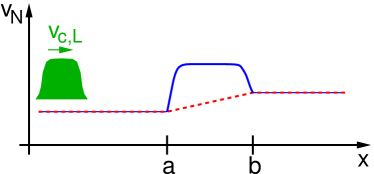
Figure 1: (Color online) Spatial dependence of velocity $v_{N}(x)$ used for the discussion of the generalized wave equation (10). Two different realizations (full and dashed curves) of the transition region $[a,b]$ are shown. The shaded area shows the incoming density $\delta\rho(x,0)$.

II.2 Computing the transmitted charge

For general dependencies of $v_{J}(x)$ and $v_{N}(x)$ on the position the generalized wave equation (10) cannot be solved analytically. In the following we discuss properties of the solution in the thermodynamic limit when the velocities $v_{J}(x)$ and $v_{N}(x)$ are constant for $x<a$ and $x>b>a$ but have arbitrary (bounded) variation in the interval $[a,b]$. Figure 1 shows two qualitatively different types of behavior of $v_{N}(x)$. The dashed curve presents a monotonous transition between the asymptotic values while the full curve corresponds to an “interacting wire” region in $[a,b]$ with a higher (constant) value of $v_{N,w}$ corresponding to a stronger repulsive interaction. In order to describe the charge transport through this region we consider an incoming density with compact support which at $t=0$ is completely to the left of $a$ and moves towards it with constant velocity $v_{c,L}$ (see Fig. 1). Before the disturbance reaches point $a$ the time evolution is

$$\Phi^{(+)}(x,t)=f_{\rm in}(x-v_{c,L}t)\;,\;\;\;\delta\rho(x,t)=f_{\rm in}^{\prime}(x-v_{c,L}t)\;.$$ (12)

The total incoming charge $Q_{\rm in}$ is given by $Q_{\rm in}=f_{\rm in}(a)-f_{\rm in}(-\infty)$. This short time solution for $\Phi^{(+)}(x,t)$ determines $\Phi^{(-)}(x,t)$ up to a constant. In the long time limit there will again be no charge in the region $[a,b]$ with the total transmitted charge $Q_{\rm trans}$ moving to the right with constant velocity $v_{c,R}$ and the total reflected charge $Q_{\rm ref}$ moving to the left with velocity $v_{c,L}$, where charge conservation implies $Q_{\rm trans}+Q_{\rm ref}=Q_{\rm in}$. In the following we show that it is possible to determine $Q_{\rm ref}/Q_{\rm in}$ without the explicit solution for $\delta\rho(x,t)$ in this long time limit and without any additional assumptions on the spatial variation of $v_{N}(x)$ and $v_{J}(x)$. The trick is to introduce the quantity

$$S(t) \equiv \int_{-\infty}^{\infty}\frac{1}{v_{J}(x)}\frac{\partial\Phi^{(+)}(x,t)}{\partial t}dx$$

$$= \Phi^{(-)}(-\infty,t)-\Phi^{(-)}(\infty,t)$$

and to show that $S$ is time independent. This can be seen by discussing the expression in the second line which follows using Eq. (II.1) or if one wants to argue with the density only by taking the time derivative and using the generalized wave equation

$$\dot{S}(t) = \int_{-\infty}^{\infty}\frac{1}{v_{J}(x)}\frac{\partial^{2}\Phi^{(+)}(x,t)}{\partial t^{2}}dx$$

$$= \int_{-\infty}^{\infty}\frac{\partial}{\partial x}\left[v_{N}(x)\frac{\partial}{\partial x}\Phi^{(+)}(x)\right]dx$$

$$= v_{N,R}\delta\rho(\infty,t)-v_{N,L}\delta\rho(-\infty,t)=0\;,$$

where we have used that the assumption about the initial state implies that $\rho(\pm\infty,t)$ vanishes for all finite times. The constant value of $S$ follows from Eq. (12)

$$S = -\int_{-\infty}^{a}\frac{v_{c,L}}{v_{J,L}}f_{\rm in}^{\prime}(x-v_{c,L}t)dx$$ (15)

$$= -\frac{v_{c,L}}{v_{J,L}}Q_{\rm in}=-\frac{Q_{\rm in}}{K_{L}}\;.$$

When the incoming density hits the transition region $[a,b]$ it is partially reflected and transmitted, where the detailed behavior is very different for the two realizations of $v_{N}(x)$ shown in Fig. 1. For sufficiently large times the total charge in the transition region goes to zero and $\Phi^{(+)}(x,t)$ takes the form

$$\Phi^{(+)}(x,t)=\left\{\begin{array}[]{ll}f_{\rm ref}(x+v_{c,L}t)\;,&{\rm for}\;x<a\\ \mbox{ const.}\;,&{\rm for}\;a<x<b\\ f_{\rm trans}(x-v_{c,R}t)\;,&{\rm for}\;x>b\;.\\ \end{array}\right.$$ (19)

With the definition of $S$ in Eq. (II.2) this yields

$$S = \frac{v_{c,L}}{v_{J,L}}\int_{-\infty}^{a}f_{\rm ref}^{\prime}(x+v_{c,L}t)dx$$ (20)

$$-\frac{v_{c,R}}{v_{J,R}}\int_{b}^{\infty}f_{\rm trans}^{\prime}(x-v_{c,r}t)dx$$

$$= \frac{Q_{\rm ref}}{K_{L}}-\frac{Q_{\rm trans}}{K_{R}}\;.$$

The comparison of Eqs. (15) and (20) as well as charge conservation leads to the result derived earlier assuming a stepwise variation of the LL parametersSS ; MS ; Ponomarenko

$$Q_{\rm ref}=\frac{K_{L}-K_{R}}{K_{L}+K_{R}}~{}Q_{\rm in}\;,\;\;\;Q_{\rm trans}=\frac{2K_{R}}{K_{L}+K_{R}}~{}Q_{\rm in}\;.$$ (21)

Our result shows that the properties of the transition region play no role at all. The ratio $Q_{\rm trans}/Q_{\rm in}$ is positive, while $Q_{\rm ref}/Q_{\rm in}$ has no definite sign.

From this result one can easily obtain the linear conductance $G$ through the system. We first discuss a homogeneous system with constant LL parameters $K_{L}$ and $v_{c,L}$ (the use of the index $L$ becomes clear later). We consider a current free initial state in which the density is increased by $\delta\rho_{0}$ in the left half of the infinite system. Then half of the additional density moves to the right with velocity $v_{c,L}$ which corresponds to the current

$$j=\frac{1}{2}v_{c,L}\delta\rho_{0}=\frac{1}{2}v_{c,L}\frac{\partial\rho}{\partial\mu}~{}\delta\mu_{0}\equiv G~{}\delta\mu_{0}$$ (22)

in the central region extending linearly with time. Here $\mu$ denotes the chemical potential. With $\partial\rho/\partial\mu=1/(\pi v_{N})$ this yields for the homogeneous system

$$G_{\rm hom}=\frac{K_{L}}{2\pi}\;.$$ (23)

We now switch to an inhomogeneous system as in Fig. 1. In analogy to the initial condition in the homogeneous case we raise the density for $x<a$ by $\delta\rho_{0}$. The stationary current is then obtained by multiplying the result for the homogeneous case by the fraction of transmitted charge through $[a,b]$, computed in Eq. (21). For the conductance this leads to

$$G_{\rm inhom}=\frac{2K_{R}K_{L}}{K_{L}+K_{R}}~{}\frac{1}{2\pi}\;,$$ (24)

which again is independent of the details of the transition region.

For an interacting quantum wire in region $[a,b]$ attached to noninteracting leads ($K_{L}=K_{R}=1$) the conductance is $1/(2\pi)$ independently of how quickly the LL parameters vary spatially near the contact points $a$ and $b$. This shows that the LLL description cannot produce one-particle backscattering from the contact region generated by an inhomogeneous two-particle interaction. As we will discuss next using a microscopic model and the fRG approach contacts defined by a vanishing interaction to the left and a positive finite interaction to the right (or vice versa) generically produce an effective single-particle backscattering. This clearly shows the limitations of the LLL picture. With the approximation to describe the two-body interaction as a quadratic form in the bose-fields the dependence of the conductance on the sharpness of the transition is lost. In contrast, our microscopic model directly allows to study the transition from smooth to abrupt contacts with the concomitant change of the conductance.

III A microscopic model

As our microscopic model we consider the spinless tight-binding Hamiltonian with nearest-neighbor hopping $\tau>0$ and a spatially dependent nearest-neighbor interaction $U_{j,j+1}=U_{j+1,j}$

$$H = -\tau\sum_{j=-\infty}^{\infty}\left(\,c^{{\dagger}}_{j+1}c_{j}^{\phantom{{\dagger}}}+c^{{\dagger}}_{j}\,c_{j+1}^{\phantom{{\dagger}}}\,\right)$$ (25)

$$+\sum_{j=1}^{N-1}U_{j,j+1}\left(n_{j}-1/2\right)\left(n_{j+1}-1/2\right)\;,$$

where we used standard second-quantized notation with $c^{{\dagger}}_{j}$ and $c_{j}^{\phantom{{\dagger}}}$ being creation and annihilation operators on site $j$, respectively, and $n_{j}=c^{{\dagger}}_{j}\,c_{j}^{\phantom{{\dagger}}}$ the local density operator. The interaction acts only between the bonds of the sites $1$ to $N$, which define the interacting wire. We later take

$$U_{j,j+1}=Uh(j)\,,\;\;\;j=1,2,\ldots,N-1\;,$$ (26)

with a function $h$ that is different from 1 only in regions close to the contacts at sites 1 and $N$. We here mainly consider the half-filled band case $n=1/2$. In the interacting region the fermions have higher energy compared to the leads. To avoid that the interacting wire is depleted (implying a vanishing conductance) we added a compensating single-particle term. It can be included as a shift of the local density operator by $1/2$. This ensures that the average filling in the leads and the wire is $n=1/2$. It is important to have a definite filling in the interacting wire as the LL parameters depend on $n$. For general fillings the required shift of the density depends on $n$ and the interaction.Tilman

The model Eq. (25) with nearest neighbor interaction $U$ across all bonds (not only the once within $1$ and $N$) is a LL for all $U$ and fillings, except at half filling for $|U|>2\tau$.Haldane At $n=1/2$ the LL parameter $K$ is given byHaldane

$$K=\left[\frac{2}{\pi}\,\arccos\left(-\frac{U}{2\tau}\right)\right]^{-1}\;,$$ (27)

for $|U|\leq 2\tau$. To leading order in $U/\tau$ this gives

$$K=1-\frac{U}{\pi\tau}+{\mathcal{O}}\left([U/\tau]^{2}\right)\;.$$ (28)

At temperature $T=0$ the linear conductance of the system described by Eq. (25) can be written asfootnote1

$$G(N)=\frac{1}{2\pi}\;|t(0,N)|^{2}$$ (29)

with the effective transmission $|t(\varepsilon,N)|^{2}=(4\tau^{2}-[\varepsilon+\mu]^{2})|{\mathcal{G}}_{1,N}(\varepsilon,N)|^{2}$. The one-particle Green function ${\mathcal{G}}$ has to be computed in the presence of interaction and in contrast to the noninteracting case acquires an $N$ dependence. To compute ${\mathcal{G}}$ and thus $G$ we use a recently developed fRG scheme.VM1 The starting point is an exact hierarchy of differential flow equations for the self-energy $\Sigma^{\Lambda}$ and higher order vertex functions, where $\Lambda\in(\infty,0]$ denotes an infrared energy cutoff which is the flow parameter. We here introduce $\Lambda$ as a cutoff for the Matsubara frequency. A detailed account of the method is given in Ref. Tilman, . We truncate the hierarchy by neglecting the flow of the two-particle vertex only considering $\Sigma^{\Lambda}$, which is then energy independent. The self-energy $\Sigma^{\Lambda=0}$ at the end of the fRG flow provides an approximation for the exact $\Sigma$. This approximation scheme and variants of it were successfully used to study a variety of transport problems through 1d wires of correlated electrons. In particular, in all cases of inhomogeneous LLs studied the exponents of power-law scaling were reproduced correctly to leading order in $U$.VM2 ; Tilman ; Xavier ; Xavier2

On the present level of approximation the fRG flow equation for the self-energy reads

$$\frac{\partial}{\partial\Lambda}\Sigma^{\Lambda}_{1^{\prime},1}=-\frac{1}{2\pi}\sum_{\omega=\pm\Lambda}\sum_{2,2^{\prime}}\,e^{i\omega 0^{+}}\,{\mathcal{G}}^{\Lambda}_{2,2^{\prime}}(i\omega)\,\Gamma_{1^{\prime},2^{\prime};1,2}\;,$$ (30)

where the lower indices $1$, $2$, etc. label single-particle states, $\Gamma_{1^{\prime},2^{\prime};1,2}$ is the bare antisymmetrized two-particle interaction and

$${\mathcal{G}}^{\Lambda}(i\omega)=\left[{\mathcal{G}}_{0}^{-1}(i\omega)-\Sigma^{\Lambda}\right]^{-1}\;,$$ (31)

with the noninteracting propagator ${\mathcal{G}}_{0}$. For the initial condition of the self-energy flow see below. As our single-particle basis we later use Wannier states [as in the Hamiltonian (25)] as well as momentum states.

III.1 Numerical results

In the real space Wannier basis the self-energy matrix is tridiagonal and the set of coupled differential equations (30) reads (with $j\in[1,N]$)

$$\frac{d}{d\Lambda}\Sigma^{\Lambda}_{j,j}=-\frac{1}{2\pi}\sum_{l=\pm 1}\sum_{\omega=\pm\Lambda}U_{j,j+l}{\mathcal{G}}^{\Lambda}_{j+l,j+l}(i\omega)\,e^{i\omega 0^{+}}\;,$$ (32)

$$\frac{d}{d\Lambda}\Sigma^{\Lambda}_{j,j\pm 1}=\frac{U_{j,j\pm 1}}{2\pi}\sum_{\omega=\pm\Lambda}{\mathcal{G}}^{\Lambda}_{j,j\pm 1}(i\omega)\,e^{i\omega 0^{+}}\,.$$ (33)

To derive these equations we have used that

$$\Gamma_{j^{\prime}_{1},j^{\prime}_{2};j_{1},j_{2}}=\bar{U}_{j_{1},j_{2}}\,(\delta_{j_{1},j^{\prime}_{1}}\delta_{j_{2},j^{\prime}_{2}}-\delta_{j_{1},j^{\prime}_{2}}\delta_{j_{2},j^{\prime}_{1}})$$ (34)

with $\bar{U}_{j_{1},j_{2}}=U_{j_{1},j_{1}+1}(\delta_{j_{1},j_{2}-1}+\delta_{j_{1},j_{2}+1})$. The initial condition of $\Sigma^{\Lambda}$ at $\Lambda=\infty$ isVM1 ; Tilman

$$\Sigma^{\infty}_{j,j} = -\left(U_{j-1,j}+U_{j,j+1}\right)/2\;,$$

$$\Sigma^{\infty}_{j,j\pm 1} = 0\;.$$ (35)

Even for very large $N$ (earlier results were obtained for up to $N=10^{7}$)Tilman ; VM2 the system Eqs. (32) and (33) can easily be integrated numerically starting at a large but finite $\Lambda_{0}$. Due to the slow decay of the right-hand-side (rhs) of the flow equation the integration from $\infty$ to $\Lambda_{0}$ gives a nonvanishing contribution on the diagonal of the self-energy matrix that does not vanish even for $\Lambda_{0}\to\infty$ and that exactly cancels the term in Eq. (III.1) such that

$$\Sigma^{\Lambda_{0}}_{j,j} = 0\;,$$

$$\Sigma^{\Lambda_{0}}_{j,j\pm 1} = 0\;.$$ (36)

For half filling the Hamiltonian (25) is particle-hole symmetric. For $N$ odd and symmetric $h(j)$, that is $h(j)=h(N-1-j)$, on which we focus here, it is furthermore invariant under inversion at site $j=(N+1)/2$. Together these symmetries lead to a vanishing conductance as was discussed earlier.Oguri1 ; VM3 We thus only consider even $N$. The two extreme cases of (a) an abrupt turning on and off of the interaction $h(j)=1$ for $j=1,2,\ldots,N-1$, and zero otherwise, and (b) a very smooth variation of $h(j)$ were considered earlier. In case (a) $1/(2\pi)-G$ increases for fixed $N$ and increasingVM2 ; VM3 $U$ as well as for fixed $U$ and increasing $N$.VM2 Using our fRG scheme it was shown that for asymptotically large $N$, $G$ vanishes as

$$G\sim(\delta_{N}/\tau)^{2(1/K-1)}\;,$$ (37)

with the energy scale $\delta_{N}=\pi v_{F}/N$. The scale on which the asymptotic low-energy scaling sets in strongly depends on $U$ and even for up to $N=10^{6}$ it was only reached for fairly large $U$, e.g. $U=1.5\tau$. As discussed in the introduction scaling of $G$ with the same exponent as in Eq. (37) is found for a single impurity in an otherwise perfect chain. This suggests that the low-energy physics of a correlated quantum wire with two contact inhomogeneities due to the two-particle interaction is similar to that of a wire with a single impurity (single-particle term). Here we will further investigate this relation.

Already at this stage it is important to note that the similarity is not complete. As shown elsewhereSeverin $G(T)$ for two contacts, fixed $U$, fixed large $N$, and decreasing temperature $T$ vanishes as (for $T\gg\delta_{N}$)

$$G\sim(T/\tau)^{1/K-1}\;,$$ (38)

that is with an exponent that is only one-half of the one found in the $\delta_{N}$ scaling Eq. (37). This is in clear contrast to the temperature dependence of $G$ for a single impurity in an otherwise perfect chain. In this case the exponent $2(1/K-1)$ is found in the scaling with any infrared energy scale, e.g. $T$, $\delta_{N}$, and $\Lambda$.

For a given $N$ and $U$ it is always possible to find a sufficiently smooth function $h(j)$ such that $1/(2\pi)-G$ is smaller then an arbitrarily small upper bound [case (b)].Tilman ; VM2 In that case the contacts are perfect and the effect of impurities in the interacting wire connected to Fermi liquid leads can be studied. Further down we will give a quantitative definition of the meaning of “sufficiently smooth”.

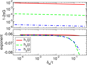
Figure 2: (Color online) Upper panel: The conductance $1-2\pi G$ as a function of $\delta_{N}/\tau$ for $U/\tau=0.2$, contacts of $m=7$ lattice sites, and three different contact functions $h_{i}(j)$ of increasing smoothness. Lower panel: The effective exponent (logarithmic derivative) of the data. The thin solid line shows the exponent $2(K-1)/(K+1)$ with $K(U/\tau=0.2)=0.9401$.

Here we study the dependence of the conductance on $N$, $U$, and the function $h(j)$ by numerically solving the flow equations (32) and (33) with the initial condition Eq. (III.1). In Fig. 2 we show $1-2\pi G$ as a function of $\delta_{N}/\tau\sim 1/N$ on a log-log scale (upper panel) for $U/\tau=0.2$ and three different $h(j)$ of increasing smoothness. In our numerical calculations for simplicity we focus on contact functions $h(j)$ that are symmetric around the middle of the interacting wire (equal contacts) and therefore only give their definition for the first half of the wire (with $j\in[1,N-1]$)

$$h_{1}(j) = 1\,,\;\;j=1,\ldots,N/2\;,$$

$$h_{2}(j) = \left\{\begin{array}[]{ll}j/m\,,&\;\;j=1,\ldots,m-1\\ 1\,,&\;\;j=m,\ldots,N/2\end{array}\right.\;,$$

and

$$h_{3}(j)=\left\{\begin{array}[]{ll}2(j/m)^{2}\,,&\;j=1,\ldots,(m-1)/2\\ 1-2(j/m-1)^{2}\,,&\;j=(m+1)/2,\ldots,m-1\\ 1\,,&\;j=m,\ldots,N/2\end{array}\right.,$$

where $m$ is odd and measures the length of the contact region. In Fig. 2 we chose $m=7$. The lower panel of Fig. 2 shows the logarithmic derivative of the data. A plateau in this figure corresponds to power-law scaling of the original data with an exponent given by the plateau value. For fixed $\delta_{N}$, $1-2\pi G$ decreases quickly with increasing smoothness of $h(j)$. For sufficiently small $\delta_{N}/\tau$ all curves follow power-law scaling. The smoother the contact the smaller $\delta_{N}/\tau$ has to be before the scaling sets in. The numerical exponent is close to $2(K-1)/(K+1)$ (shown as the thin solid line), with $K$ from Eq. (27). The latter is the exponent found for a system with perfect contacts and a weak single-particle impurity placed in the contact region. We also studied other values for the length of contact $m$ and found similar results. The deviation $1-2\pi G$ from the unitary limit decreases if $m$ is increased while all other parameters are fixed.

Within our approximation scheme we map the many-body problem on an effective single-particle problem with the energy independent $\Sigma^{\Lambda=0}$ as an impurity potential.VM1 ; Tilman During the fRG flow the interplay of the two-particle inhomogeneity and the bulk interaction generates an oscillating self-energy with an amplitude that decays slowly away from the two contacts. This is in close analogy to the case of a single impurity in an otherwise perfect chain.Glazman ; VM1 ; Tilman Scattering off this effective potential leads to the reduced conductance.

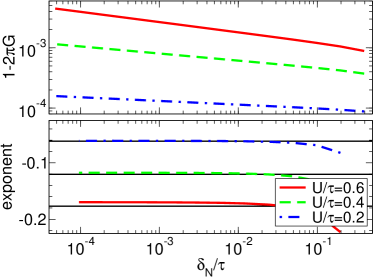
Figure 3: (Color online) Upper panel: The conductance $1-2\pi G$ as a function of $\delta_{N}/\tau$ for the contact function $h_{2}(j)$, contacts of $m=7$ lattice sites, and $U/\tau=0.2$, $0.4$, $0.6$. Lower panel: The effective exponent (logarithmic derivative) of the data. The thin solid lines show the exponents $2(K-1)/(K+1)$ with $K(U/\tau=0.2)=0.9401$, $K(U/\tau=0.4)=0.8864$, and $K(U/\tau=0.6)=0.8375$.

The $U$ dependence of $1-2\pi G$ and the effective exponent is shown in Fig. 3 for $h_{2}(j)$. At fixed $\delta_{N}$ the deviation of the conductance from the unitary limit increases with $U$. For all $U/\tau$ shown we find power-law behavior with exponents that are close to $2(K-1)/(K+1)$ (again shown as the thin solid lines). The larger $U/\tau$ the larger is the deviation of the numerical exponent and $2(K-1)/(K+1)$. This is not surprising as our approximate scheme can only be expected to capture exponents to leading order in $U/\tau$.Tilman

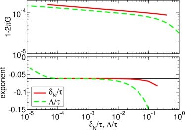
Figure 4: (Color online) Upper panel: The conductance $1-2\pi G$ as a function of $\delta_{N}/\tau$ and $\Lambda/\tau$ (with $N=2^{16}$ sites) for the contact function $h_{2}(j)$, contacts of $m=7$ lattice sites, and $U/\tau=0.2$. Lower panel: The effective exponent (logarithmic derivative) of the data. The thin solid line shows the exponents $2(K-1)/(K+1)$ with $K(U/\tau=0.2)=0.9401$.

For later reference we note that power-law behavior is not only found in the $\delta_{N}$ (that is $1/N$) dependence of $1-2\pi G$ but also in the dependence on the fRG flow parameter $\Lambda$ at a large fixed $N$. In this case $G$ is computed using Eq. (29) with the Green function at scale $\Lambda$. This is shown in Fig. 4 where we compare the dependence on $\delta_{N}/\tau$ and $\Lambda/\tau$ for $U=0.2$ and $h_{2}(j)$. Scaling with $\Lambda/\tau$ holds roughly down to the scale $\delta_{N}/\tau=\pi v_{F}/(\tau N)$ set by the length of the interacting wire. Beyond this scale $G$ saturates.

We now analytically confirm the power-law scaling of $1/(2\pi)-G$ for weak effective inhomogeneities and compute the exponent to leading order in the bulk interaction.

III.2 Analytical results

Numerically we found that $1/(2\pi)-G$ shows power-law scaling in both effective low-energy cutoffs $\delta_{N}$ and $\Lambda$, as long as the scaling variable considered is sufficiently larger than the other fixed energy scale. We note that the same holds for the temperature $T$ as the variable.Sabineprivate In all cases the same exponent is found. Analytically the easiest access to scaling is by considering $N\to\infty$, $T=0$, and taking $\Lambda$ as the variable. We will here follow this route. For the case of a single impurity with bare backscattering amplitude $V_{\rm back}$ in an infinite LL (no Fermi liquid leads) a similar calculation was performed within the fRGVM1 to show that for small $\Lambda$

$$\Sigma_{k_{F},-k_{F}}/\tau\sim(V_{\rm back}/\tau)\;(\Lambda/\tau)^{-U/(\pi\tau)}\;.$$ (41)

Within the Born approximation this leads to

$$\frac{K}{2\pi}-G\sim\left|V_{\rm back}/\tau\right|^{2}(\Lambda/\tau)^{-2U/(\pi\tau)}\;,$$ (42)

where $-2U/(\pi\tau)$ is the leading order approximation of the weak impurity exponent $2(K-1)$ [see Eq. (28)]. This scaling holds as long as the rhs stays small. For analytical calculations it is advantageous to switch from the real space basis to the momentum states.

In the momentum state basis the flow equation (30) is given by

$$\frac{\partial}{\partial\Lambda}\Sigma^{\Lambda}_{k^{\prime},k}=-\frac{1}{2\pi}\sum_{\omega=\pm\Lambda}\int_{-\pi}^{\pi}dq\,dq^{\prime}\,e^{i\omega 0^{+}}\,{\mathcal{G}}^{\Lambda}_{q,q^{\prime}}(i\omega)\,\Gamma_{k^{\prime},q^{\prime};k,q}\;,$$ (43)

with

$$\Gamma_{k^{\prime},q^{\prime};k,q} = \frac{1}{2\pi}\left[e^{i(q-q^{\prime})}-e^{i(q-k^{\prime})}+e^{i(k-k^{\prime})}-e^{i(k-q^{\prime})}\right]$$ (44)

$$\times\tilde{U}(k+q-k^{\prime}-q^{\prime})$$

and the Fourier transform of the interaction

$$\tilde{U}(k) = \frac{1}{2\pi}\sum_{j=1}^{N-1}U_{j+1,j}e^{ijk}$$ (45)

$$= U\;\tilde{h}(k)\;.$$

Here $\tilde{h}(k)$ denotes the Fourier transform of the function $h(j)$ that contains the shape of the turning on and off of the interaction. In the present section we do not assume special symmetry properties of $h(j)$. Thus the two contacts might be different, as it is generically the case in experiments. At $\Lambda=\Lambda_{0}$ all matrix elements of $\Sigma^{\Lambda_{0}}$ are zero. We now expand the rhs of Eq. (43) to first order in $\Sigma^{\Lambda}$. This expansion is justified as long as $\Sigma^{\Lambda}$ remains small (it is certainly small at the beginning of the fRG flow). The flow equation then becomes an inhomogeneous, linear differential equation

$$\frac{\partial}{\partial\Lambda}\Sigma^{\Lambda}_{k^{\prime},k}={\mathcal{F}}^{(1)}_{k^{\prime},k}(\Lambda)+{\mathcal{F}}^{(2)}_{k^{\prime},k}\left(\Lambda,\Sigma^{\Lambda}\right)\;,$$ (46)

with

$${\mathcal{F}}^{(1)}_{k^{\prime},k}(\Lambda)=-\frac{1}{2\pi}\sum_{\omega=\pm\Lambda}\int_{-\pi}^{\pi}dq\,\frac{\Gamma_{k^{\prime},q;k,q}}{i\omega-\xi_{q}}$$

$$=-\frac{U}{2\pi\tau}\tilde{h}(k-k^{\prime})\left(e^{ik}+e^{-ik^{\prime}}\right)\left(1-\frac{\Lambda}{\sqrt{\Lambda^{2}+4\tau^{2}}}\right)\,,$$ (47)

where we used $\xi_{k}=-2\tau\cos{(k)}-\mu$ and Eq. (44). The factor $e^{i\omega 0^{+}}$ was dropped as the integration starts at $\Lambda_{0}<\infty$. Later we will primarily be interested in the $k_{F},-k_{F}$ matrix element (backscattering) of $\Sigma$. For these momenta the rhs simplifies to

$${\mathcal{F}}^{(1)}_{k_{F},-k_{F}}(\Lambda)=-\frac{U}{\pi\tau}\tilde{h}(-2k_{F})e^{-ik_{F}}\left(1-\frac{\Lambda}{\sqrt{\Lambda^{2}+4\tau^{2}}}\right)\;.$$ (48)

The term on the rhs of the linearized flow equation that contains $\Sigma^{\Lambda}$ is

$${\mathcal{F}}^{(2)}_{k^{\prime},k}(\Lambda,\Sigma^{\Lambda}) = -\frac{1}{2\pi}\sum_{\omega=\pm\Lambda}\int_{-\pi}^{\pi}dq\,dq^{\prime}\,\Gamma_{k^{\prime},q^{\prime};k,q}$$ (49)

$$\times\left({\mathcal{G}}_{0}\Sigma^{\Lambda}{\mathcal{G}}_{0}\right)_{q,q^{\prime}}\;.$$

Before further evaluating this term we take $N\to\infty$ and compute $\Gamma_{k^{\prime},q;k,q}$ in this limit. As we will see in this case the information about the smoothness of $h(j)$ is lost on the rhs of Eq. (49). It nevertheless enters the solution of the differential equation via the inhomogeneity ${\mathcal{F}}^{(1)}_{k^{\prime},k}$ in Eq. (46). As we are only interested in the leading divergent behavior of the linear part on the rhs of Eq. (46) this procedure is justified. To be specific we first assume that the interaction is turned on and off abruptly, that is $h(j)=1$ for $j=1,2,\ldots,N-1$ and zero otherwise. To obtain the Fourier transform of the two-particle interaction we have to perform

$$\tilde{U}(k) = U\tilde{h}(k)=\frac{U}{2\pi}\sum_{j=1}^{N-1}e^{ijk}$$ (50)

$$= \frac{U}{2\pi}\frac{e^{ik}-e^{iNk}}{1-e^{ik}}$$

$$\stackrel{{\scriptstyle N\to\infty}}{{\longrightarrow}} U\,\frac{1}{2}\,\delta_{2\pi}(k)\;.$$

With this result the two-particle vertex simplifies to

$$\Gamma_{k^{\prime},q;k,q} \stackrel{{\scriptstyle N\to\infty}}{{\longrightarrow}} \frac{U}{\pi}\;\left[\cos(k-k^{\prime})-\cos(q-k^{\prime})\right]$$ (51)

$$\times\delta_{2\pi}(k+q-k^{\prime}-q^{\prime})\;.$$

Up to a factor $1/2$ the vertex is then equivalent to the one obtained for a homogeneous nearest neighbor interaction. With this vertex ${\mathcal{F}}^{(2)}_{k^{\prime},k}(\Lambda,\Sigma^{\Lambda})$ Eq. (49) reads

$${\mathcal{F}}^{(2)}_{k^{\prime},k}(\Lambda,\Sigma^{\Lambda})=-\frac{U}{2\pi^{2}}\sum_{\omega=\pm\Lambda}\int_{-\pi}^{\pi}dq[\cos(k-k^{\prime})$$

$$-\cos(q-k^{\prime})]\frac{\Sigma_{q+k-k^{\prime},q}}{(i\omega-\xi_{q+k-k^{\prime}})(i\omega-\xi_{q})}\;.$$ (52)

The differential equation (46) can be solved by the variation of constant method. To apply this we first determine the solution of the homogeneous equation. The scaling can be extracted if only the leading singular contribution (for $\Lambda\to 0$) of ${\mathcal{F}}^{(2)}_{k^{\prime},k}(\Lambda,\Sigma^{\Lambda})$ Eq. (52) at $k^{\prime}=k_{F}$ and $k=-k_{F}$ is kept. Following the same steps as in Ref. VM1, we find

$$\frac{\partial}{\partial\Lambda}\left[\Sigma^{\Lambda}_{k_{F},-k_{F}}\right]_{\rm hom}\approx-\frac{U}{2\pi\tau}\;\frac{1}{\Lambda}\left[\Sigma^{\Lambda}_{k_{F},-k_{F}}\right]_{\rm hom}\;,$$ (53)

with the solution

$$\left[\Sigma^{\Lambda}_{k_{F},-k_{F}}\right]_{\rm hom}/\tau\approx c_{0}\;(\Lambda/\tau)^{-U/(2\pi\tau)}\,,$$ (54)

where $c_{0}$ is a dimensionless constant. The singular part of the solution of the inhomogeneous linear differential equation is then given by

$$\Sigma^{\Lambda}_{k_{F},-k_{F}}/\tau\approx c(\Lambda)\;(\Lambda/\tau)^{-U/(2\pi\tau)}\,,$$ (55)

with

$$c(\Lambda)=\int_{\Lambda_{0}}^{\Lambda}d\Lambda^{\prime}\;\frac{1}{\left[\Sigma^{\Lambda^{\prime}}_{k_{F},-k_{F}}\right]_{\rm hom}}\;{\mathcal{F}}^{(1)}_{k_{F},-k_{F}}(\Lambda^{\prime})\;.$$ (56)

For small $\Lambda$ the function $c(\Lambda)$ is non-singular and given by

$$\lim_{\Lambda\to 0}c(\Lambda)=-\frac{U}{\tau}\tilde{h}(-2k_{F})e^{-ik_{F}}\;\bar{c}$$ (57)

with $\bar{c}$ being a constant of order $1$. This gives

$$\Sigma^{\Lambda}_{k_{F},-k_{F}}/\tau\approx-\frac{U}{\tau}\tilde{h}(-2k_{F})e^{-ik_{F}}\;\bar{c}\;(\Lambda/\tau)^{-U/(2\pi\tau)}$$ (58)

and with the Born approximation the final result

$$\frac{1}{2\pi}-G\sim\left|U/\tau\right|^{2}\;\left|\tilde{h}(-2k_{F})\right|^{2}\;(\Lambda/\tau)^{-U/(\pi\tau)}\;.$$ (59)

To obtain the singular part of the solution of the homogeneous differential equation $\left[\Sigma^{\Lambda}_{k_{F},-k_{F}}\right]_{\rm hom}$ we assumed that the interaction is turned on and off abruptly. One can show that the parts of $h(j)$ with a smooth variation of finite length do not contribute to the singular part of Eq. (49). Thus the same singular part is found independently of how the interaction is varied and Eq. (59) is valid for general $h(j)$.

The power-law scaling Eq. (59) holds for $\Lambda_{c}\ll\Lambda\ll\tau$ with a scale $\Lambda_{c}$ set by

$$\left|U/\tau\right|^{2}\;\left|\tilde{h}(-2k_{F})\right|^{2}\;(\Lambda_{c}/\tau)^{-U/(\pi\tau)}\sim 1/(4\pi)\;.$$ (60)

To leading order in $U/\tau$ the exponent $U/(\pi\tau)$ agrees with the exponent $2(K-1)/(K+1)$ [see Eq. (28)] found for a single weak impurity placed close to a perfect (that is arbitrarily smooth) contact.FurusakiNagaosa ; Tilman We thus have analytically shown, that with respect to the scaling exponent weak single-particle and weak two-particle inhomogeneities are indeed equivalent. The leading order exponent is furthermore consistent with the numerical results of the last section.

For the single impurity case the prefactor of the power law is given by $\left|V_{\rm back}/\tau\right|^{2}$. In case of the two-particle inhomogeneity this is replaced by the square of the bulk interaction and the square of the $2k_{F}$ Fourier component (backscattering) of the function $h(j)$ with which the interaction is turned on and off. The smaller this component the smaller is the perturbation due to the two contacts. Therefore the smoothness of the turning on and off is directly measured by $\tilde{h}(-2k_{F})$. The presence of the factor $|U/\tau|^{2}$ explains why in the numerical study the weak inhomogeneity exponent for larger $U/\tau$ is only observable for fairly smooth contacts, that is $h(j)$’s with small $2k_{F}$ component. For larger $U/\tau$ and fairly abrupt contacts the rhs of Eq. (59) becomes too large already on intermediate energy scales and no energy window for scaling is left. For $\Lambda\ll\Lambda_{c}$ defined in Eq. (60) the inhomogeneity is effectively large and Eq. (37) holds.

We here considered the half-filled band case, but also other fillings can be studied following the same steps.VM1

The analysis Eqs. (43) to (59) also holds if in addition weak single-particle impurities are placed close to the contacts, with the only difference that $\Sigma^{\Lambda_{0}}_{k_{F},-k_{F}}$ now has a non-vanishing initial condition set by the backscattering of the bare impurity. The prefactor in Eq. (59) is determined by either the square of the single impurity backscattering amplitude or $\left|U/\tau\right|^{2}\;\left|h(-2k_{F})\right|^{2}$ depending on the relative size.

IV Summary

In the present paper we have investigated the role of contacts, defined by an inhomogeneous two-particle interaction, on the linear conductance through an interacting 1d quantum wire. The wire and contacts were assumed to be free of any bare single-particle impurities. We first showed that within the LLL picture the contacts are always perfect, that is the conductance is $1/(2\pi)$ independent of the strength of the interaction, the length of the wire, and the spatial variation of the LL parameters. Earlier only step-wise changes of the LL parameters were considered. We then studied the problem within a microscopic lattice model. Similar to the case of a single impurity the interplay of the two-particle inhomogeneity and the bulk interaction generates an oscillating self-energy with an amplitude that decays slowly away from the contacts. Scattering off this effective potential leads to the discussed effects. We showed that within the microscopic modeling $1/(2\pi)-G$ increases with increasing bulk interaction $U$, increasing wire length $N$, and decreasing smoothness. The measure for smoothness is given by $\tilde{h}(-2k_{F})$, that is the backscattering Fourier component of the spatial variation $h(j)$ of the two-particle interaction. As long as the inhomogeneity stays effectively small $1/(2\pi)-G$ shows power-law scaling with an exponent that is consistent with $2(K-1)/(K+1)$, the scaling exponent known for the case of a wire with a single impurity placed close to one of the two smooth contacts.

In experiments on quantum wires the leads are electronically two- or three-dimensional. Depending on the systems studied the contacts are either regions in which the system gradually crosses over from higher dimensions to quasi 1d or the contact regions extend over a finite part of the wire (see the experiments on carbon nanotubes).experiments This shows that our simplified description—1d leads, spatially dependent interactions close to end contacts, no explicit single-particle scattering at the contacts—provides only an additional step towards a detailed understanding of the role of contacts in transport through interacting quantum wires, such as carbon nanotubes and cleaved edge overgrowth samples.experiments

References

- (1) For a review see K. Schönhammer in Interacting Electrons in Low Dimensions, Ed.: D. Baeriswyl, Kluwer Academic Publishers (2005).
- (2) A. Luther and I. Peschel, Phys. Rev. B 9, 2911 (1974).
- (3) D.C. Mattis, J. Math. Phys. 15, 609 (1974).
- (4) W. Apel and T.M. Rice, Phys. Rev. B 26, 7063 (1982).
- (5) T. Giamarchi and H.J. Schulz, Phys. Rev. B 37, 325 (1988).
- (6) C.L. Kane and M.P.A. Fisher, Phys. Rev. Lett. 68, 1220 (1992); Phys. Rev. B 46, 15233 (1992).
- (7) A. Furusaki and N. Nagaosa, Phys. Rev. B 47, 4631 (1993).
- (8) P. Fendley, A.W.W. Ludwig, and H. Saleur, Phys. Rev. Lett. 74, 3005 (1995).
- (9) A. Furusaki and N. Nagaosa, Phys. Rev. B 54, R5239 (1996).
- (10) T. Enss, V. Meden, S. Andergassen, X. Barnabé-Thériault, W. Metzner, and K. Schönhammer, Phys. Rev. B 71, 155401 (2005).
- (11) M. Bockrath, D. Cobden, J. Lu, A. Rinzler, R. Smalley, L. Balents, and P. McEuen, Nature 397, 598 (1999); Z. Yao, H. Postma, L. Balents, and C. Dekker, Nature 402, 273 (1999); O. Auslaender, A. Yacoby, R. de Picciotto, K. Baldwin, L. Pfeiffer, and K. West, Phys. Rev. Lett. 84, 1764 (2000); R. de Picciotto, H. Stormer, L. Pfeiffer, K. Baldwin, and K. West, Nature 411, 51 (2001).
- (12) I. Safi and H.J. Schulz, Phys. Rev. B 52, R17040 (1995).
- (13) D.L. Maslov and M. Stone, Phys. Rev. B 52, R5539 (1995).
- (14) V.V. Ponomarenko, Phys. Rev. B 52, R8666 (1995).
- (15) D.L. Maslov, Phys. Rev. B 52, R14368 (1995).
- (16) S. Tomonaga, Progr. Theor. Phys. 5, 544 (1950).
- (17) J.M. Luttinger, J. Math. Phys. 4, 1154 (1963).
- (18) There is no generally accepted use of prefactors in the definition of the in the literature. We therefore did not include any.
- (19) W. Thirring, Ann. Phys. (NY) 3, 91 (1958).
- (20) F.D.M. Haldane, Phys. Rev. Lett. 45, 1358 (1980).
- (21) Under quite weak assumptions on the frequency dependence of the self-energy, that are fulfilled for the present situation, there are no current vertex corrections at and Eq. (29) is exact (Ref. Oguri2, ).
- (22) A. Oguri, J. Phys. Soc. Jpn. 70, 2666 (2001).
- (23) V. Meden, W. Metzner, U. Schollwöck, and K. Schönhammer, J. Low Temp. Phys. 126, 1147 (2002).
- (24) V. Meden, S. Andergassen, W. Metzner, U. Schollwöck, and K. Schönhammer, Europhys. Lett. 64, 769 (2003).
- (25) X. Barnabé-Thériault, A. Sedeki, V. Meden, and K. Schönhammer, Phys. Rev. Lett. 94, 136405 (2005).
- (26) X. Barnabé-Thériault, A. Sedeki, V. Meden, and K. Schönhammer, Phys. Rev. B 71, 205327 (2005).
- (27) A. Oguri, Phys. Rev. B 59, 12240 (1999); ibid. 63, 115305 (2001).
- (28) V. Meden and U. Schollwöck, Phys. Rev. B 67, 193303 (2003).
- (29) S. Jakobs, T. Enss, V. Meden, and H. Schoeller, in preparation.
- (30) D. Yue, L.I. Glazman, and K.A. Matveev, Phys. Rev. B 49, 1966 (1994).
- (31) S. Andergassen, private communication.