Properties of the reaction front in a reaction-subdiffusion process

Abstract

We study the reaction front for the process $A+B\to C$ in which the reagents move subdiffusively. We propose a fractional reaction-subdiffusion equation in which both the motion and the reaction terms are affected by the subdiffusive character of the process. Scaling solutions to these equations are presented and compared with those of a direct numerical integration of the equations. We find that for reactants whose mean square displacement varies sublinearly with time as $\langle r^{2}\rangle\sim t^{\gamma}$, the scaling behaviors of the reaction front can be recovered from those of the corresponding diffusive problem with the substitution $t\to t^{\gamma}$.

I Introduction

It is very well known that diffusion-limited binary reactions in low dimensions exhibit “anomalous” rate laws, that is, rate laws that deviate from the quadratic forms that usually characterize binary reactions. It is also known that these anomalies occur because diffusion is not an effective mixing mechanism, especially in constrained geometries, whereas the quadratic rate laws assume perfect mixing. The shortcomings of diffusion as a mixing process lead to the spontaneous occurrence of spatial order and spatial structures in terms of which the anomalous rate laws are well understood kotomin . Broadly speaking, spatial order leads to a slowing down of the reaction because it tends to decrease or deplete the interfacial areas where reactions can occur.

The anomalies exhibit themselves in different ways according to the design of the experiment, and the critical dimension above which the behavior of the reaction is “normal” also varies from one experiment to another. Thus, for example, in an irreversible batch reaction $A+B\to C$, the decay of reactant concentrations deviates from (is slower than) the mean field behavior $\rho\sim t^{-1}$ up to dimension $d=4$. This anomaly is accompanied by and directly associated with a sharp segregation of species as the majority species in any region eliminates the minority species and diffusion is too slow to replenish the minority population effectively. If there are random sources of reactants so that the system achieves a steady state, species segregation is observed in the steady state up to dimension $d=2$ kotomin ; we1 .

One of the more accessible experimental setups to observe these anomalies is that of a reaction front in which initially one reactant uniformly occupies all the space to one side of a sharp front, and the other reactant occupies the other galfi . As the reaction proceeds, one can monitor the concentration profiles of both reactants and of the product. Their evolution reflect the anomalies. For the reaction-diffusion case the front evolution has been extensively studied theoretically and confirmed experimentally we2 .

Our interest lies in understanding binary reaction kinetics in media where the reactants move subdiffusively. Subdiffusive motion is particularly important in the context of complex systems such as glassy and disordered materials, in which pathways are constrained for geometric or for energetic reasons. It is also particularly germane to the way in which experiments in low dimensions have to be carried out. Such experiments must avoid any active or convective or advective mixing so as to ensure that any mixing is only a consequence of diffusion. To accomplish this usually requires the use of gel substrates and/or highly constrained geometries (the first gel-free experiments were carried out recently gelfree ; baroud ). Under these circumstances it is not clear whether the motion of the species is actually diffusive, or if it is in fact subdiffusive. Indeed, a recent detailed discussion on ways to extract accurate parameters and exponents from such experiments concludes that at least the experiments presented in that work, carried out in a gel, reflect subdiffusive rather than diffusive motion recent .

Subdiffusive motion is characterized by a mean square displacement that varies sublinearly with time,

$$\langle r^{2}(t)\rangle\sim\frac{2K_{\gamma}}{\Gamma(1+\gamma)}t^{\gamma},$$ (1)

with $0<\gamma<1$. For ordinary diffusion $\gamma=1$, and $K_{1}\equiv D$ is the ordinary diffusion coefficient. Subdiffusion is not modeled in a universal way in the literature. Among the more successful approaches to the subdiffusion problem have been continuous time random walks with non-Poissonian waiting time distributions Kehr ; Bouchaud ; Barkai ; Sokolov , and fractional dynamics approaches in which the ordinary diffusion operator is replaced by a generalized fractional diffusion operator Barkai ; Metzler ; West ; Hilfer ; Sch . The relation between the two has also been discussed. In particular, the fractional dynamics formulation that leads to the mean square displacement (1) can be associated with a continuous time random walk with a waiting time distribution between steps which at long times behaves as

$$\psi(t)\sim t^{-\gamma-1}.$$ (2)

In our work we adopt the fractional dynamics approach.

Since subdiffusion is an even poorer mixing mechanism than ordinary diffusion, we expect that the diffusive anomalies observed in constrained geometries will in some sense be exacerbated in a subdiffusive environment. However, the outcome is not entirely clear or predictable. On the one hand, slower motion naturally leads to a slowing down of the reaction. On the other, slower motion also delays the elimination of the minority species in a region, and therefore may reduce the spatial segregation effects observed in the diffusive case.

In this paper we focus on the time dependence of the front geometry, and, in particular, on the exponents that describe the evolution of a number of quantities that define the reaction front. We expect there to be anomalies that differ from those of the diffusive problem. In Sec. II we formulate our model and present our scaling solutions. In Sec. III we compare our scaling results with those obtained by direct numerical integration of our model equations. We end with some comments on our results in Sec. IV

II Evolution of subdiffusive front

We start with a system of $A$ particles on one side and $B$ particles on the other of a sharp linear front, defined to lie perpendicular to the $x$ axis. The particles diffuse and react with a given probability upon encounter. A standard mean-field model for the evolution of the concentrations $a(x,t)$ and $b(x,t)$ of $A$ and $B$ particles along $x$ is given by the reaction-diffusion equations

$$\begin{array}[]{rcl}\displaystyle\frac{\partial}{\partial t}a(x,t)&=&D\displaystyle\frac{\partial^{2}}{\partial x^{2}}a(x,t)-ka(x,t)b(x,t)\\ \vskip 3.0pt plus 1.0pt minus 1.0pt\cr\displaystyle\frac{\partial}{\partial t}b(x,t)&=&D\displaystyle\frac{\partial^{2}}{\partial x^{2}}b(x,t)-ka(x,t)b(x,t)\;,\end{array}$$ (3)

where $D$ is the diffusion coefficient assumed to be equal for the two species. The initial conditions are that $a(x,t)=const=a_{0}$ for $x<0$ and $a(x,t)=0$ for $x\geq 0$. Similarly, $b(x,t)=const=b_{0}$ for $x>0$ and $b(x,t)=0$ for $x\leq 0$. With these conditions, no matter the dimensionality of the system, the system of equations is effectively one-dimensional.

The front problem was first analyzed via a scaling description galfi and later refined by a large number of authors using more rigorous theoretical and careful numerical approaches (see references in Yuste et al. we2 ). One upshot of the extensive work is that $d=2$ is a critical dimension for the mean field description to be appropriate. Below $d=2$ one must take into account fluctuations, neglected in this description, that completely change the outcome of the analysis. While it has been assumed that the mean field model holds for the critical dimensions $d=2$, Krapivsky krapivsky finds logarithmic corrections that have also been observed in simulations cornell1 . Our program is to generalize the mean field description to the subdiffusive case and to apply a scaling description to the problem. One can show that $d=2$ is also the critical dimension for the subdiffusive problem. Our work is therefore not appropriate for systems of dimension lower than two (we do not consider logarithmic corrections).

In order to generalize the reaction-diffusion problem to reaction-subdiffusion, we must deal with the subdiffusive motion of the particles (generalization of the first term in Eq. (3)) and with their reaction rate law (second term). We discuss each separately.

In the fractional diffusion approach to subdiffusive motion one replaces the diffusion operator by the Riemann-Liouville operator:

$$D\displaystyle\frac{\partial^{2}}{\partial x^{2}}a(x,t)\to K_{\gamma}\displaystyle~{}_{0}D_{t}^{1-\gamma}\frac{\partial^{2}}{\partial x^{2}}a(x,t),$$ (4)

where $K_{\gamma}$ is the generalized diffusion coefficient that appears in Eq. (1), and $~{}_{0}D_{t}^{1-\gamma}$ is the Riemann-Liouville operator,

$$~{}_{0}D_{t}^{1-\gamma}f(t)=\frac{1}{\Gamma(\gamma)}\frac{\partial}{\partial t}\int_{0}^{t}d\tau\frac{f(\tau)}{(t-\tau)^{1-\gamma}}.$$ (5)

The reaction-diffusion equations (3) are thus replaced by

$$\begin{array}[]{rcl}\displaystyle\frac{\partial}{\partial t}a(x,t)&=&K_{\gamma}\displaystyle~{}_{0}D_{t}^{1-\gamma}\frac{\partial^{2}}{\partial x^{2}}a(x,t)-R_{\gamma}(x,t)\\ \vskip 3.0pt plus 1.0pt minus 1.0pt\cr\displaystyle\frac{\partial}{\partial t}b(x,t)&=&K_{\gamma}\displaystyle~{}_{0}D_{t}^{1-\gamma}\frac{\partial^{2}}{\partial x^{2}}b(x,t)-R_{\gamma}(x,t).\end{array}$$ (6)

The reaction term $R_{\gamma}(x,t)$ will be discussed subsequently because certain aspects of the problem are independent of the specific form of this term.

II.1 Scaling independent of reaction term

As the reaction proceeds, a depletion zone develops around the front. This is the region where the concentrations of reactants are significantly smaller than their initial values. How the width $W$ evolves with time is one of the measures typically used to characterize the process. Within this depletion zone lies the so-called reaction zone, the region where the concentration $c(x,t)$ of the product $C$ is appreciable. This concentration profile has a width $w$ whose variation with time is another characteristic of the evolving reaction. The evolution of the production rate of $C$ (which determines the height of the profile of $c(x,t)$ in the reaction zone) is a third measure of the process. To find these time dependences we adapt the original scaling approach galfi ; cornell1 to the subdiffusive case, and assume the scaling forms

$$\begin{array}[]{rcl}a(x,t)&=&t^{-\theta}\hat{a}((x-x_{f})t^{-\alpha})\\ \vskip 3.0pt plus 1.0pt minus 1.0pt\cr b(x,t)&=&t^{-\theta}\hat{b}((x-x_{f})t^{-\alpha})\end{array}$$ (7)

for the concentrations and

$$R_{\gamma}(x,t)=t^{-\mu}\hat{R}_{\gamma}((x-x_{f})t^{-\alpha})$$ (8)

for the reaction term. The exponents $\theta$, $\alpha$, and $\mu$ are to be determined from three relations. The scaling forms are only valid for $x\ll W$, that is, well within the depletion zone.

Two of the three relations needed to fix the scaling exponents do not require further specification of the reaction term. Since the reaction zone increases more slowly than the width of the depletion zone (an assumption that ex post turns out to be correct), we can focus on the concentration difference $u(x,t)=a(x,t)-b(x,t)$ to deduce the width of the latter. The reaction term drops out when one subtracts the equations in Eq. (6), and its form therefore does not matter at this point. Generalizing the procedure of Gálfi galfi , one can scale the resulting equation by measuring concentrations in units of $a_{0}$, time in units of $\tau=1/(ka_{0})$, and length in units of $l=(K_{\gamma}\tau^{\gamma})^{1/2}$, so that the equation is simply

$$\frac{\partial}{\partial t}u(x,t)=\displaystyle~{}_{0}D_{t}^{1-\gamma}\frac{\partial^{2}}{\partial x^{2}}u(x,t)$$ (9)

and the only control parameter is $q=b_{0}/a_{0}$ in the initial condition:

$$\begin{array}[]{rcll}u(x,0)&=&1&{\rm for}~{}~{}~{}x<0\\ \vskip 3.0pt plus 1.0pt minus 1.0pt\cr u(x,0)&=&-q&{\rm for}~{}~{}~{}x>0.\end{array}$$ (10)

The solution is

$$u(x,t)=-q+\frac{1+q}{2}H^{1,0}_{1,1}\left[\frac{x}{t^{\gamma/2}}\left|\begin{array}[]{l}{(1,\frac{\gamma}{2})}\\[4.30554pt] {(0,1)}\end{array}\right.\right],$$ (11)

where $H^{1,0}_{1,1}$ is the Fox H-function Sch ; MathaiSaxena . When $\gamma=1$ this reduces to the diffusion result galfi

$$u(x,t)=-q+\frac{1+q}{2}\;{\rm erfc}\left(\frac{x}{2t^{1/2}}\right).$$ (12)

From Eq. (11) we see that the width of the depletion zone scales as

$$W\sim t^{\gamma/2},$$ (13)

i.e., $\partial a(x,t)/\partial x\sim\partial b(x,t)/\partial x\sim t^{-\gamma/2}$. Then, from Eq. (7), the following relation between scaling exponents follows immediately:

$$\theta+\alpha=\frac{\gamma}{2}.$$ (14)

The second relation follows from the fact that the concentration gradient of $A$ and $B$ leads to a flux of particles toward the reaction region. The assumption that the reaction is fed by these particle currents then leads to the quasistationary form in the reaction zone

$$\begin{array}[]{rcl}0&=&K_{\gamma}\displaystyle~{}_{0}D_{t}^{1-\gamma}\frac{\partial^{2}}{\partial x^{2}}a(x,t)-R_{\gamma}(x,t)\\ \vskip 3.0pt plus 1.0pt minus 1.0pt\cr 0&=&K_{\gamma}\displaystyle~{}_{0}D_{t}^{1-\gamma}\frac{\partial^{2}}{\partial x^{2}}b(x,t)-R_{\gamma}(x,t)\;,\end{array}$$ (15)

which requires that

$$\mu=\theta+2\alpha+1-\gamma\;.$$ (16)

For the width of the reaction zone to grow more slowly than the depletion zone caused by subdiffusion requires that

$$\alpha<\gamma/2\;.$$ (17)

On the other hand, the quasistationarity condition requires that

$$K_{\gamma}\displaystyle~{}_{0}D_{t}^{1-\gamma}\frac{\partial^{2}}{\partial x^{2}}a(x,t)\sim t^{-(\theta+2\alpha+1-\gamma)}\gg\displaystyle\frac{\partial}{\partial t}a(x,t)\sim t^{-(\theta+1)},$$ (18)

which again leads to Eq. (17).

An experimentally accessible quantity that is independent of $R_{\gamma}$ is the location $x_{f}$ of the point at which the production rate of $C$ is largest. This should occur where $a(x,t)\sim b(x,t)$, that is, $u(x_{f},t)\sim 0$. The time dependence of this equimolar point is found from Eq. (11) to be

$$x_{f}(t)=K_{f}t^{\gamma/2}$$ (19)

where $K_{f}$ is determined from the equation

$$\frac{2q}{1+q}=H^{10}_{11}\left[K_{f}\left|\begin{array}[]{l}{(1,\frac{\gamma}{2})}\\[4.30554pt] {(0,1)}\end{array}\right.\right].$$ (20)

II.2 Choice of reaction term and resultant scaling

Further relations involving the scaling exponents aimed at their expression in terms of model quantities require specification of the reaction term. There is a varied literature on this subject, based on a number of different assumptions wearne ; vlad ; fedotov ; sung ; seki1 ; seki2 . Most do not associate a memory with the reaction term. Some assume that, as in the case of ordinary diffusion, reactions can simply be modeled by a space-dependent form of the law of mass action, e.g., by setting $R=ka(x,t)b(x,t)$. Some of these assumptions may be appropriate if the reaction is very rapid, but not if many encounters between reactants are required for the reaction to occur.

We adopt the viewpoint put forth in a recent theory developed for geminate recombination seki1 ; seki2 but, as the authors themselves point out, much more broadly applicable. This theory goes back to the continuous time random walk picture from which the fractional diffusion equation can be obtained, and considers both the motion and the reaction in this framework. In the context of geminate recombination the authors define a reaction zone and argue that a geminate pair within the reaction zone will not necessarily react for any finite intrinsic reaction rate (which they call $\gamma_{rc}$) because one of the particles may leave the zone before a reaction takes place. The dynamics of leaving the reaction zone is ruled by the waiting time distribution $\psi_{out}(t)=\psi(t)e^{-\gamma_{rc}t}$ where $\psi(t)$ is the waiting time that regulates the rest of the dynamics [cf. Eq. (2)], and therefore the reaction rate will acquire a memory that arises from the same source as the memory associated with the subdiffusive motion. In the continuum limit this model then leads to a reaction-subdiffusion equation in which both contributions have a memory. Seki et al. seki1 ; seki2 obtain a subdiffusion-reaction equation which at long times corresponds to choosing a reaction term of the form

$$R_{\gamma}(x,t)=k~{}_{0}D_{t}^{1-\gamma}a(x,t)b(x,t).$$ (21)

Here “long times” set in very quickly if the reaction zone is narrow and the intrinsic reaction rate small. As noted earlier, although the derivation is specifically for geminate recombination, the arguments can be generalized.

Our full reaction-subdiffusion starting equations on which the remainder of this paper is based then are

$$\begin{array}[]{rcl}\displaystyle\frac{\partial}{\partial t}a(x,t)&=&~{}_{0}D_{t}^{1-\gamma}\left\{K_{\gamma}\displaystyle\frac{\partial^{2}}{\partial x^{2}}a(x,t)-ka(x,t)b(x,t)\right\}\\ \vskip 3.0pt plus 1.0pt minus 1.0pt\cr\vskip 3.0pt plus 1.0pt minus 1.0pt\cr\displaystyle\frac{\partial}{\partial t}b(x,t)&=&~{}_{0}D_{t}^{1-\gamma}\left\{K_{\gamma}\displaystyle\frac{\partial^{2}}{\partial x^{2}}b(x,t)--ka(x,t)b(x,t)\right\}\;.\end{array}$$ (22)

From the specific reaction term given in Eq. (22) we can now obtain the third relation between the scaling exponents by balancing the terms within the brackets:

$$\mu=2\theta+1-\gamma.$$ (23)

Simultaneous solution of Eqs. (14), (16), and (23) finally yields

$$\alpha=\frac{\gamma}{6},\qquad\theta=\frac{\gamma}{3},\qquad\mu=1-\frac{\gamma}{3}.$$ (24)

III Comparisons with numerical solutions

Elsewhere we have carried out exhaustive numerical simulations of the reaction-subdiffusion system and compared our scaling results to those of the simulations for a variety of front properties we2 . The simulations were described in detail and are particularly subtle when motions are slow and concentrations are low. The agreement with our scaling results was in some cases quantitative and in others, particularly where very small numbers are involved, at least qualitative.

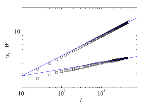
Figure 1: Log-log plots of the width of the product profile $w(t)$ and the width of the depletion zone $W(t)$ vs $t$. The squares are the numerical results for $w(t)$ and the comparison line has slope $\gamma/6$. The circles are the numerical results for $W(t)$ and the line has slope $\gamma/2$.

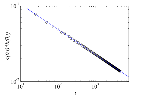
Figure 2: Log-log plots of the product $a(0,t)\times b(0,t)$ vs $t$. The circles are the numerical results and the line has the slope $2\gamma/3$ predicted for this product by our scaling theory.

Here we present a different comparison, namely, between our exact results (where we have them) and our scaling results, and those obtained by direct numerical integration of the reaction-subdiffusion model numerical . This analysis provides an insight not only into the accuracy of the assumptions that enter the scaling analysis, but also into the length of time (rather short, as it turns out) before the asymptotic scaling results are valid. All of our numerical results here have been obtained for the exponent $\gamma=0.5$ and with the parameters $K_{1/2}=k=1$.

Figure 1 shows the width of the product profile, $w(t)$, predicted to grow as $t^{\gamma/6}$, and the width of the depletion zone, $W(t)$, which should grow as $t^{\gamma/2}$ according to our scaling theory. The asymptotic prediction for the former is very good after about $t=100$ and for the latter after about $t=200$. Note that whereas the scaling prediction for $W(t)$ is independent of the form of the reaction term, that of the product profile width $w(t)$ is not.

The product $a(0,t)\times b(0,t)$ is shown in Fig. 2. The agreement between the numerical integration and the scaling result is excellent from the earliest times indicated.

Figure 3 contains a more elaborate set of results showing the space dependence of various quantities at two different times. The triangles pointing upward represent the reactant concentration $a(x,t)$ as a function of position $x$. As expected, this profile is large on the left side of the graph (since reactant $A$ was originally located to the left of the front). The upper curve (solid triangles) corresponds to time $t=1000$ and the lower curve (white triangles), when more of $A$ has already reacted, corresponds to $t=5000$. On the other side and in complete mirror image (because we took both initial concentrations to be equal) are the corresponding results for reactant $B$. The triangles pointing downward represent $b(x,t)$ at the two times, with the same time progression from more reactant to less reactant as time moves on. The quantity that we can directly compare to our theory is the difference profile $u(x,t)=a(x,t)-b(x,t)$. The numerical integration results are represented by the circles. Way to the left of the diagram $u(x,t)\approx a(x,t)$ and way to the right $u(x,t)\approx b(x,t)$, but near the origin both concentrations contribute to $u(x,t)$. The outer solid curve (through solid circles) is the exact result Eq. (11) at $t=1000$ and the inner solid curve is for $t=5000$. The agreement is perfect, as it should be.

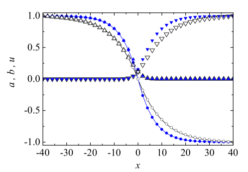
Figure 3: Profiles $a(x,t)$, $b(x,t)$, and the difference profile $u(x,t)=a(x,t)-b(x,t)$ vs $x$ for two different times. The detailed description of this figure is in the text. The theoretical vs numerical comparison is between the circles and the solid curves.

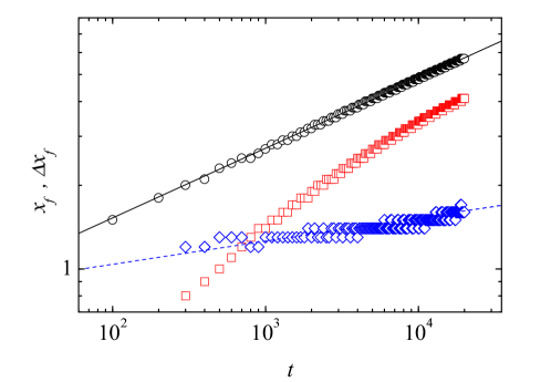
Figure 4: Equimolar point $x_{f}(t)$ vs $t$: circles are numerical integration results and the solid line our exact theoretical values. The squares are the numerical results for the point of maximum product formation, $\hat{x}_{f}(t)$. The difference between the two is represented by the diamonds, and the dashed line is our scaling prediction of slope $\gamma/6$.

Finally, in Fig. 4 we present results for the time dependence of two quantities frequently used to characterize the point of maximum rate of product formation. The point one often sees chosen for this characterization is $x=x_{f}$ such that $a(x_{f},t)=b(x_{f},t)$. This time-dependent equimolar point can be found exactly from the solution Eq. (11), $x_{f}=K_{f}t^{\gamma/2}$, where $K_{f}$ is determined from the equation

$$\frac{2q}{1+q}=H^{10}_{11}\left[K_{f}\left|\begin{array}[]{l}{(1,\frac{\gamma}{2})}\\[4.30554pt] {(0,1)}\end{array}\right.\right].$$ (25)

The circles in the figure are the numerical results for $x_{f}(t)$ with $q=1/2$ and the line is our theoretical prediction with $K_{f}=0.482742\ldots$. A second point (and one that is actually a more accurate characterization of the maximum rate of product formation) is $\hat{x}_{f}$ such that the product $a(\hat{x}_{f},t)b(\hat{x}_{f},t)$ which determines the reaction rate is a maximum. This quantity is more difficult to predict, but we do know that both $x_{f}$ and $\hat{x}_{f}$ are within the reaction zone, which scales as $x/t^{\gamma/6}$. It therefore follows that the distance between these two points should grow as $x_{f}-\hat{x}_{f}\sim t^{\gamma/6}$. But since $x_{f}\sim t^{\gamma/2}$, we conclude that $\hat{x}_{f}\approx x_{f}$ only for times for which their difference is negligible, i.e. only for times such that $t^{-2\gamma/3}\gg 1$. In Fig. 4 the squares are the numerical results for $\hat{x}_{f}(t)$, the diamonds represent the difference $x_{f}-\hat{x}_{f}$, and the dashed line has slope $\gamma/6$. For the two measures to approach closely one has to go to considerably longer times.

IV End notes

We have presented a scaling theory for the evolution of a reaction-subdiffusion front for the annihilation reaction $A+B\to C$. The theory is based on a set of fractional equations in which the diffusion operator is replaced by a Riemann-Liouville operator, and the reaction term is adjusted as well to take into account the slower motion of the reactants. Elsewhere we presented a comparison of our theoretical results with numerical simulations of the process we2 . Here we have presented a detailed comparison of our results with those of numerical integrations of the fractional equations numerical . The familiar rate anomalies of the reaction-diffusion problem are now more pronounced by the slower motion of the reactants, with the result that scaling behaviors are recovered from those of the corresponding diffusive problem with the substitution $t\to t^{\gamma}$.

- (1) E. Kotomin and V. Kuzovkov, Modern Aspects of Diffusion-Controlled Reactions: Cooperative Phenomena in Bimolecular Processes, Elsevier, Amsterdam, 1996.
- (2) K. Lindenberg, P. Argyrakis, and R. Kopelman, “The hierarchies of non-classical regimes for diffusion-limited reactions,” in Fluctuations and Order: The New Synthesis, M. Millonas, ed., p. 171, Springer Verlag, New York, 1996.
- (3) L. Gálfi and Z. Rácz, “Properties of the reaction front in an type reaction-diffusion process,” Phys. Rev. A 38, p. 3151, 1988.
- (4) S. B. Yuste, L. Acedo, and K. Lindenberg, “Reaction front in an reaction-subdiffusion process,” Phys. Rev. E XX, in press.
- (5) S. H. Park, S. Parus, R. Kopelman, and H. Taitelbaum, “Gel-free experiments of reaction-diffusion front kinetics,” Phys. Rev. E 64, p. 055102(R), 2001.
- (6) C. N. Baroud, F. Okkels, L. Ménétrier, and P. Tabeling, “Reaction-diffusion dynamics: Confrontation between theory and experiment in a microfluidic reactor,” Phys. Rev. E 67, p. 060104(R), 2003.
- (7) T. Kostołowicz, K. Dworecki, and S. M. Tabeling, “Measuring subdiffusion parameters,” cond-mat 0309072, 2003.
- (8) J. W. Haus and K. Kehr, “Diffusion in regular and disordered lattices,” Phys. Rep. 150, p. 264, 1987.
- (9) J.-P. Bouchaud and A. Georges, “Anomalous diffusion in disordered media: Statistical mechanisms, models and physical applications,” Phys. Rep. 195, p. 127, 1990.
- (10) E. Barkai, “CTRW pathways to the fractional diffusion equation,” Chem. Phys. 284, p. 13, 2002.
- (11) I. M. Sokolov, A. Blumen, and J. Klafter, “Dynamics of annealed systems under external fields: CTRW and the fractional Fokker-Planck equations,” Europhys. Lett. 56, p. 175, 2001.
- (12) R. Metzler and J. Klafter, “The random walk’s guide to anomalous diffusion: a fractional dynamics approach,” Phys. Rep. 339, p. 1, 2000.
- (13) B. J. West, M. Bologna, and P. Grigolini, Physics of Fractal Operators, Springer, New York, 2003.
- (14) R. Hilfer, Applications of Fractional Calculus in Physics, World Scientific, Singapore, 2000.
- (15) W. R. Schneider and W. Wyss, “Fractional diffusion and wave equations,” J. Math. Phys. 30, p. 134, 1989.
- (16) P. L. Krapivsky, “Diffusion-limited annihilation with initially separated reactants,” Phys. Rev. E 51, p. 4774, 1995.
- (17) S. J. Cornell, M. Droz, and B. Chopard, “Role of fluctuations for inhomogeneous reaction-diffusion phenomena,” Phys. Rev. A 44, p. 4826, 1991.
- (18) A. M. Mathai and R. K. Saxena, The H-function with Applications in Statistics and Other Disciplines, John Wiley and Sons, New York, 1978.
- (19) B. I. Henry and S. L. Wearne, “Fractional reaction-diffusion,” Physica A 276, p. 448, 2000.
- (20) M. O. Vlad and J. Ross, “Systematic derivation of reaction-diffusion equations with distributed delays and relations to fractional reaction-diffusion equations and hyperbolic transport equations: Application to the theory of neolithic transition,” Phys. Rev. E 66, p. 061908, 2002.
- (21) S. Fedotov and V. Méndez, “Continuous-time random walks and traveling fronts,” Phys. Rev. E 66, p. 061908, 2002.
- (22) J. Sung, E. Barkai, R. J. Silbey, and S. Lee, “Fractional dynamics approach to diffusion-assisted reactions in disordered media,” J. Chem. Phys. 116, p. 2338, 2002.
- (23) K. Seki, M. Wojcik, and M. Tachiya, “Fractional reaction-diffusion equation,” J. Chem. Phys. 119, p. 2165, 2003.
- (24) K. Seki, M. Wojcik, and M. Tachiya, “Recombination kinetics in subdiffusive media,” J. Chem. Phys. 119, p. 7525, 2003.
- (25) S. B. Yuste and L. Acedo, “On an explicit finite difference method for fractional diffusion equations,” SIAM J. Num. Anal. 52, p. 1862-74, 2005.