Inelastic quantum transport in a ladder model: Measurements of DNA conduction and comparison to theory

Abstract

We investigate quantum transport characteristics of a ladder model, which effectively mimics the topology of a double-stranded DNA molecule. We consider the interaction of tunneling charges with a selected internal vibrational degree of freedom and discuss its influence on the structure of the current-voltage characteristics. Further, molecule-electrode contact effects are shown to dramatically affect the orders of magnitude of the current. Recent electrical transport measurements on suspended DNA oligomers with a complex base-pair sequence, revealing strikingly high currents, are also presented and used as a reference point for the theoretical modeling. A semi-quantitative description of the measured $I$-$V$ curves is achieved, suggesting that the coupling to vibrational excitations plays an important role in DNA conduction.

I Introduction

The past decade has seen an extraordinary progress in the field of molecular electronics. The possibility of using single molecules or molecular groups as the basic building units of electronic circuits has considerably triggered the refinement of experimental techniques. As a result, transport signatures of individual molecules have been successfully probed and exciting physical effects like rectification, Coulomb blockade, and the Kondo effect among others have been demonstrated, see e.g. Ref. [Cuniberti et al., 2005] for a recent review of the field.

Within the class of biopolymers, DNA is expected to play an outstanding role in molecular electronics. This is mainly due to its unique self-assembling and self-recognition properties, which are essential for its performance as carrier of the genetic code, and may be further exploited in the design of electronic circuits. Keren et al. (2003); Mertig et al. (1999) A related important issue is to clarify if DNA in some of its possible conformations can carry an electric current or not. In other words, if it could also be applied as a wiring system. In the early 1990’s charge transfer experiments in natural DNA in solution showed unexpected high charge transfer rates, Treadway et al. (2002); Murphy et al. (1993) thus suggesting that DNA might support charge transport. However, electrical transport experiments carried out on single DNA molecules displayed a variety of possible behaviors: insulating, Braun et al. (1998); Storm et al. (2001) semiconducting, Porath et al. (2000); Cohen et al. (2005, 2006, 2004) and ohmic-like. Yoo et al. (2001); Xu et al. (2004) This can apparently be traced back to the high sensitivity of charge propagation in this molecule to extrinsic (interaction with hard substrates, metal-molecule contacts, aqueous environment) as well as intrinsic (dynamical structure fluctuations, base-pair sequence) factors. Recently, experiments on single poly(GC) oligomers in aqueous solution Xu et al. (2004) as well as on single suspended DNA with a complex base sequence Cohen et al. (2005, 2006) have shown unexpectedly high currents of the order of 100-200 nA. These results strongly suggest that DNA molecules may indeed support rather high electrical currents if the appropriate conditions are warranted. The theoretical interpretation of these experiments and, in a more general context, the mechanism(s) for charge transport in DNA have not , however, been revealed so far.

Both ab initio calculations Artacho et al. (2003); Calzolari et al. (2002); Felice et al. (2004); Gervasio et al. (2002); Barnett et al. (2001); Hübsch et al. (2005); Starikov (2003, 2005); Adessi et al. (2003); Mehrez and Anantram (2005) as well as model-based Hamiltonian approaches Cuniberti et al. (2002); Jortner et al. (1998); Jortner and Bixon (2002); Roche et al. (2003); Roche (2003); Unge and Stafstrom (2003); Hennig et al. (2004); Jortner and Bixon (2005); Apalkov and Chakraborty (2005a, b); Gutierrez et al. (2005a, b); Kohler et al. (2005); Yamada et al. (2004); D’Orsogna and Bruinsma (2003) have been recently discussed. Though the former can give in principle a detailed account of the electronic and structural properties of DNA, the huge complexity of the molecule and the diversity of interactions present in it (internal as well as with the counterions and hydration shells) precludes a full systematic first principles treatment of electron transport for realistic molecule lengths, this becoming even harder if the dynamic interaction with vibrational degrees of freedom is considered. Thus, Hamiltonian approaches can play a complementary role by addressing single factors that influence charge transport in DNA.

In this paper, we will address the influence of vibrational excitations (vibrons) on the quantum transport signatures of a ladder model, which we use to mimic the double-strand structure of DNA oligomers. As a reference for our calculations we will take the previously mentioned experiments on single suspended DNA molecules with a complex base-pair sequence. Cohen et al. (2005, 2006) Our main goal is to disclose within a generic Hamiltonian model the influence of different parameters on the charge transport properties: the system-electrode coupling, the strength of the charge-vibron coupling, and the vibron frequency. Our model suggests that strong coupling to vibrational degrees of freedom may lead to an enhancement of the zero-current gap, which is a result of a vibron blockade effect. Koch and von Oppen (2005) Further, asymmetries in the ladder-lead coupling have a drastic effect on the absolute values of the current. Finally, we show that a two-vibron model can describe the shape of the experimental $I$-$V$ curves of Ref. [Cohen et al., 2005], suggesting that interaction with vibrational degrees of freedom may give a non-negligible contribution to the measured currents. Obviously, other factors related e.g. to the specific metal-molecule interface atomic structure which govern the efficiency of charge injection, or the potential profile along the molecule can give important contributions. They can be taken into account by a more realistic, fully self-consistent treatment of the problem, which lies outside the scope of the present study.

In the next section we briefly present the experimental results. In Sec. III.A the model Hamiltonian is introduced and the relevant parameters are defined. The theoretical formalism is discussed in Sec. III.B. Finally, the results are presented and discussed in Sec. IV.

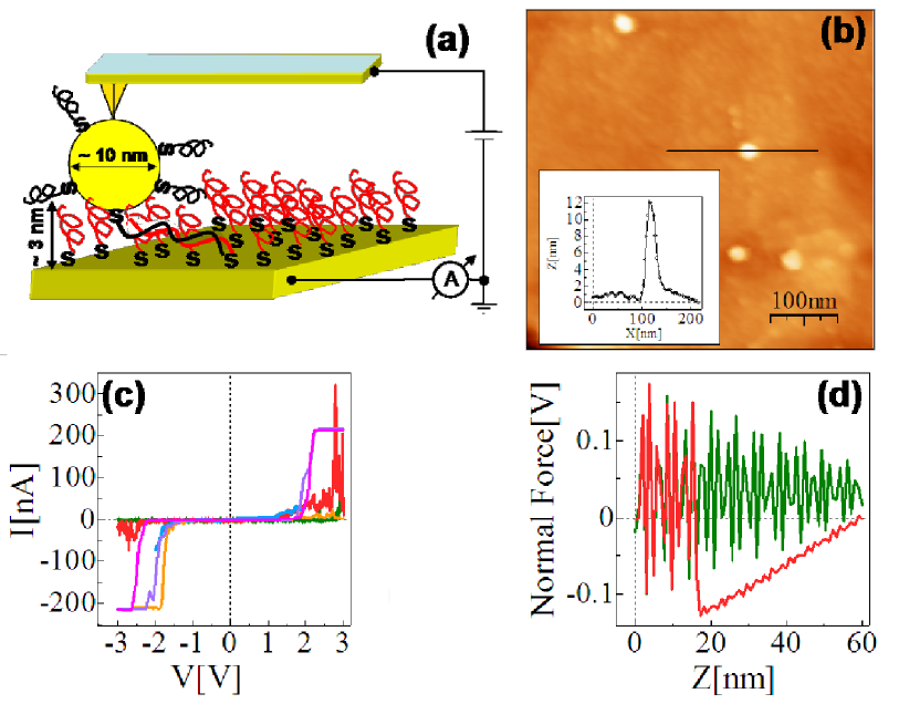
Figure 1: (a) Scheme (not drawn to scale) of the experimental setup showing dithiolated dsDNA (thicker lines for clarity) chemically bonded to two metal electrodes (upper - GNP, lower - gold surface), supported by a monolayer of thiolated ssDNA. (b) AFM topography image showing top view of the sample. Several GNPs are clearly seen on the background of the ssDNA monolayer. The GNPs mark the position of the hybridized dsDNA. The inset is a height profile of the GNP lying on the ssDNA surface. (c) Collection of I-V curves from different samples. In some other cases we measured smaller or no voltage gap. Note that several curves show saturation of the current amplifier at 220 nA. (d) An F-Z curve of one of the curves in (c), (green-forward, red-backward) demonstrating the tip-GNP adhesion (red line) without pressing the GNP through the monolayer. The I-V is recorded at the closest point of the tip to the GNP without pressing it through the ssDNA monolayer.

II Experimental aspects

Detailed description of the sample preparation is reported elsewhere. Cohen et al. (2005, 2006, 2004) Briefly, a thiolated 26 bases long single-stranded DNA (ssDNA) with a complex sequence was adsorbed on a clean flat annealed gold surface to create a dense monolayer. The ssDNA molecules had a thiol-modified linker end group (CH₂)₃-SH at the 3’-end. The sequence of the ssDNA that was adsorbed on the gold surface in 0.4 M phosphate buffer with 0.4 M NaCl is 5’-CAT TAA TGC TAT GCA GAA AAT CTT AG-3’-(CH₂)₃-SH. The surface density of the monolayer on the gold was appropriate for hybridization with complementary thiolated ssDNA that were separately adsorbed on 10 nm gold nanoparticles (GNPs) through another thiol group at their 3’-end by a (CH₂)₃-SH group. The monolayer serves also as an insulating support to the GNPs. Cohen et al. (2005, 2006, 2004) Direct measurements by conductive atomic force microscope (cAFM) with tip-sample bias of up to 3 V confirmed that the monolayer was insulating.  Cohen et al. (2005, 2006) The double-strand DNA (dsDNA) hybridization was done at ambient conditions in the presence of 25 mM Tris buffer with 0.4 M NaCl. Before AFM characterization and electrical measurements the samples were thoroughly rinsed to remove excess salts.

The measurements were done with a commercial AFM (Nanotec Electronica S.L. Madrid) in dynamic mode de Pablo et al. (2000) to avoid damage to the sample and the metal coated tip. Rectangular cantilevers with Pyramidal tips (Olympus, OMCL-RC800PSA, Atomic Force F$\&$E GmbH, spring constant of 0.3 to 0.7 N/m and resonance frequency of 75 to 80 KHz) were used in order to perform combined force-distance (F-Z) and current-voltage (I-V) curves with a minimal load on the sample. For the electrical measurements the tips were sputter coated by Au/Pd that increased their spring constant to about 1 N/m and lowered their resonance frequency to 50-70 KHz. Throughout the measurements the cantilever was oscillated close to its resonance frequency and feedback was performed on the amplitude of its vibrations. Fig. 1(a) shows a schematic view of the sample and set-up. Fig. 1(b) is an AFM image showing several GNPs, indicating the position of the hybridized dsDNA on the background of the ssDNA monolayer. A line profile along one of the 10 nm GNPs implies that the 26 bp dsDNA, which is $\sim$9 nm long, is not protruding vertically out of the $\sim 3-4$ nm thick ssDNA monolayer and is probably tilted and lying on the surface of the ssDNA monolayer. The electrical I-V curves (Fig. 1(c)) were recorded while the GNP was contacted during an F-Z curve by the metal covered tip without pressing the tip onto the GNP. This was done by applying a feedback on the tip oscillation amplitudes, while approaching the GNP, that enabled to stop the tip movement towards the GNP just before the jump to contact, as demonstrated in the F-Z curve showed in Fig. 1(d).

The current voltage curves, shown in Fig 1(c), demonstrate in a clear and reproducible way, the ability of $\sim$9 nm long dsDNA to conduct relatively high currents ($>$ 200 nA), when the molecule is not attached to a hard surface along its backbone and when charge can be injected efficiently through a chemical bond. Such behavior was measured for many dsDNA molecules on tens of samples and with various tips and humidity conditions, with similar results. Cohen et al. (2005) This behavior was also measured in the absence of the GNPs using a different technique. Cohen et al. (2006)

III Theoretical aspects

III.1 Model Hamiltonian

Our aim is to formulate a minimal model taking into account the double-strand structure of DNA. Hence, we do not consider the full complexity of the DNA electronic structure. We neglect environmental effects and assume that charge transport will mainly take place along the base-pair stack. We further adopt the perspective that to describe low-energy quantum transport within a single-particle picture, only the frontier $\pi$ orbitals of the base pairs are relevant. We will then consider a planar ladder model with a single orbital per lattice site within a nearest-neighbor tight-binding picture. In this sense, we are neglecting helical effects arising from the real structure of the DNA. We assume that these and similar effects may have already renormalized the electronic parameters. We will focus in this paper on the experimentally relevantCohen et al. (2005) base-pair sequence X=5’-CAT TAA TGC TAT GCA GAA AAT CTT AG-3’, see Fig. 2 and the foregoing section. It is worth mentioning that ladder models have been previously used to study quantum transport in DNA duplexes. Yi (2003); Yamada (2004); Yamada et al. (2004); Klotsa et al. (2005); Caetano and Schulz (2005); Wang and Chakraborty (2006)

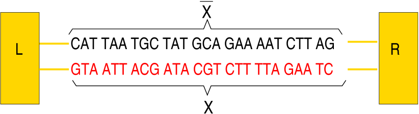
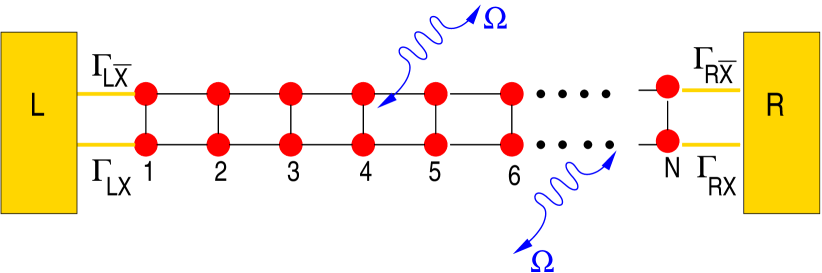
Figure 2: Upper panel: Schematic representation of the double-strand DNA with the experimentally relevant base-pair sequence. Cohen et al. (2005) The (CH₂)₃-SH linker groups are omitted for simplicity (see the text for details). Lower panel: Two-legs ladder used to mimic the double-strand structure of a DNA molecule. L and R refer to left and right electrodes, respectively. The coupling terms to the electrodes $\Gamma_{\ell,\alpha},\ell=$X,$\bar{X}$, $\alpha=$L,R are assumed to be energy-independent constants (wide -band limit, see the text for details).

The Hamilton operator describing the ladder and its coupling to left (L) and right (R) electronic reservoirs is given by:

$$\cal{H}_{\rm el} = \sum_{\rm{r}=X,\bar{X}}\sum_{\ell}\epsilon_{\rm{r},\ell}b^{\dagger}_{\rm{r},\ell}b_{\rm{r},\ell}$$

$$- \sum_{\rm{r}=X,\bar{X}}\sum_{\ell}t_{\rm{r},\ell,\ell+1}[b^{\dagger}_{\rm{r},\ell}b_{\rm{r},\ell+1}+\textrm{h.c.}]$$

$$- \sum_{\ell}t_{\perp,\ell}[b^{\dagger}_{\rm{X},\ell}b_{\rm{\bar{X}},\ell}+\textrm{h.c.}]$$

$$+ \sum_{{\bf k}\in L}[t_{{\bf k},X}c^{\dagger}_{{\bf k}}b_{X,1}+\textrm{h.c.}]+\sum_{{\bf k}\in L}[t_{{\bf k},\bar{X}}c^{\dagger}_{{\bf k}}b_{\bar{X},1}+\textrm{h.c.}]$$

$$+ \sum_{{\bf k}\in R}[t_{{\bf k},X}c^{\dagger}_{{\bf k}}b_{X,N}+\textrm{h.c.}]+\sum_{{\bf k}\in R}[t_{{\bf k},\bar{X}}c^{\dagger}_{{\bf k}}b_{\bar{X},N}+\textrm{h.c.}]$$

In the previous expression, $X,\bar{X}$ refer to the two legs of the ladder, $\epsilon_{\rm{r},\ell}$ are energies at site $\ell$ on leg $\rm{r}$, $t_{\rm{r},\ell,\ell+1}$ are the corresponding nearest-neighbor electronic hopping integrals along the two strands while $t_{\perp,\ell}$ describes the inter-strand hopping. In order to obtain estimates of onsite energies and hopping integrals, ab initio calculations are obviously the most reliable reference point. Recently, Mehrez and Anantram Mehrez and Anantram (2005) carried out a careful analysis of a hierarchy of tight-binding models that gave effective onsite energies and hopping parameters for Poly(GC) and Poly(AT) molecules. We will use these values as a reference point in part of our discussion and take the onsite energies as the LUMO energies given in Ref. [Mehrez and Anantram, 2005]: $\epsilon_{\rm G}=1.14\,$eV,$\epsilon_{\rm C}=-1.06\,$eV, $\epsilon_{\rm A}=0.26\,$eV,$\epsilon_{\rm T}=-0.93\,$eV. We are thus considering electron transport, although hole transport can be dealt with in a similar way by choosing the HOMO instead of the LUMO energies. Other choices e. g. the ionization potentials of the base pairs are also possible; Roche (2003) they are expected to only change our results quantitatively. More difficult is the choice of the intra- and inter-strand electronic transfer integrals. They will be more sensitive to the specific base sequence considered. For the sake of simplicity and in order to reduce the number of model parameters we have adopted a simple parameterization taking a homogeneous hopping along both legs, i. e. $t_{\rm{r},\ell,\ell+1}=t_{\rm{X}}=t_{\rm{\bar{X}}}=t\sim 0.25-0.27$ eV and $t_{\perp,\ell}=t_{X\bar{X}}\sim$0.2-0.3 eV. Though calculations Mehrez and Anantram (2005); Voityuk et al. (2000) show that the inter-strand hopping is usually very small, $\sim$ few meV, we do not consider the hopping integrals as bare tight-binding parameters but as effective ones, thus keeping some freedom in the choice of their specific values. Electronic correlations Yi (2003) or structural fluctuations mediated by the coupling to other vibrational degrees of freedom Voityuk et al. (2001) can lead to a strong renormalization of the bare electronic coupling.

The interaction with the electronic reservoirs will be described in the most simple way by invoking the wide-band approximation, i. e. neglecting the energy dependence of the leads’ self-energies (see below). To model the coupling to vibrational degrees of freedom we consider the case of long-wave length optical modes with constant frequencies $\Omega_{\alpha}$, e. g. small-q torsional modes and assume they couple to the total charge density operator $N=\sum_{\rm r,\ell}n_{\rm r,\ell}$ of the ladder. This approximation can be justified for long-wave length distortions. In other words, the strength of the electron-vibron interaction $\lambda$ is assumed to be site-independent. Moreover, we will not consider in this study non-local coupling to vibrational excitations. Though this interaction can give an important contribution to the modulation of the inter-site electronic hopping, its inclusion would increase the complexity of the model and the number of free parameters. Such effects deserve a separate investigation; research along these lines has been recently presented by other authors. Grozema et al. (2002); Berlin et al. (2001); Grozema et al. (2001); Palmero et al. (2004); Senthilkumar et al. (2004) The total Hamiltonian thus reads:

$${\cal{H}}={\cal{H}_{\rm el}}+\sum_{\alpha}\Omega_{\alpha}B^{\dagger}_{\alpha}B_{\alpha}+\sum_{\rm{r},\ell,\alpha}\lambda_{\alpha}b^{\dagger}_{\rm{r},\ell}b_{\rm{r},\ell}(B_{\alpha}+B^{\dagger}_{\alpha})$$ (1)

III.2 Green function techniques

In this section we present the theoretical approach to deal with electrical transport properties in the presence of electron-vibron coupling. Taking as a starting point the Hamiltonian of Eq. 1, we perform a Lang-Firsov (LF) unitary transformation Mahan (2000) in order to eliminate the electron-vibron interaction. The LF-generator is given by ${\cal U}=\exp[-\sum_{\alpha,\rm{r},\ell}g_{\alpha}b^{\dagger}_{\rm{r},\ell}b_{\rm{r},\ell}(B_{\alpha}-B^{\dagger}_{\alpha})]$, which is basically a shift operator for the harmonic oscillator position. The parameter $g_{\alpha}=\lambda_{\alpha}/\Omega_{\alpha}$ gives an effective measure of the electron-vibron coupling strength. In the resulting Hamiltonian, the onsite energies $\epsilon_{\rm{r},\ell}$ are shifted to $\epsilon_{\rm{r},\ell}-\Delta$ with $\Delta=\sum_{\alpha}\lambda^{2}_{\alpha}/\Omega_{\alpha}$ being the polaron shift. There is an additional renormalization of the tunneling Hamiltonian, but we will not consider it explicitly, since we will assume a regime (within the wide-band approximation in the leads’ spectral densities) where the effective broadening $\sim\Gamma$ arising from the coupling to the leads is bigger than the polaron formation energy $\sim\lambda^{2}/\Omega$ . As shown in Ref. [Hewson and Newns, 1979] in this special case the tunneling renormalization can be approximately neglected.

Concerning the transport problem, we can use the standard current expression for lead $p$=L,R as derived e.g. by Meir and Wingreen. Meir and Wingreen (1992)

$$I_{p}=\frac{2\textrm{i}\,e}{h}\int dE\,\textrm{Tr}[\Gamma_{\textrm{p}}\{f_{\textrm{p}}(G^{>}-G^{<})+G^{<}\}],$$ (2)

and then perform the LF unitary transformation under the trace going over to the transformed Green functions. In the previous equation, $\Gamma_{\textrm{p}}(E)=\textrm{i}\,\,(\Sigma_{\textrm{p}}(E)-\Sigma^{\dagger}_{\textrm{p}}(E))$ are the leads’ spectral functions, $f_{\textrm{p}}(E)=f(E-\mu_{\textrm{p}})$ is the Fermi function of the p-lead and $\mu_{\textrm{p}=\textrm{L}}=E_{\rm F}+eV/2\;(\mu_{\textrm{p}=\textrm{R}}=E_{\rm F}-eV/2)$ are the corresponding electrochemical potentials. We assume hereby a symmetrically applied bias. Within the wide-band limit in the electrodes’ spectral densities, we introduce the following $2N\times 2N$ ladder-lead energy-independent coupling matrices:

$$(\Gamma_{\textrm{L}})_{nm}=\left\{\begin{array}[]{r@ { \quad\textrm{if} \quad}l}\Gamma_{L,X}\delta_{n,1}\delta_{m,1}&n,m\in X\\ \Gamma_{L,\bar{X}}\delta_{n,1}\delta_{m,1}&n,m\in\bar{X}\\ 0&\neq 1\end{array}\right.$$

$$(\Gamma_{\textrm{R}})_{nm}=\left\{\begin{array}[]{r@ { \quad\textrm{if} \quad}l}\Gamma_{R,X}\delta_{n,N}\delta_{m,N}&n,m\in X\\ \Gamma_{R,\bar{X}}\delta_{n,N}\delta_{m,N}&n,m\in\bar{X}\\ 0&n,m\neq N\end{array}\right.$$

We remark at this point that these coupling terms also include effectively the (CH₂)₃-SH linkers used in the experiments to attach the DNA molecule to the metallic electrodes..

Let’s define the fermionic vector operator (see Fig. 2 for reference):

$$\Psi^{\dagger}=(b_{X,1}\,b_{X,2}\,\cdots b_{X,N}\,b_{\bar{X},1}\,\cdots\,b_{\bar{X},N}).$$ (3)

The lesser- and greater-matrix Green function (GF) are then defined as:

$$G^{>}(t) = -\frac{\textrm{i}\,}{\hbar}\left\langle\Psi(t)\Psi^{\dagger}(0)\right\rangle,$$ (4)

$$G^{<}(t) = \frac{\textrm{i}\,}{\hbar}\left\langle\Psi^{\dagger}(0)\Psi(t)\right\rangle.$$

Since Eq. 2 does not explicitly contain information on the specific structure of the “molecular” Hamiltonian, we can now transform the lesser- and greater-GF as well as the lead spectral functions to the polaron representation. The operator $\Psi$ transforms according to $\bar{\Psi}={\cal U}\Psi{\cal U}^{\dagger}=\Psi{\cal X}$, where ${\cal X}=\exp[\sum_{\alpha}(\lambda_{\alpha}/\Omega_{\alpha})(B_{\alpha}-B^{\dagger}_{\alpha})]$. Thus, we obtain $\bar{G}^{>}(t)=-(\textrm{i}\,/\hbar)\left\langle\Psi(t){\cal X}(t)\,\Psi^{\dagger}(0){\cal X}^{\dagger}(0)\right\rangle$ and similar for $\bar{G}^{<}(t)$. Strictly speaking, a further direct decoupling of the foregoing expression into purely fermionic and vibronic components, as is usual in the independent vibron model Mahan (2000) is not possible, since the transformed tunneling Hamiltonian contains both types of operators and hence, the transformed canonical density operator does not factorize into separate fermion and vibron density operators. However, for the case considered here, where vibron-induced renormalization effects of the tunneling amplitudes are not taken into account, the decoupling is still approximately possible. We thus obtain:

$$\bar{G}^{>}(t) = -\frac{\textrm{i}\,}{\hbar}\left\langle\Psi(t){\cal X}(t)\,\Psi^{\dagger}(0){\cal X}^{\dagger}(0)\right\rangle$$

$$\approx -\frac{\textrm{i}\,}{\hbar}\left\langle\Psi(t)\Psi^{\dagger}(0)\right\rangle_{el}\left\langle{\cal X}(t){\cal X}^{\dagger}(0)\right\rangle_{B}$$

$$= G^{>}(t)\left\langle{\cal X}(t){\cal X}^{\dagger}(0)\right\rangle_{B}=G^{>}(t)e^{-\Phi(t)}.$$

A similar expression holds for the lesser-than GF by changing the time argument $t$ by $-t$ in $\Phi(t)$. We note that $\Phi(t)$ satisfies the symmetry relations: $\Phi(-t)=\Phi^{\dagger}(t)$.

III.3 Single-vibron case

In the case of dispersionless modes, the vibron correlation function $\Phi(t)$ can be evaluated exactly and reads: Mahan (2000)

$$e^{-\Phi(t)}=e^{-g^{2}(2N+1)}\,\sum^{\infty}_{n=-\infty}I_{n}(\tau)e^{\beta\Omega n/2}e^{-\textrm{i}\,n\Omega t},$$ (5)

where $\tau=2g^{2}\sqrt{N(N+1)}$ and $g=\lambda/\Omega$. Using this expression, one easily finds for the Fourier transformed lesser and greater GFs:

$$\bar{G}^{<(>)}(E) = \sum^{\infty}_{n=-\infty}\phi_{n}(\tau)G^{<(>)}(E+(-)n\Omega),$$ (6)

$$\phi_{n}(\tau) = e^{{-g^{2}(2N+1)}}\;\times I_{n}(\tau)\;e^{{\beta\Omega\,n/2}}.$$

where $+(-)$ corresponds to $<(>)$. The bare lesser- and greater-GF can now be obtained from the kinetic equation $G^{<(>)}=G^{r}(\Sigma^{<(>)}_{\textrm{L}}+\Sigma^{<(>)}_{\textrm{R}})G^{a}$, since the full electron-vibron coupling is already contained in the prefactor function $\phi_{n}(\tau)$. The leads self-energy matrices $\Sigma^{<}_{\textrm{p}},\Sigma^{>}_{\textrm{p}}$ are given in the wide-band limit by $\textrm{i}\,f_{\textrm{p}}(E)\Gamma_{\textrm{p}}$ and $-\textrm{i}\,(1-f_{\textrm{p}}(E))\Gamma_{\textrm{p}}$, respectively. Using these expressions, the total symmetrized current in the stationary state $J_{\rm T}=(J_{\textrm{L}}-J_{\textrm{R}})/2$ is given by (see Appendix):

$$J_{\rm T} = \frac{e}{2h}\sum^{\infty}_{n=-\infty}\phi_{n}(\tau)\int dE\,\{[f_{\textrm{L}}(E)\,(1-f_{\textrm{R}}(E-n\Omega))$$ (8)

$$- f_{\textrm{R}}(E)\,(1-f_{\textrm{L}}(E-n\Omega))]\,t(E-n\Omega)$$

$$+ [f_{\textrm{L}}(E+n\Omega)\,(1-f_{\textrm{R}}(E))$$

$$- f_{\textrm{R}}(E+n\Omega)\,(1-f_{\textrm{L}}(E))]\,t(E+n\Omega)\},$$

where $t(z)=\textrm{Tr}[\Gamma_{\textrm{R}}G^{\textrm{r}}(z)\Gamma_{\textrm{L}}G^{\textrm{a}}(z)]$ is the conventional expression for the transmission coefficient in terms of the molecular Green function $G(E)$, which satisfies the Dyson-equation: $G^{-1}=G^{-1}_{0}-\Sigma_{\textrm{L}}-\Sigma_{\textrm{R}}$. The above result for the current has a clear physical interpretation. So, e.g. a term like $f_{\textrm{L}}(E)\,(1-f_{\textrm{R}}(E-n\Omega))t(E-n\Omega)$ describes an electron in the left lead which tunnels into the molecular region, emits $n$ vibrons of frequency $\Omega$ and tunnels out into the right lead. However, it can only go into empty states, hence the Pauli blocking factor $(1-f_{\textrm{R}}(E-n\Omega))$. Other terms can be interpreted along the same lines, when one additionally substitutes electrons by holes.

Finally, the spectral density $A(E,V)$ is defined as:

$$A(E,V) = \textrm{i}\,\,[\bar{G}^{>}(E)-\bar{G}^{<}(E)]$$

$$= \textrm{i}\,\,\sum_{n}\phi_{n}(\tau)\,[G^{>}(E-n\Omega)-{G}^{<}(E+n\Omega)]$$

IV Results

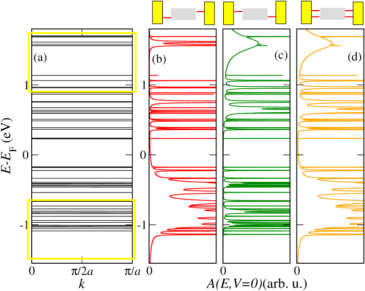
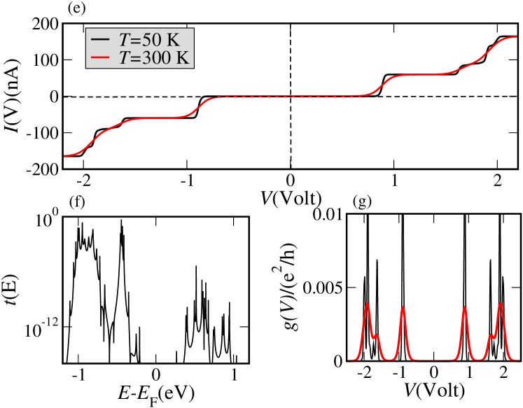
Figure 3: (a) Tight-binding electronic band structure of an infinite DNA system, obtained by a periodic repetition of the 26-base sequence of Ref. [Cohen et al., 2005]. Notice the strongly fragmented band structure with very flat bands. The open yellow rectangles indicate for reference the approximate position of the bands for a periodic poly(GC) oligomer. (b)-(d) spectral density $A(E,V=0)$, which at zero voltage coincides with the projected density of states onto the molecular region, for the finite size DNA chain contacted in different ways by left and right electrodes, see Fig. 2: (b)$\Gamma_{L,X}=\Gamma_{R,\bar{X}}=0,\Gamma_{L,\bar{X}}=\Gamma_{R,X}=250\,$meV, (c) $\Gamma_{L,X}=\Gamma_{R,\bar{X}}=250\,$meV,$\Gamma_{L,\bar{X}}=\Gamma_{R,X}=0\,$meV, (d) $\Gamma_{L,X}=\Gamma_{R,\bar{X}}=\Gamma_{L,\bar{X}}=\Gamma_{R,X}=250\,$meV. The onsite energies were set at the LUMO values reported in Ref. [Mehrez and Anantram, 2005] and the hopping parameters were set to $t_{X}=t_{\bar{X}}=t=0.27\,$eV, $t_{X\bar{X}}=0.25\,$eV. (e) $I$-$V$ characteristics for two different temperatures and the contact situation (b); (f) corresponding transmission function $t(E)$ and (g) differential conductance $g(V)$.

In Fig. 3(a) we first show the electronic band structure of an infinite periodic array of the 26-base-pairs DNA molecule without considering charge-vibron interactions. The unit cell thus contains 2$\times$26 sites. Due to the large unit cell and since the electronic hopping integrals are roughly a factor four smaller than the onsite energies, one gets a strongly fragmented electronic spectrum with very flat bands. We may thus rather speak of valence and conduction manifolds as of true dense electronic bands. Felice et al. (2002) The band gap $\Delta$ of about 0.3 eV is considerably smaller than that obtained in the periodic poly(GC) ladder when using the same parameterization, $\Delta_{\rm{GC}}\sim 2.0$ eV. In Fig. 3(a) we also show schematically the positions of the conduction and valence manifolds of the periodic poly(GC) system (open rectangles). We note in passing that similar small gaps have been estimated in experiments on $\lambda$-DNA Tran et al. (2000) and in bundles Rakitin et al. (2001). A direct comparison to our results is however not possible due to the different experimental conditions and length scales probed in these investigations. Figs. 3(b)-(d) show the spectral density at zero voltage of the finite DNA ladder contacted by electrodes in three different ways: (b) only the 3’-ends, (c) only the 5’-ends, and (d) all four ends of the double-strand are contacted. Though the general effect consists in broadening of the electronic manifolds, we also see that depending on the way the molecule is contacted to the leads the electronic states will be affected in different ways. Thus e.g. states around 1.7 eV above the Fermi level are considerably more broadened than states closer to E${}_{\textrm{F}}$. Figs. 3(e)-(g) show the current, transmission and differential conductance for one of the typical contact situations (case (b)). The irregular step-like structure in the current-voltage characteristics is reflecting the fragmented electronic structure of the system. Notice that despite the small gap found in the band structure resp. DOS, a large ($\sim 2$ V) zero-current gap is seen in the $I$-$V$ characteristics. The reason is that many of the states close to the band gap have a very low transmission probability (are highly localized) as a result of the random base sequence, see $t(E)$ in Fig. 3(f), so that they do not contribute to transport. The effect of the temperature is only to smooth the current and the differential conductance, as expected. We remark at this point that the absolute values of the current can be dramatically modified by the way the molecule is contacted by the electrodes (see below).

We now consider the coupling to vibrational degrees of freedom in the ladder. The probability of opening inelastic transport channels by emission or absorption of $n$ vibrons becomes higher with increasing thermal energy $k_{\textrm{B}}T$ and/or electron-vibron coupling $g$. As a result, the spectral density $A(E)$ will consist of a series of elastic peaks (corresponding to $n=0$) plus vibron satellites ($n\neq 0$). If the separation between contiguous molecular eigenstates is of the order of the vibron frequency $\Omega$, then the satellites corresponding to a given molecular state will not be clearly separated from the elastic peaks but will overlap with those of nearby molecular states leading to an effective broadening of the spectrum and possibly to complex interference effects.

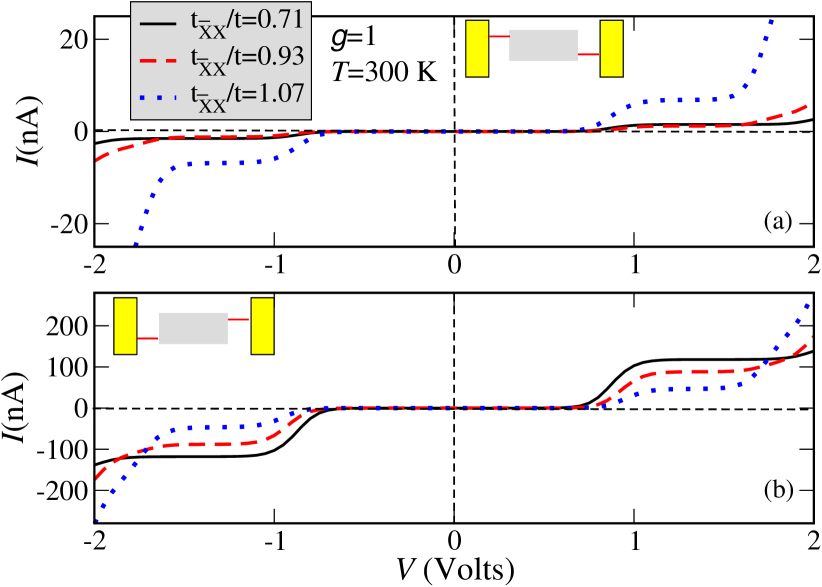
Figure 4: $I$-$V$ characteristics for different values of the reduced inter-strand hopping $t_{X\bar{X}}/t$ in DNA₂₆ for a fixed electron-vibron coupling strength $g=1$. Upper and lower panels correspond to two different (asymmetric) ways of coupling the ladder to the electrodes: (a) $\Gamma_{L,X}=\Gamma_{R,\bar{X}}=0,\Gamma_{L,\bar{X}}=\Gamma_{R,X}=250\,$meV and (b)$\Gamma_{L,\bar{X}}=\Gamma_{R,X}=0,\Gamma_{L,X}=\Gamma_{R,\bar{X}}=250\,$meV. Notice the strong variation in the current when going from case (a) to case (b).

The influence of the transverse electronic hopping and the leads-ladder coupling on the current is shown in Fig 4. The inter-strand hopping turns out to be crucial in determining the absolute values of the current. In the general case of symmetric coupling ($\Gamma_{L,X}=\Gamma_{R,X}=\Gamma_{L,\bar{X}}=\Gamma_{R,\bar{X}}$), a charge propagating along one of the strands will see a rather disordered system, so that a non-zero inter-strand hopping may increase the delocalization of the electronic states. The effect should be more obvious in the case of asymmetric coupling (a) $\Gamma_{L,\bar{X}}=\Gamma_{R,X}\neq 0,\Gamma_{L,X}=\Gamma_{R,\bar{X}}=0$, and (b) $\Gamma_{L,\bar{X}}=\Gamma_{R,X}=0,\Gamma_{L,X}=\Gamma_{R,\bar{X}}\neq 0$ since now there is a single pathway for an electron tunneling from the electrodes into the ladder, e.g. $L\to X\to\bar{X}\to R$. We thus see in Fig. 4 that relative small variations of $t_{X\bar{X}}$ considerably modify the current. We note in passing that recent transport measurements on DNA oligonucleotides have displayed considerable differences in the conductance of single- vs. double-stranded DNA, thus suggesting that, apart from other factors, inter-strand interactions may play a role in controlling charge transport. Zalinge et al. (2006)

Our above results are, moreover, very sensitive to the way the ladder is coupled to the electrodes, as seen from the upper and lower panels of Fig. 4. These cases are related respectively to the situation where only the 5’-end (a) or only the 3’-end sites (b) of the ladder have non-zero coupling to the electrodes, see Fig. 2 for reference. Notice that (b) would correspond to the experimental contact geometry in Ref. [Cohen et al., 2005] where only the 3’-end of each strand in the double helix is connected $-$ via the linker groups $-$ to one of the electrodes (Au-substrate and GNP). Configuration (b) also leads to considerably higher currents than the case (a).

More generic assertions require, however, a detailed atomistic investigation of the DNA-metal contact topology and base-pairs energetics, which goes beyond the scope of this study.

Fig. 5 shows the influence of the coupling to the vibron mode on the magnitude of the current and of the zero-current gap. The slope of the $I$-$V$ curves is considerably reduced with increasing $g$. The corresponding spectral densities at $V\sim 1.5$ Volt, see Fig. 5, lower panel, show broadening due to the emergence of an increasing number of vibron satellites (inelastic channels) with larger coupling, but at the same time a redistribution of spectral weights takes place. This is simply the result of the sum rule $\int dE\,A(E)=2\pi$. The reason for the current reduction can be qualitatively understood by looking at the spectral density. The reduction in the intensity of $A(E)$ will clearly lead to a reduction in the current at a fixed voltage, since it is basically the area under $A(E,V=\textrm{const.})$ within the energy window $\left[E_{\textrm{F}}-eV/2,E_{\textrm{F}}+eV/2\right]$ which really matters. Notice also the increase of the zero-current gap with increasing electron-vibron coupling (vibron blockade), which is related to the exponential suppression of transitions between low-energy vibronic states. Koch and von Oppen (2005)Alternatively, this can be interpreted as an increase of the effective mass of the polaron which thus leads to its localization and to a blocking of transport at low energies.

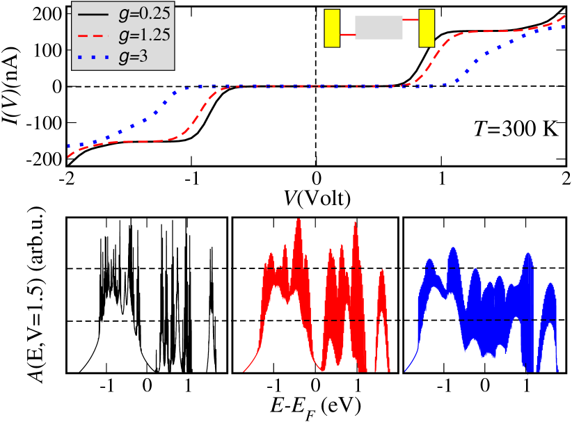
Figure 5: Dependence of the current on the effective electron-vibron coupling strength $g=\lambda/\Omega$ at $T=300$ K and for $t_{X\bar{X}}=0.71\,t$. The vibron frequency was fixed at 20 meV. With increasing coupling the total current is reduced and the zero-current gap is enhanced. The lower panels show the spectral density at $V\sim 1.5\,$Volt for the three values of $g$. Despite the increased number of vibron satellites with increasing coupling, the total intensity is reduced.

Fig. 6 shows in a more systematic way the influence of $\lambda$ and $\Omega$ on the elastic and inelastic components of the total current. The dependence on $\lambda$ is easier to understand since only the prefactors $\phi_{n}(\tau)$ do depend on it. One can show that $\phi_{n=0}(\tau)$ is a monotonous decreasing function of $g$(or $\lambda$), while $\phi_{n\neq 0}(\tau)$ grows up first, reaches a maximum, and then exponentially decays for larger $g$. As a result, the elastic current starts at its bare value for zero coupling to the vibron mode and then it rapidly decreases when increasing the coupling, because the probability for emission/absorption of vibrons accordingly increases. The inelastic component, on the other hand, will first increase for moderate coupling and thus gives the dominant contribution to the total current over some intermediate range of $g$’s (which will also depend on the temperature and the vibron frequency). For even larger $g$’s the inelastic current also goes to zero and the current will be finally suppressed, since there is an increasing trend to charge localization with increasing coupling to the vibron. The behavior at large frequencies is also plausible, see lower panel of Fig. 6, since the average distance between the elastic peak and the inelastic channels is of the order $n\Omega$; if $\Omega$ is large enough an electron injected with a given energy (fixed voltage) will not be able to excite vibrons in the molecular region and thus only the elastic channel will be available. Alternatively, a very stiff mode ($\Omega\to\infty$) will clearly have no influence on the transport. For very low $\Omega$ the inelastic current will obviously vanish, but the elastic component should simply go over into its bare value without charge-vibron coupling. The fact that also the elastic part goes to zero in Fig. 6, lower panel, is simply an artifact related to the fact that at $\Omega=0$ the LF transformation is ill-defined. Since we only consider finite frequencies, this limiting case is not relevant for our discussion.Technical details are presented in Appendix B.

We finally show that extending the previous model to include two vibrational excitations allows for a semi-quantitative description of the experimental results of Ref. [Cohen et al., 2005]. One should, however, keep in mind that these calculations are not giving an explanation of the high currents observed; from the experimental point of view there are some issues like the number of molecules contacted or the specific details of the DNA-metal contacts which are not completely clarified. Our aim is rather to point out at the possible influence of vibrational degrees of freedom in these recent experiments. Using the formalism of Sec. II it is straightforward to obtain expressions for the current in the two-vibron case. One finds ($g_{\rm{s}}=\lambda_{\rm{s}}/\Omega_{s}$, s=1,2):

$$j_{\textrm{tot}}(V) = \frac{e}{2h}\sum^{\infty}_{n=-\infty}\sum^{\infty}_{m=-\infty}\phi_{n,1}\;\phi_{m,2}\int\,dE\,\times$$

$$\{[f_{\textrm{L}}(E)(1-f_{\textrm{R}}(E-(n\Omega_{1}+m\Omega_{2})))$$

$$- f_{\textrm{R}}(E)(1-f_{\textrm{L}}(E-(n\Omega_{1}+m\Omega_{2})))]$$

$$\times t(E-(n\Omega_{1}+m\Omega_{2}))$$

$$+ [f_{\textrm{L}}(E+(n\Omega_{1}+m\Omega_{2}))(1-f_{\textrm{R}}(E))$$

$$- f_{\textrm{R}}(E+(n\Omega_{1}+m\Omega_{2}))(1-f_{\textrm{L}}(E))]$$

$$\times t(E+(n\Omega_{1}+m\Omega_{2}))\}$$

$$\phi_{n,\rm{s}}(\tau) = e^{{-g^{2}_{\rm{s}}(2N_{s}+1)}}\;\times I_{n}(\tau_{s})\;e^{{\beta\Omega_{s}\,n/2}}.$$

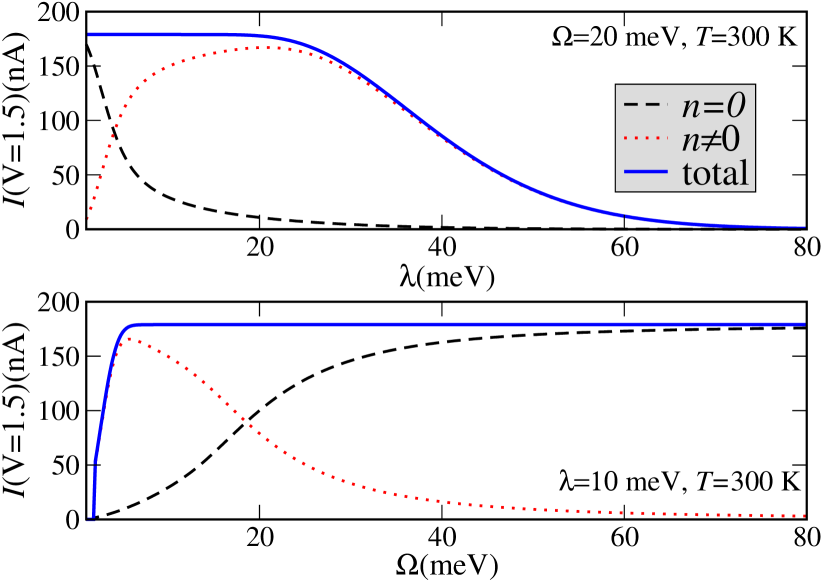
Figure 6: Dependence of the elastic ($n=0$) and inelastic ($n\neq 0$) components of the current at a fixed voltage on the electron-vibron coupling strength $\lambda$ and the mode frequency $\Omega$. A more detailed analysis of the behavior is presented in the text. The dashed lines correspond to the total current (sum of elastic and inelastic components)

The interpretation of the individual contributions is similar to the single-mode case. In Fig. 7 two different experimental curves are shown together with the corresponding theoretical $I$-$V$ plots. Taking into account the simplicity of the model presented in this paper, the agreement is rather good. The values used for the charge-vibron coupling ($\lambda_{1}=15(35)\,\textrm{meV},\lambda_{2}=15(20)\,\textrm{meV}$) and vibron frequencies ($\Omega_{1}=20\,\textrm{meV},\Omega_{2}=6\,\textrm{meV}$) for the yellow (black) theoretical curves have reasonable orders of magnitude for low-frequency modes, see e.g. Ref. [Starikov, 2005]. We stress, however, that the absolute values of the current are mainly determined in our model by the size of the electronic hopping integrals; the influence of the vibrons is to modify the shape and slope of the curves.

To conclude, we have investigated in this paper signatures of electron-vibron interaction in the $I$-$V$ characteristics of a DNA model. Our main motivation were recent experiments on short suspended DNA oligomers with a complex base-pair sequence. Cohen et al. (2005, 2006) The complexity of the physical system under investigation does not allow to draw a definitive conclusion about the mechanism(s) leading to the observed high currents. We have shown that vibrons coupled to the total electronic charge density can considerably influence the current outside the zero-current gap. The “quality” of the molecule-electrode coupling was also shown to modify the orders of magnitude of the current. Another critical parameter in this model, the electronic hopping, may be modified by non-local electron-vibron coupling related, e.g., to inter-base vibrations Berlin et al. (2001); Palmero et al. (2004) or by electron-electron interactions Yi (2003) and as a result, the current profile is also expected to be modify.

Finally we would like to comment on a recent estimation of the maximum current which could be attained in a DNA molecule, which was based on a kinetic model for a molecular wire. Jortner and Bixon (2005) This approach assumes thermal hopping, i.e. sequential tunneling with complete destruction of the phase coherence previous to each hopping process between nearest neighbors. Strikingly, the authors predict a maximum current of the order of pico-Amperes, in contrast to recent experimental results. Xu et al. (2004); Cohen et al. (2005, 2006) As shown in the present paper, the absolute value of the current can be dramatically changed by varying the electronic hopping integrals as well as by the way the two strands are contacted to the electrodes. Moreover, since the electronic matrix elements used in our investigation are on the average larger than the polaron localization energy $\sim g^{2}\Omega$, we are not working in the purely incoherent hopping limit, where the former quantities can be treated as a small perturbation and golden-rule-like expressions do hold. In this respect our model differs from the approach in Ref. [Jortner and Bixon, 2005]. Additional theoretical work is required to bridge kinetic and microscopic model approaches as well as to obtain reliable estimates of the electronic parameters in specific DNA wires including structural fluctuation effects. Voityuk et al. (2001); Senthilkumar et al. (2004) From the experimental point of view it would be highly desirable: (i) to perform a systematic study on the effect of base pair sequence and length dependence on the current and the conductance within the set-up of Ref. [Cohen et al., 2005, 2006], since the length-scaling of the linear conductance is an important benchmark for disclosing the most effective transport channels in molecular wires; (ii) to explore different contact geometries.

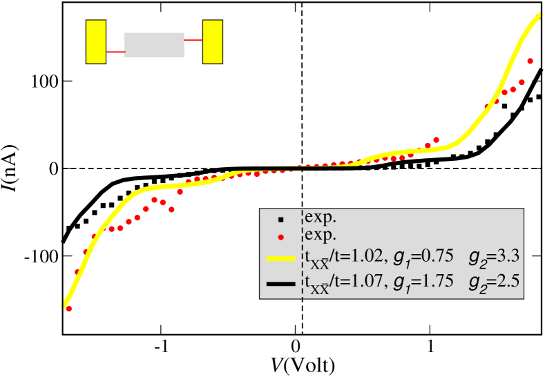
Figure 7: Theoretical curves (solid lines) compared with two different $I$-$V$ curves as obtained on suspended double-strand DNA oligomers contacted by a GNP. Cohen et al. (2005) In both cases the temperature and the coupling to the electrodes were kept fixed at $T=300$ K and $\Gamma_{L,X}=\Gamma_{R,\bar{X}}=250\,\textrm{meV},\Gamma_{R,X}=\Gamma_{L,\bar{X}}=0$, respectively.

V Acknowledgments

We acknowledge fruitful discussions with Igor Brodsky, Joshua Jortner, Ron Naaman, Claude Nogues, and Dmitri Ryndyk. This work has been supported by the Volkswagen Foundation grant Nr. I/78-340, by the EU under contract IST-2001-38951 and by the Israeli Academy of Sciences and Humanities.

Appendix A Derivation of Eq. (8)

In order to derive Eq. 8, all we need to show is that terms proportional to $\textrm{Tr}\{\Gamma_{\textrm{L}}\Gamma_{\textrm{L}}\cdots\}$ and $\textrm{Tr}\{\Gamma_{\textrm{R}}\Gamma_{\textrm{R}}\cdots\}$ identically vanish. Let’s assume e. g. , that $\Gamma_{\textrm{R}}=0$. Thus, the left-going current, which is proportional to $\Gamma_{\textrm{L}}\Gamma_{\textrm{L}}$ must be zero. From Eq. 2, we first obtain:

$$J_{\textrm{L}} = \frac{2\textrm{i}\,e}{h}\sum^{\infty}_{n=-\infty}\phi_{n}(\tau)\,\int dE\;\textrm{Tr}[\Gamma_{\textrm{L}}\{f_{\textrm{L}}(E)G^{>}(E-n\Omega)$$ (10)

$$+ (1-f_{\textrm{L}}(E))G^{<}(E+n\Omega)\}].$$

Use now the kinetic equation for the Green function $G^{<(>)}(E)=G^{r}(E)\Sigma^{<(>)}_{\textrm{L}}(E)G^{a}(E)$, where $\Gamma_{\textrm{R}}=0$ has been already set, and insert it in the above equation with the short-hand notations $C_{\pm}=\textrm{Tr}\{\Gamma_{\textrm{L}}G^{r}(E\pm n\Omega)\Gamma_{\textrm{L}}G^{a}(E\pm n\Omega)\}$. We get:

$$J_{\textrm{L}} = \frac{2e}{h}\sum^{\infty}_{n=-\infty}\phi_{n}(\tau)\,\int dE\{f_{\textrm{L}}(E)\,(1-f_{\textrm{L}}(E-n\Omega))C_{-}$$ (11)

$$- (1-f_{\textrm{L}}(E))\,f_{\textrm{L}}(E+n\Omega)C_{+}\}.$$

If we now change $n\to-n$ in the second term and use the symmetry $\phi_{-n}=\phi_{n}e^{-\beta n\Omega}$ together with the identity $(1-f_{\textrm{L}}(E))=e^{\beta(E-\mu_{\textrm{L}})}f_{\textrm{L}}(E)$, we find:

$$J_{\textrm{L}} = \frac{2e}{h}\sum^{\infty}_{n=-\infty}\phi_{n}(\tau)\,\int dE\,f_{\textrm{L}}(E)\,(1-f_{\textrm{L}}(E-n\Omega))C_{-}$$ (12)

$$\times \{1-e^{\beta(E-\mu_{\textrm{L}})}e^{-\beta(E-\mu_{\textrm{L}}-n\Omega)}e^{-\beta n\Omega}\}=0.$$

This means that only mixed terms containing $\textrm{Tr}\{\Gamma_{\textrm{L}}\cdots\Gamma_{\textrm{R}}\}$ contribute to the current. It is then straightforward to show along the same lines that Eq. 8 comes out.

Appendix B Asymptotic behavior of the current as a function of $\lambda$ and $\Omega$

The asymptotic behavior of the current as a function of the electron-vibron coupling can be immediately understood by looking at the prefactors $\phi_{n}(\tau)$, since only at this place $\lambda$ does appear. Using the asymptotic behavior of the Bessel functions, $I_{n}(z\ll 1)\sim z^{n}/2^{n}n!$ and $I_{n}(z\gg 1)\sim e^{z}/\sqrt{2\pi z}$, one sees that:

$$\phi_{n}(g\ll 1) \sim e^{-g^{2}(2N+1)}\,e^{\beta\Omega n/2}\,\frac{g^{2n}}{n!}[N(N+1)]^{n/2}$$

$$\sim e^{-g^{2}(2N+1)}g^{2n},$$

$$\phi_{n}(g\gg 1) \sim e^{-g^{2}(2N+1)}\,e^{\beta\Omega n/2}\,\frac{e^{2g^{2}Ne^{\beta\Omega/2}}}{\sqrt{4\pi g^{2}Ne^{\beta\Omega/2}}}$$

$$= \frac{e^{\beta\Omega n/2}}{\sqrt{4\pi g^{2}Ne^{\beta\Omega/2}}}\,e^{-g^{2}\,\overbrace{N[e^{\beta\Omega}-2e^{\beta\Omega/2}+1]}^{A>0!}},$$

$$\phi_{n}(g\gg 1) \sim \frac{e^{-g^{2}A}}{g}\to 0.$$

From here it follows that the inelastic current will grow as some power of $g^{2}$ and then decay to zero, while the elastic part ($n=0$) starts from its bare value (at $\lambda=0$) and then rapidly decays for larger values of the electron-vibron interaction.

In order to analyze the behavior of the current for small and large frequencies, it is appropriate to write Eq. 8 in a slightly different form. Doing a change of variables in the $+$ and $-$ components, we arrive at:

$$j_{\textrm{T}} = \phi_{0}(\tau)\,2\frac{e}{h}\,\int dE\,t(E)\,(f_{\textrm{L}}(E)-f_{\textrm{R}}(E))+$$

$$+ \frac{e}{h}\,\sum_{n\neq 0}\phi_{n}(\tau)\,\int dE\,t(E)\,\Lambda_{n}(E,\Omega)$$

$$= j_{\textrm{el}}+j_{\textrm{inel}}$$

$$\Lambda_{n}(E,\Omega) = f_{\textrm{L}}(E+n\Omega)(1-f_{\textrm{R}}(E))-$$

$$- f_{\textrm{R}}(E+n\Omega)(1-f_{\textrm{L}}(E))$$

$$+ f_{\textrm{L}}(E)(1-f_{\textrm{R}}(E-n\Omega))-$$

$$- f_{\textrm{R}}(E)(1-f_{\textrm{L}}(E-n\Omega)).$$

The sum can be now split into terms with $n>0$ and terms with $n<0$. Using the symmetry $\phi_{-n}(\tau)=\phi_{n}(\tau)e^{-\beta\Omega n}$, the above expressions can be cast into the following form:

$$j_{\textrm{T}}=\phi_{0}(\tau)\,2\frac{e}{h}\,\int dE\,t(E)\,(f_{\textrm{L}}(E)-f_{\textrm{R}}(E))+$$

$$+ \frac{e}{h}\,\sum_{n\geq 1}\phi_{n}(\tau)\int dE\,t(E)\left\{\Lambda_{n}(E,\Omega)+\Lambda_{-n}(E,\Omega)e^{-\beta\Omega n}\right\}$$

Let’s consider the case of large vibron frequency. We can use the fact that $f(E\pm n\Omega)$ goes to 0 ($+$) or 1 ($-$) when $\Omega\to\infty$. Note that in this case $\Lambda_{n}(E,\Omega)$ vanishes while $\Lambda_{-n}(E,\Omega)$ goes over into $2(f_{\textrm{L}}(E)-f_{\textrm{R}}(E))$. Using this result together with the asymptotic behavior of the Bessel functions for small arguments leads to:

$$j_{\textrm{inel}} \approx 2\frac{e}{h}\sum_{n\geq 1}\int dE\,t(E)\,(f_{\textrm{L}}(E)-f_{\textrm{R}}(E))\,\times$$

$$\times e^{-g^{2}}\frac{g^{2n}}{n!}\,e^{-\beta\Omega n/2}\,e^{\beta\Omega n/2}e^{-\beta\Omega n}\stackrel{{\scriptstyle\Omega\to\infty}}{{\longrightarrow}}0$$

Hence, the inelastic current vanishes at very large frequencies. The elastic current, however, saturates at the value $(2e/h)\int dE\,t(E)(f_{\textrm{L}}(E)-f_{\textrm{R}}(E))$, since $\phi_{n=0}(\tau)\sim e^{-g^{2}}I_{0}(2g^{2}e^{-\beta\Omega})\to e^{-g^{2}}\to 1$ when $\Omega\to\infty$.

In the case $\Omega\to 0$, the inelastic part of the current will adopt the following form (with $x=\hbar\Omega/k_{\textrm{B}}T)$:

$$j_{\textrm{inel}} \approx 4\frac{e}{h}\sum_{n\geq 1}\int dE\,t(E)\,(f_{\textrm{L}}(E)-f_{\textrm{R}}(E))\,\times$$

$$\times e^{-2g^{2}/x}\frac{e^{2g^{2}/x}}{\sqrt{4\pi g^{2}}}\,\sqrt{x}\,e^{\beta\Omega n}\sim\sqrt{x}\stackrel{{\scriptstyle x\to 0}}{{\longrightarrow}}0,$$

where the asymptotic expansion of the Bessel functions for large argument has been used. A similar scaling would follow for the elastic part of the current, so that for $\Omega\to 0$ the total current is suppressed. This is clearly an artifact of the limiting procedure, since the Lang-Firsov transformation is obviously ill-defined at zero frequency.

References

- Cuniberti et al. (2005) G. Cuniberti, G. Fagas, and K. R. (Eds.), Introducing Molecular Electronics: A brief overview (Springer), Lecture Notes in Physics 680 (2005).
- Keren et al. (2003) K. Keren, R. S. Berman, E. Buchstab, U. Sivan, and E. Braun, Science 302, 1380 (2003).
- Mertig et al. (1999) M. Mertig, R. Kirsch, W. Pompe, and H. Engelhardt, Eur. Phys. J. D 9, 45 (1999).
- Treadway et al. (2002) C. R. Treadway, M. G. Hill, and J. K. Barton, Chem. Phys. 281, 409 (2002).
- Murphy et al. (1993) C. J. Murphy, M. R. Arkin, Y. Jenkins, N. D. Ghatlia, S. H. Bossmann, N. J. Turro, and J. K. Barton, Science 262, 1025 (1993).
- Braun et al. (1998) E. Braun, Y. Eichen, U. Sivan, and G. Ben-Yoseph, Nature 391, 775 (1998).
- Storm et al. (2001) A. J. Storm, J. V. Noort, S. D. Vries, and C. Dekker, Appl. Phys. Lett. 79, 3881 (2001).
- Porath et al. (2000) D. Porath, A. Bezryadin, S. D. Vries, and C. Dekker, Nature 403, 635 (2000).
- Yoo et al. (2001) K.-H. Yoo, D. H. Ha, J.-O. Lee, J. W. Park, J. Kim, J. J. Kim, H.-Y. Lee, T. Kawai, and H. Y. Choi, Phys. Rev. Lett. 87, 198102 (2001).
- Xu et al. (2004) B. Xu, P. Zhang, X. Li, and N. Tao, Nano letters 4, 1105 (2004).
- Cohen et al. (2005) H. Cohen, C. Nogues, R. Naaman, and D. Porath, Proc. Natl. Acad. Sci. USA 102, 11589 (2005).
- Cohen et al. (2006) H. Cohen, C. Nogues, D. Ullien, S. Daube, R. Naaman, and D. Porath, Faraday Discussions 131, 367 (2006).
- Cohen et al. (2004) C. Nogues, H. Cohen, S. Daube, and R. Naaman, Phys. Chem. Chem. Phys. 6, 4459 (2004).
- Artacho et al. (2003) E. Artacho, M. Machado, D. Sanchez-Portal, P. Ordejon, and J. M. Soler, Mol. Phys. 101, 1587 (2003).
- Calzolari et al. (2002) A. Calzolari, R. D. Felice, E. Molinari, and A. Garbesi, Appl. Phys. Lett. 80, 3331 (2002).
- Felice et al. (2004) R. D. Felice, A. Calzolari, and H. Zhang, Nanotechnology 15, 1256 (2004).
- Gervasio et al. (2002) F. L. Gervasio, P. Carloni, and M. Parrinello, Phys. Rev. Lett. 89, 108102 (2002).
- Barnett et al. (2001) R. N. Barnett, C. L. Cleveland, A. Joy, U. Landman, and G. B. Schuster, Science 294, 567 (2001).
- Hübsch et al. (2005) A. Hübsch, R. G. Endres, D. L. Cox, and R. R. P. Singh, Phys. Rev. Lett. 94, 178102 (2005).
- Starikov (2003) E. B. Starikov, Phil. Mag. Lett. 83, 699 (2003).
- Starikov (2005) E. B. Starikov, Phil. Mag. 85, 3435 (2005).
- Adessi et al. (2003) C. Adessi, S. Walch, and M. P. Anantram, Phys. Rev. B 67, 081405(R) (2003).
- Mehrez and Anantram (2005) H. Mehrez and M. P. Anantram, Phys. Rev. B 71, 115405 (2005).
- Cuniberti et al. (2002) G. Cuniberti, L. Craco, D. Porath, and C. Dekker, Phys. Rev. B 65, 241314(R) (2002).
- Jortner et al. (1998) J. Jortner, M. Bixon, T. Langenbacher, and M. Michel-Beyerle, Proc. Natl. Acad. Sci. 95, 12759 (1998).
- Jortner and Bixon (2002) J. Jortner and M. Bixon, Chemical Physics 281, 393 (2002).
- Roche et al. (2003) S. Roche, D. Bicout, E. Macia, and E. Kats, Phys. Rev. Lett. 91, 228101 (2003).
- Roche (2003) S. Roche, Phys. Rev. Lett. 91, 108101 (2003).
- Unge and Stafstrom (2003) M. Unge and S. Stafstrom, Nano letters 3, 1417 (2003).
- Hennig et al. (2004) D. Hennig, E. B. Starikov, J. F. R. Archilla, and F. Palmero, Journal of Biological Physics 30, 227 (2004).
- Jortner and Bixon (2005) J. Jortner and M. Bixon, Chem. Phys. 319, 273 (2005).
- Apalkov and Chakraborty (2005a) V. M. Apalkov and T. Chakraborty, Phys. Rev. B 71, 033102 (2005a).
- Apalkov and Chakraborty (2005b) V. Apalkov and T. Chakraborty, Phys. Rev. B 72, 161102(R) (2005b).
- Gutierrez et al. (2005a) R. Gutierrez, S. Mandal, and G. Cuniberti, Nano letters 5, 1093 (2005a).
- Gutierrez et al. (2005b) R. Gutierrez, S. Mandal, and G. Cuniberti, Phys. Rev. B 71, 235116 (2005b).
- Kohler et al. (2005) S. Kohler, J. Lehmann, and P. Hänggi, Phys. Rep. 406, 379 (2005).
- Yamada et al. (2004) H. Yamada, E. B. Starikov, D. Hennig, and J. F. R. Archilla, Eur. Phys. J. E 17, 149 (2005).
- D’Orsogna and Bruinsma (2003) M. R. D’Orsogna and R. Bruinsma, Phys. Rev. Lett. 90, 078301 (2003).
- Koch and von Oppen (2005) J. Koch and F. von Oppen, Phys. Rev. Lett. 94, 206804 (2005).
- de Pablo et al. (2000) P. J. dePablo, J. Colchero, M. Luna, J. Gomez-Herrero, and A. M. Baro, Phys. Rev. B 61, 14179 (2000).
- Yi (2003) J. Yi, Phys. Rev. B 68, 193103 (2003).
- Yamada (2004) H. Yamada, Phys. Lett. A 332, 65 (2004).
- Klotsa et al. (2005) D. Klotsa, R. A. Roemer, and M. S. Turner, Biophys. J. 89, 2187 (2005).
- Caetano and Schulz (2005) R. A. Caetano and P. A. Schulz, Phys. Rev. Lett. 95, 126601 (2005).
- Wang and Chakraborty (2006) X. F. Wang and T. Chakraborty, cond-mat/0603672 (2006).
- Voityuk et al. (2000) A. Voityuk, N. Rösch, M. Bixon, and J. Jortner, J. Phys. Chem. B 104, 5661 (2000).
- Voityuk et al. (2001) A. Voityuk, K. Siriwong, and N. Rösch, Phys. Chem. Chem. Phys 3, 5421 (2001).
- Grozema et al. (2002) F. C. Grozema, L. D. A. Siebbeles, Y. A. Berlin,and M. A. Ratner, ChemPhysChem 6, 536 (2002).
- Berlin et al. (2001) Y. A. Berlin, A. L. Burin, and M. A. Ratner, J. Am. Chem. Soc. 123, 260 (2001).
- Grozema et al. (2001) F. C. Grozema, Y. A. Berlin, and L. D. A. Siebbeles, J. Am. Chem. Soc. 122, 10903 (2000).
- Palmero et al. (2004) F. Palmero, J. F. R. Archilla, D. Hennig, and F. R. Romero, New J. Phys. 6, 13 (2004).
- Senthilkumar et al. (2004) K. Senthilkumar, F. C. Grozema, C. Fonseca, F. M. Bickelhaupt, F. D. Lewis, Y. A. Berlin, M. A. Ratner, and L. D. A. Siebbeles, J. Am. Chem. Soc. 127, 14894 (2005).
- Mahan (2000) G. D. Mahan, Many-Particle Physics (Plenum Press, New York, 2000), 3rd ed.
- Hewson and Newns (1979) A. C. Hewson and D. M. Newns, J. Phys. C: Solid State Phys. 12, 1665 (1979).
- Meir and Wingreen (1992) Y. Meir and N. S. Wingreen, Phys. Rev. Lett. 68, 2512 (1992).
- Felice et al. (2002) R. Di Felice, A. Calzolari, E. Molinari, and A. Garbesi, Phys. Rev. B 65, 045104 (2002).
- Tran et al. (2000) P. Tran, B. Alavi, and G. Gruner, Phys. Rev. Lett. 85, 1564 (2000).
- Rakitin et al. (2001) A. Rakitin, P. Aich, C. Papadopoulos, Y. Kobzar, A. S Vedeneev, J. S.. Lee, and J. M. Xu, Phys. Rev. Lett. 86, 3670 (2001).
- Zalinge et al. (2006) H. van Zalinge, D. J. Schiffrin, A. D. Bates, W. Haiss, J. Ulstrup, and R. J. Nichols, ChemPhysChem 7, 94 (2006).