Effects of mixing and stirring on the critical behaviour

Abstract

Stochastic dynamics of a nonconserved scalar order parameter near its critical point, subject to random stirring and mixing, is studied using the field theoretic renormalization group. The stirring and mixing are modelled by a random external Gaussian noise with the correlation function $\propto\delta(t-t^{\prime})k^{4-d-y}$ and the divergence-free (due to incompressibility) velocity field, governed by the stochastic Navier–Stokes equation with a random Gaussian force with the correlation function $\propto\delta(t-t^{\prime})k^{4-d-y^{\prime}}$. Depending on the relations between the exponents $y$ and $y^{\prime}$ and the space dimensionality $d$, the model reveals several types of scaling regimes. Some of them are well known (model A of equilibrium critical dynamics and linear passive scalar field advected by a random turbulent flow), but there are three new nonequilibrium regimes (universality classes) associated with new nontrivial fixed points of the renormalization group equations. The corresponding critical dimensions are calculated in the two-loop approximation (second order of the triple expansion in $y$, $y^{\prime}$ and $\varepsilon=4-d$).

1 Introduction

Over the past three decades, increasing attention has been attracted by the dynamics of phase ordering — the growth of order through domain coarsening (spinodal decomposition), when a system (e.g. a ferromagnet or a binary alloy) is quenched from its high-temperature homogeneous phase into the low-temperature multi-phase coexistence region; see [1]–[18] and references therein.

Much interest was focused on the late stages of the coarsening process, when some kind of a self-similar (scaling) regime develops with apparently universal exponents — the features normally associated with the critical behaviour. That regime is by now rather well understood; see Ref. [1] and the reviews cited the. Phenomenological approaches, renormalization group (RG) techniques, exactly soluble models and numerical simulations show that the characteristic domain size increases as a power of time, $L(t)\sim t^{\alpha}$, where the growth exponent $\alpha$ depends on the global characteristics of the system (conserving or nonconserving dynamics, scalar or vector order parameter, dimensionality of space) but not on its detailed structure (like the values of the coupling constants). Therefore, in recent years attention has been directed to systems subjected to external stirring, like binary mixtures under imposed shear flow or other kinds of deterministic or random (e.g. turbulent) velocity fields; see [3]–[15] and references therein.

Numerical experiments and theoretical analysis (e.g. the linear stability analysis of the corresponding dynamic equations) of binary alloys subjected to statistically isotropic and homogeneous random velocity ensembles of very different kinds also suggest that, at least close to the critical point and under vigorous stirring, the domain growth is “arrested” and a new dynamical nonequilibrium steady state emerges, which is characterized by a continuous formation and rupture of finite-size domains [3, 9, 16, 18].

Emergence of the nonequilibrium steady states appears rather a generic and robust phenomenon, being observed in two-dimensional numerical simulations for passive [9, 16, 18] and active [18] order parameters subjected to a random Gaussian velocity field with finite correlation length and time [9] and various kinds of regular and chaotic cellular flows [16, 18]. The questions which naturally arise within this context, and which will be addressed in the present paper, are the following: Do those steady states reveal some kinds of self-similar behaviour? Do the corresponding correlation and structure functions exhibit power laws? If yes, do those states belong to the universality classes known for the models of equilibrium critical dynamics [19, 20], or do they represent new types of scaling behaviour? Are there any crossover dimensions for the new scaling regimes? Is it possible to establish the existence of these scaling regimes on the basis of microscopic models, and to calculate the corresponding exponents in consistent approximations or, better, within regular perturbation expansions? To what extent this behaviour is universal? What are the parameters the scaling dimensions depend on?

We will consider the dynamics of a scalar (one-component) passive (no feedback on the velocity field) nonconserving order parameter $\varphi(x)\equiv\varphi(t,{\bf x})$ governed by the stochastic equation

$$\sigma_{0}\nabla_{t}\varphi=\partial^{2}\varphi-V^{\prime}(\varphi)+f,\qquad\nabla_{t}=\partial_{t}+v_{i}\partial_{i},$$ (1)

where $\sigma_{0}>0$ is the reciprocal of the kinetic coefficient and the potential $V(\varphi)$ will be chosen as in the well-known models of critical dynamics [19, 20, 21, 22]. However, in contrast to the latter, the stirring noise $f(x)$ and the velocity $v_{i}(x)$ are not chosen such that the steady state of the system is in equilibrium, or, in other words, its equal-time correlation functions are not described by the Landau–Ginzburg Hamiltonian. Namely, the transverse (divergence-free, due to the incompressibility condition $\partial_{i}v_{i}=0$) velocity field satisfies the Navier–Stokes equation with a random driving force

$$\nabla_{t}v_{i}=\nu_{0}\partial^{2}v_{i}-\partial_{i}{\cal P}+f_{i},$$ (2)

where ${\cal P}$ and $f_{i}$ are the pressure and the transverse random force per unit mass (all these quantities depend on $x$).

The random sources $f(x)$ and $f_{i}(x)$ maintain the steady state of the system and model the effects of external stirring and/or shaking and initial and/or boundary conditions. The use of such random stirring terms is a commonplace in the statistical theory of turbulence [23, 24, 25, 26] and other nonequilibrium phenomena [23, 27]: it allows one to do away with the details of the geometry of the system and to consider a homogeneous and isotropic problem in the infinite space. Let us specify their statistical properties.

In models of equilibrium critical dynamics the form of such correlators for Langevin equations (like e.g. (2) without the velocity) is uniquely determined by the requirement that the dynamics and statics be mutually consistent (that is, the equal-time correlations of the dynamical problem be given by the Landau–Ginzburg Hamiltonian); see [19, 20, 21]. Such arguments do not apply to our non-equilibrium model. Like in the RG theory of turbulence, the correlators will be chosen on the basis of both physical and technical arguments.

Consider for definiteness the correlation function

$$D_{\varphi}(x,x^{\prime})\equiv\langle f(x)f(x^{\prime})\rangle=\delta(t-t^{\prime})\,D(r),\qquad r=|{\bf x}-{\bf x}^{\prime}|,$$ (3)

of the source field of the stochastic equation (1). The function $D(r)$ depends only on $r=|{\bf x}-{\bf x}^{\prime}|$, its Fourier transform being $D(k)$. The physical arguments are that the noises model the injection of energy to the system owing to interaction with the large-scale stirring. Thus for realistic case the dominant contribution to the correlators $D(k)$ must come from small momenta $k\sim m$, where $m=1/L$ is the reciprocal of the integral (external) scale $L$ (the size of the system or a stirring device). Idealized injection by infinitely large modes corresponds to $D(k)\propto\delta({\bf k})$. On the other hand, for the use of the standard RG technique it is important that the function $D(k)$ have a power-law behaviour at large $k$. This condition is satisfied if $D(k)$ is chosen in the form [24] $D(k)=D_{0}\,h(m/k)\,k^{4-d-y}$, where $D_{0}>0$ is an amplitude factor, $d$ is the space dimension and the exponent $y$ plays the part analogous to that played by $4-d$ in the RG theory of critical behaviour. The function $h(m/k)$ with $h(0)=1$ provides the IR regularization. Its specific form is unessential; we will use the sharp cutoff $h(m/k)=\theta(m-k)$ with the Heaviside step function to simplify the practical calculation (in the calculations in the spirit of dimensional regularization one could simply set $h=1$).

The large-scale forcing is reproduced in the limit $y\to 4$, as follows from the well-known power-law representation of the $d$-dimensional $\delta$ function,

$$\delta({\bf k}) = \lim_{y\to 4}\,\frac{1}{(2\pi)^{d}}\int d{\bf x}\,(\Lambda x)^{y-4}\,\exp[{\rm i}({\bf k}\cdot{\bf x})]=$$ (4)

$$= S_{d}^{-1}k^{-d}\lim_{y\to 4}\left[(4-y)(k/\Lambda)^{4-y}\right],$$

where $S_{d}$ is the surface area of the unit sphere in $d$-dimensional space (see (17ao) in section 6) and $\Lambda$ has the dimension of a momentum. Representation (4) also specifies the appropriate choice of the amplitude $D_{0}$ at $y\to 4$. More detailed discussion of this issue can be found in section 6.3 of book [21].

Following these ideas, the sources $f(x)$ and $f_{i}(x)$ will be taken Gaussian, white in time (this is dictated by the principle of maximum entropy [28]) and with power-law spectra, $\langle ff\rangle\propto\delta(t-t^{\prime})k^{4-d-y}$ for the scalar noise and $\langle f_{i}f_{j}\rangle\propto\delta(t-t^{\prime})P_{ij}({\bf k})k^{4-d-y^{\prime}}$ for the vector one, where ${\bf k}$ is the momentum (wave vector), $k=|{\bf k}|$ is the wave number, $d$ is the space dimensionality, $P_{ij}({\bf k})=\delta_{ij}-k_{i}k_{j}/k^{2}$ is the transverse projector, and $y$ and $y^{\prime}$ are arbitrary parameters. The large-scale forcing corresponds to the limits $y$, $y^{\prime}\to 4$.

The time decorrelation of the random force guarantees that the full stochastic problem (1), (2) is Galilean invariant for all values of the model parameters, including $D_{0}$ and $d$. As a consequence, the ordinary perturbation theory for the model (the expansion in the nonlinearities) is manifestly Galilean covariant: all the exact relations between the correlation functions imposed by the Galilean symmetry (Ward identities) are satisfied order by order. The renormalization procedure does not violate the Galilean symmetry, so that the improved perturbation expansion, obtained with the aid of RG, also remains covariant.

In a wider context, the model (1), (2) can be interesting as a model system for studying generic nonequilibrium dynamical features. Recently, significant progress has been achieved in classifying large-scale, long-distance scaling behaviour of such phenomena, including driven diffusive systems, diffusion-limited reactions, growth, ageing and percolation processes, and so on; see e.g. [29] and references therein. Being analytically tractable, our model can serve as a good testing ground in studying such scaling regimes and their universality. Similar (but nonstationary) models also arise in stochastic inflationary models designed to describe the structure formation in cosmology; see [30].

We will apply to the stochastic problem (1) the field theoretic renormalization group (RG), which proved to be extremely useful in describing equilibrium critical phenomena, including their kinetic properties [19, 20, 21, 22]. In the RG framework, long-wavelength scaling regimes are associated with infrared (IR) attractive fixed points of the corresponding RG equations. Earlier, the RG approach was applied to the problem of phase separation and domain growth in a number of studies [1, 5, 6, 7, 8]. By contrast with critical phenomena, however, the application of the RG to the growth problems suffers from the lack of an (obvious) small parameter (analogous to $\varepsilon=4-d$ for the Landau–Ginzburg model and corresponding dynamical models), the problem also encountered for the stochastic Burgers and Kardar–Parisi–Zhang models [23, 27]. To circumvent this obstacle, in [1, 5, 6, 7, 8], the RG was used in the form of block-spin transformations performed using numerical Monte Carlo simulations, proposed earlier in [31]. Another possibility, explored in [8] (see also discussion in the review paper [1]), was to assume the existence of the RG symmetry and an appropriate strong-coupling fixed point, and then to use specific features of the conserved dynamics (absence of renormalization of the transport coefficient, well known for the model B of equilibrium dynamics [19, 20, 21]) to derive some exact relations between the critical exponents. To complete that analysis, however, one should take some exponents from the experiment or derive them using additional phenomenological considerations [1, 8].

The plan of the paper is as follows. We begin with the analysis of the model without velocity, which appears nontrivial and reveals a new type of scaling behaviour. In section 2 we present the field theoretic formulation of the model and its renormalization. After an appropriate extension, the model becomes multiplicatively renormalizable, and the differential RG equations can be derived in a standard fashion (section 3). The fixed points and their regions of IR stability are analyzed in section 4. It is shown that a systematic perturbation expansion in the two parameters, $y$ and $\varepsilon=4-d$, can be constructed for the coordinates of the fixed points and critical dimensions, with the additional assumption that $y-\varepsilon=O(\varepsilon^{2})$. One of the two nontrivial fixed points corresponds to the well known model A of equilibrium critical dynamics, while the other represents a new nonequilibrium universality class; the corresponding critical dimensions are calculated in the two-loop approximation (section 5). In section 6, the full model with the velocity field, governed by the stochastic Navier–Stokes equation, is studied. Two additional nonequilibrium scaling regimes (universality classes) are identified; the corresponding dimensions are found to the second order of the triple expansion in $y$, $y^{\prime}$ and $\varepsilon=4-d$. Section 7 is reserved for a brief conclusion. Some interesting details of the two-loop calculation are given in A.

The field-theoretic renormalization group was earlier applied to the problem of the effects of turbulence on the critical behaviour of binary mixtures in [17]. The model studied in that work was less realistic than the present one in two respects: turbulence was modelled by a Gaussian time-decorrelated statistical ensemble and the noise was taken to be purely thermal. On the other hand, our model is less realistic in the sense that the order parameter here is not conserved. Nevertheless, the main qualitative conclusion drawn from the two cases is the same: the instability of the equilibrium fixed point and the existence of a new non-equilibrium critical regime was established. Thus we may conclude that such a phenomenon appears quite robust and insensitive to the details of the model.

2 The model without convection: Field theoretic formulation and renormalization

It is instructive to begin the analysis with the model with no convection term in (1), which already exhibits a nonequilibrium scaling regime and involves some interesting formal subtleties. The dynamical equation for the order parameter $\varphi(x)\equiv\varphi(t,{\bf x})$ then becomes

$$\sigma_{0}\partial_{t}\varphi=\partial^{2}\varphi-V^{\prime}(\varphi)+f.$$ (5)

Correlator of the random noise $f(x)$ will be taken in the form

$$D_{\varphi}(x,x^{\prime})\equiv\langle f(x)f(x^{\prime})\rangle=\delta(t-t^{\prime})\,D(r),\qquad r=|{\bf x}-{\bf x}^{\prime}|,$$ (6)

with some function $D(r)$ depending only on $r=|{\bf x}-{\bf x}^{\prime}|$. The choice $D(r)=2\sigma_{0}\delta({\bf x}-{\bf x}^{\prime})$ corresponds to the well-known model A of critical dynamics, which describes kinetic properties of the equilibrium critical state [19, 20, 21, 22]; the probability distribution function of its equal-time correlators is then given by $\exp\left(-H(\varphi)\right)$ where $H(\varphi)=-\varphi\partial^{2}\varphi+V(\varphi)$ with the implied integration over ${\bf x}$ is the Hamiltonian for the time-independent field $\varphi({\bf x})$.

We assume that the model is near its critical point, and, in the spirit of the Landau theory, retain in $V(\varphi)$ only the first terms of the Taylor expansion: $V(\varphi)=\tau_{0}\varphi^{2}/2+\lambda_{0}\varphi^{4}/24$, where $\tau_{0}$ is the deviation of the temperature from its critical value. The function $D(r)$ in (6), however, will be chosen in the power-like form $D(r)\propto r^{-4+y}$, which in the momentum representation gives

$$D(k)=D_{0}k^{4-d-y},$$ (7)

where $k=|{\bf k}|$ is the wave number, $y$ is an arbitrary parameter and $D_{0}>0$ an amplitude factor. The IR cutoff at $k=m$ is implied.

According to the general theorem (see e.g. [21, 22]), stochastic problem (5), (6) is equivalent to the field theoretic model of the doubled set of fields $\Phi\equiv\{\varphi^{\prime},\varphi\}$ with action functional

$$S(\Phi)=\varphi^{\prime}D_{\varphi}\varphi^{\prime}/2+\varphi^{\prime}\left\{-\sigma_{0}\partial_{t}\varphi+\partial^{2}\varphi-\tau_{0}\varphi-\lambda_{0}\varphi^{3}/6\right\},$$ (8)

with $D_{\varphi}$ from (6) and implied integrations over the argument $x=\{t,{\bf x}\}$. Formulation (8) means that statistical averages of random quantities in the original stochastic problem can be represented as functional averages with the weight $\exp S(\Phi)$. The model (8) corresponds to a standard Feynman diagrammatic technique with two bare propagators (lines in the diagrams) $\langle\varphi\varphi\rangle_{0}$ and $\langle\varphi\varphi^{\prime}\rangle_{0}$ (their explicit form is given in A) and the vertex $\varphi^{\prime}\varphi^{3}$.

The analysis of ultraviolet (UV) divergences is based on the analysis of canonical dimensions. Dynamical models of the type (8), in contrast to static models, have two scales, i.e., the canonical dimension of some quantity $F$ (a field or a parameter in the action functional) is described by two numbers, the momentum dimension $d_{F}^{k}$ and the frequency dimension $d_{F}^{\omega}$. They are determined such that $[F]\sim[L]^{-d_{F}^{k}}[T]^{-d_{F}^{\omega}}$, where $L$ is the length scale and $T$ is the time scale. The dimensions are found from the obvious normalization conditions $d_{k}^{k}=-d_{\bf x}^{k}=1$, $d_{k}^{\omega}=d_{\bf x}^{\omega}=0$, $d_{\omega}^{k}=d_{t}^{k}=0$, $d_{\omega}^{\omega}=-d_{t}^{\omega}=1$, and from the requirement that each term of the action functional be dimensionless (with respect to the momentum and frequency dimensions separately). Then, based on $d_{F}^{k}$ and $d_{F}^{\omega}$, one can introduce the total canonical dimension $d_{F}=d_{F}^{k}+2d_{F}^{\omega}$ (in the free theory, $\partial_{t}\propto\partial^{2}$), which plays in the theory of renormalization of dynamical models the same role as the conventional (momentum) dimension does in static problems, see e.g. [21]. The resulting canonical dimensions are given in table 1, including the dimensions of the parameters which will appear later on (renormalized parameters and the others). It is easily checked that the role of the coupling constant (expansion parameter in the ordinary perturbation theory) in model (8) with correlator (6) is played by the combination $\lambda_{0}D_{0}/\sigma_{0}$. From table 1 it follows that this constant has the dimension $\Lambda^{y}$ with some momentum scale $\Lambda$. Thus the case $y<0$ corresponds to the Gaussian IR behaviour (perturbation theory works in the IR range), $y=0$ is the logarithmic value, and for $y\geq 0$ the RG summation is needed. The UV divergences have the form of the poles in $y$ in the correlation functions of the fields $\Phi\equiv\{\varphi^{\prime},\varphi\}$.

The total canonical dimension of an arbitrary 1-irreducible correlation function $\Gamma=\langle\Phi\cdots\Phi\rangle$ is given by the relation $d_{\Gamma}=d_{\Gamma}^{k}+2d_{\Gamma}^{\omega}=d+2-N_{\Phi}d_{\Phi}$, where $N_{\Phi}=\{N_{\varphi},N_{\varphi^{\prime}}\}$ are the numbers of corresponding fields entering into the function $\Gamma$, and the summation over all types of the fields is implied. The total dimension $d_{\Gamma}$ in the logarithmic theory (that is, at $y=0$) is the formal index of the UV divergence. Superficial UV divergences, whose removal requires counterterms, can be present only in those functions $\Gamma$ for which $d_{\Gamma}$ is a non-negative integer. Straightforward analysis shows that for all $d>4$, superficial UV divergences can be present only in the 1-irreducible functions $\langle\varphi^{\prime}\varphi\rangle$ with the counterterms $\varphi^{\prime}\partial_{t}\varphi$, $\varphi^{\prime}\partial^{2}\varphi$, $\tau_{0}\varphi^{\prime}\varphi$, and $\langle\varphi^{\prime}\varphi^{3}\rangle$ with the counterterm $\varphi^{\prime}\varphi^{3}$. Such terms are present in the action (8), so that the model is multiplicatively renormalizable.

However, for $d\leq 4$ a new divergence appears in the function $\langle\varphi^{\prime}\varphi^{\prime}\rangle$ (for $d=4$ and small $y$, the noise correlator becomes almost polynomial in ${\bf k}$ — namely constant — and local in ${\bf x}$ representation). It would be erroneous to try to eliminate this divergence by renormalizing the nonlocal noise term (as thoroughly discussed in Ref. [32] for the stochastic Navier–Stokes equation). We therefore must add the local counterterm of the form $\varphi^{\prime}\varphi^{\prime}$. So we are forced to consider the variable space dimension and, for $d\leq 4$, to extend the original model (to include the local term in the noise correlator from the very beginning) in order to have multiplicative renormalizability. Finally we arrive at the extended model

$$\sigma_{0}\partial_{t}\varphi=\partial^{2}\varphi-\tau_{0}\varphi-\lambda_{0}\varphi^{3}/6+f,$$ (9)

$$\langle f(x)f(x^{\prime})\rangle=2\sigma_{0}\,\delta(t-t^{\prime})\left\{w_{0}\,k^{4-d-y}+1\right\}$$ (10)

which has become multiplicatively renormalizable for $d<4$; the special case $w_{0}=0$ gives the model A (which is multiplicatively renormalizable in itself). Interpretation of the additional local term in (10) can be twofold. On the one hand, the fact that it is generated by the renormalization procedure means that it is not forbidden by dimensionality or symmetry considerations and, therefore, it is natural to include it in the model from the very beginning. In the language of the Wilsonian RG, this means that such term necessarily arises in the effective model for the properly smoothed (coarse-grained) field; it becomes IR relevant for $d<4$, where it affects the critical behaviour and cannot be neglected. On the other hand, one can insist on studying the original model with a purely power-law correlation function. Then the extension of the model is only needed to ensure the multiplicative renormalizability and to derive the RG equations; the latter should be solved with the special initial data that correspond to the power-law correlator. Since the IR attractive fixed point of the RG equations is unique for any given choice of the parameters $\varepsilon$ and $y$ (see section 4), the resulting IR behaviour is the same as for the case of the general correlation function (10) with the inclusion of the local term.

By dimension the couplings $\lambda_{0}\sim\Lambda^{\varepsilon}$ and $w_{0}\sim\Lambda^{y-\varepsilon}$ with $\varepsilon=4-d$, so that we expect the double RG expansion in $y$ in $\varepsilon$ instead of a single expansion in $y$ (as for $d>4$) or in $\varepsilon$ (as for the model A). However, as we will see, the real situation appears slightly more complicated.

The renormalized action is

$$S_{R}(\varphi,\varphi^{\prime})=\sigma\varphi^{\prime}\left\{w\mu^{y-\varepsilon}k^{\varepsilon-y}+Z_{1}\right\}\varphi^{\prime}$$

$$+\varphi^{\prime}\left\{-Z_{2}\sigma\partial_{t}\varphi+Z_{3}\partial^{2}\varphi-\tau Z_{5}\varphi-Z_{4}\lambda\mu^{\varepsilon}\varphi^{3}/6\right\},$$ (11)

which is equivalent to the multiplicative renormalization of the fields $\varphi\to Z_{\varphi}\varphi$, $\varphi^{\prime}\to Z_{\varphi}^{\prime}\varphi^{\prime}$ and parameters

$$\sigma_{0}=Z_{\sigma}\sigma,\quad\tau_{0}=Z_{\tau}\tau,\quad u_{0}=\mu^{\varepsilon}Z_{u}u,\quad w_{0}=\mu^{y-\varepsilon}Z_{w}w,$$ (12)

where we introduced the new coupling constant $u=\lambda/16\pi^{2}$ (the coefficients in RG functions become slightly simpler) and $\mu$ is the reference mass – additional parameter of the renormalized theory.

The renormalization constants $Z_{i}=Z_{i}(\varepsilon,y,g,w)$ capture the divergences at $\varepsilon,y\to 0$, so that the correlation functions of the renormalized model (11) have finite limits for $\varepsilon,y=0$ (when expressed in renormalized parameters $u$, $w$, $\tau$ and $\mu$).

The relations between the $Z$’s in (11) and (12) have the forms

$$Z_{\sigma}Z_{\varphi^{\prime}}^{2}=Z_{1},\quad Z_{\sigma}Z_{\varphi^{\prime}}^{2}Z_{w}=1,\quad Z_{\sigma}Z_{\varphi^{\prime}}Z_{\varphi}=Z_{2},$$

$$Z_{\varphi}Z_{\varphi^{\prime}}=Z_{3},\quad Z_{\tau}Z_{\varphi}Z_{\varphi^{\prime}}=Z_{5},\quad Z_{u}Z_{\varphi}^{3}Z_{\varphi^{\prime}}=Z_{4}.$$ (13)

The renormalization constants $Z_{1}$–$Z_{5}$ are calculated according to standard rules from the perturbation theory; then the constants in (12) are easily found using the relations (13). The expansion parameter in the $Z$’s is $u$, while the dependence on the second coupling constant $w$ should be calculated exactly in each order of the expansion in $u$. Like for the model A, the first nontrivial contributions to the constants $Z_{4,5}$ are determined by one-loop Feynman graphs, so that $Z_{4,5}=1+O(u)$. The leading contributions to the constants $Z_{1}$–$Z_{3}$ are determined by two-loop (“watermelon”) graphs depicted in figure 1, so that $Z_{1,2,3}=1+O(u^{2})$. These details will be important in the analysis of the fixed points of the RG equations. The two-loop calculation of the renormalization constants in our model is illustrated by the example of $Z_{1}$ in A.

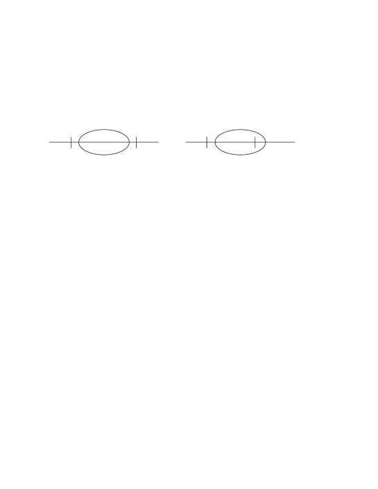
Figure 1: Two-loop graphs giving rise to renormalization constants $Z_{1}$–$Z_{3}$. The simple lines correspond to the bare propagator $\langle\varphi\varphi\rangle_{0}=2\sigma\,\left\{w\,(k/\mu)^{y-\varepsilon}+1\right\}/(\omega^{2}\sigma^{2}+k^{4})$ in frequency-momentum representation, whereas the lines with a slash to the propagator $\langle\varphi\varphi^{\prime}\rangle_{0}=(-{\rm i}\sigma\omega+k^{2})^{-1}$, the slash indicating the variables of the the field $\varphi^{\prime}$. The vertex factor is $\lambda\mu^{\varepsilon}$.

3 RG equations and RG functions

Let us recall an elementary derivation of the RG equations; see [21]. The RG equations are written for the renormalized correlation functions $G_{R}=\langle\Phi\cdots\Phi\rangle_{R}$, which differ from the original (unrenormalized) ones $G=\langle\Phi\cdots\Phi\rangle$ only by normalization and choice of parameters, and therefore can be equally used for analyzing the critical behaviour. The relation $S_{R}(\Phi,e,\mu)=S(\Phi,e_{0})$ between the functionals (8) and (11) results in the relations $G(e_{0},\dots)=Z_{\varphi}^{N_{\varphi}}Z_{\varphi^{\prime}}^{N_{\varphi^{\prime}}}G_{R}(e,\mu,\dots)$ between the correlation functions. Here, as usual, $N_{\varphi}$ and $N_{\varphi^{\prime}}$ are the numbers of corresponding fields entering into $\Gamma$; $e_{0}=\{\sigma_{0},\tau_{0},w_{0},\lambda_{0}\}$ is the full set of bare parameters and $e=\{\sigma,\tau,w,\lambda\propto u\}$ are their renormalized analogs; the dots stand for the other arguments (times, coordinates, momenta etc). We use $\widetilde{\cal D}_{\mu}$ to denote the differential operation $\mu\partial_{\mu}$ for fixed $e_{0}$ and operate on both sides of this equation with it. This gives the basic RG differential equation:

$$\left\{{\cal D}_{RG}+N_{\varphi}\gamma_{\varphi}+N_{\varphi^{\prime}}\gamma_{\varphi^{\prime}}\right\}\,G^{R}(e,\mu,\dots)=0,$$ (14)

where ${\cal D}_{RG}$ is the operation $\widetilde{\cal D}_{\mu}$ expressed in the renormalized variables:

$${\cal D}_{RG}\equiv{\cal D}_{\mu}+\beta_{u}\partial_{u}+\beta_{w}\partial_{w}-\gamma_{\sigma}{\cal D}_{\sigma}-\gamma_{\tau}{\cal D}_{\tau}.$$ (15)

In equation (15), we have written ${\cal D}_{x}\equiv x\partial_{x}$ for any variable $x$, the RG anomalous dimensions $\gamma$ are defined as

$$\gamma_{F}\equiv\widetilde{\cal D}_{\mu}\ln Z_{F}\quad{\rm for\ any\ quantity}\ F,$$ (16)

and the $\beta$ functions for the two dimensionless couplings $u$ and $w$ are

$$\beta_{u}\equiv\tilde{\cal D}_{\mu}u = u[-\varepsilon-\gamma_{u}],$$ (17a)

$$\beta_{w}\equiv\tilde{\cal D}_{\mu}w = w[-y+\varepsilon-\gamma_{w}],$$ (17b)

where the last equalities come from the definitions and relations (12).

The anomalous dimensions $\gamma_{1}$–$\gamma_{5}$ are found from the known constants $Z_{1}$–$Z_{5}$ (see A for $\gamma_{1}$). Then the relations (13) give

$$\gamma_{\sigma}+2\gamma_{\varphi^{\prime}}=\gamma_{1},\quad\gamma_{\sigma}+2\gamma_{\varphi^{\prime}}+\gamma_{w}=0,\quad\gamma_{\sigma}+\gamma_{\varphi^{\prime}}+\gamma_{\varphi}=\gamma_{2},$$

$$\gamma_{\varphi}+\gamma_{\varphi^{\prime}}=\gamma_{3},\quad\gamma_{\tau}+\gamma_{\varphi}+\gamma_{\varphi^{\prime}}=\gamma_{5},\quad\gamma_{u}+3\gamma_{\varphi}+\gamma_{\varphi^{\prime}}=\gamma_{4}.$$ (17r)

Resolving these relations gives

$$\gamma_{\sigma}=\gamma_{2}-\gamma_{3},\quad\gamma_{\tau}=\gamma_{5}-\gamma_{3},\quad\gamma_{u}=\gamma_{1}-\gamma_{2}-2\gamma_{3}+\gamma_{4},$$

$$\gamma_{w}=-\gamma_{1},\quad 2\gamma_{\varphi}=\gamma_{3}+\gamma_{2}-\gamma_{1},\quad 2\gamma_{\varphi^{\prime}}=\gamma_{1}+\gamma_{3}-\gamma_{2},$$ (17s)

and for the $\beta$ functions (16) one obtains:

$$\beta_{u}=u[-\varepsilon-\gamma_{1}+\gamma_{2}+2\gamma_{3}-\gamma_{4}],\qquad\beta_{w}=w[-y+\varepsilon+\gamma_{1}].$$ (17t)

4 Fixed points and scaling regimes

It is well known that possible scaling regimes of a renormalizable model are associated with the IR attractive fixed points of the corresponding RG equations. In our model, the coordinates $u_{*}$, $w_{*}$ of the fixed points are found from the equations

$$\beta_{u}(u_{*},w_{*})=0,\quad\beta_{w}(u_{*},w_{*})=0$$ (17u)

with the beta functions given in (17t). The type of a fixed point is determined by the matrix $\Omega=\{\Omega_{ij}=\partial\beta_{i}/\partial g_{j}\}$, where $\beta_{i}$ denotes the full set of the beta functions and $g_{j}=\{u,w\}$ is the full set of couplings. For IR stable fixed points the matrix $\Omega$ is positive, i.e., the real parts of all its eigenvalues are positive.

From the forms of the renormalization constants (see the remark in the end of section 2) it follows that $\gamma_{4,5}=O(u)$ while $\gamma_{1,2,3,4}=O(u^{2})$. Therefore only $\gamma_{4}$ gives the leading contribution to the function $\beta_{u}$ in (17t). The actual calculation gives (see A)

$$\gamma_{1}=bu^{2}(1+w)^{3}+O(u^{3}),\qquad\gamma_{4}=-au(1+w)+O(u^{2})$$ (17v)

with $a=3$ and $b=\ln(4/3)$. Thus the leading-order expressions for the $\beta$ functions are

$$\beta_{u} = u[-\varepsilon+au(1+w)+O(u^{2})],$$

$$\beta_{w} = w[-y+\varepsilon+bu^{2}(1+w)^{3}+O(u^{3})].$$ (17w)

From (17w) one immediately finds the local Gaussian fixed point $u_{*}=w_{*}=0$, which is IR attractive for $\varepsilon<0$, $\varepsilon>y$. The case $u_{*}=0$, $w_{*}\neq 0$ appears more subtle. Substituting $u_{*}=0$ into $\beta_{w}$ gives $\beta_{w}=w(-y+\varepsilon)$, which suggests that for $\varepsilon<0$, $\varepsilon<y$, the IR attractive point has $w_{*}=\infty$. Then, however, the ambiguity is encountered in $u^{2}(1+w)^{3}$ and the higher-order terms in $\beta_{w}$. To resolve it, one should recall that for $\varepsilon<0$, no local counterterm to the noise correlator is in fact needed, and we can consider the original problem with a purely nonlocal correlator (7). For such a model, one easily finds that $y<0$ corresponds to the Gaussian fixed point with finite amplitude of the noise correlator (in fact, for the purely nonlocal case in can simply be scaled out from the action). The case $y>0$, $\varepsilon<0$ requires a bit more elaborate analysis, which shows that the large-scale behaviour also in this region is that of the Gaussian model with the nonlocal correlator. Thus, we finally may conclude that the region $\varepsilon<0$, $\varepsilon<y$ corresponds to the Gaussian fixed point with $u_{*}=0$ and purely nonlocal noise correlator.

In models with two regulators like $\varepsilon$ and $y$, it is usually implied that they are of the same order, $y=O(\varepsilon)$, and the coordinates of the fixed points and the values of anomalous dimensions at those points are sought in the form of double series in $\varepsilon$ and $y$; see e.g. [32]. No such solution, however, can be constructed in the case at hand, due to the absence of an $O(u)$ term in the square brackets for $\beta_{w}$ in (17w). A regular solution can be constructed if we assume that $y=O(\varepsilon)$, but their difference $y-\varepsilon$ is of order $\varepsilon^{2}$. In other words, the actual expansion parameters appear to be $\varepsilon$ and $\sqrt{(\varepsilon-y)}$. It is reminiscent of the well known $\sqrt{\varepsilon}$ expansion for the Ising ferromagnet with quenched disorder [33]. There it was a consequence of an accidental degeneracy of the $\beta$ functions of the two involved couplings, which for their ratio (the analog of our $w$) also implies vanishing of the first-order contribution. A similar situation was also encountered in [17] where the mixing of a conserved order parameter by a Gaussian velocity ensemble was studied.

To be definite, let us write $y=\varepsilon+B\varepsilon^{2}$ with some $B$. Now we have

$$\beta_{u} = u[-\varepsilon+au(1+w)+O(u^{2})],$$

$$\beta_{w} = w[-B\varepsilon^{2}+bu^{2}(1+w)^{3}+O(u^{3})]$$ (17x)

and the solutions for $u_{*}$ and $w_{*}$ can be found as regular series in $\varepsilon$, while the dependence on $B$ should be taken into account exactly in each order of the $\varepsilon$ expansion. Now we can identify two nontrivial fixed points, which we denote as I and II.

For the point I, we find $w_{*}=0$, $u_{*}=\varepsilon/a$. This point clearly corresponds to the model A of critical dynamics; $w_{*}$ vanishes identically to all orders of the $\varepsilon$ expansion (the model with $w_{0}=w=0$ is local and therefore closed with respect to the renormalization), while $u_{*}$ has nontrivial corrections of order $\varepsilon^{2}$ and higher. The $\Omega$ matrix at this point is:

$$\beta_{uu} = au_{*}(1+w_{*})=\varepsilon,$$

$$\beta_{uw} = au^{2}_{*}=\varepsilon^{2}/a,$$

$$\beta_{wu} = 2u_{*}b\,w_{*}(1+w_{*})=0,$$

$$\beta_{ww} = -B\varepsilon^{2}+bu^{2}=-B\varepsilon^{2}+b(\varepsilon/a)^{2}.$$ (17y)

It is triangular, so the fixed point is IR-attractive if the diagonal elements $\beta_{uu}$ and $\beta_{ww}$ are positive. This gives $\varepsilon>0$ (of course) and $B<b/a^{2}$. Thus we have established that the region of IR-stability of the fixed point I includes not only the sector $\varepsilon>0$, $\varepsilon>y$, but is slightly wider: it also involves a narrow “beak” adjacent to the ray $\varepsilon=y$ in the region $\varepsilon<y$; see figure 2, where regions of stability of the nontrivial fixed points of the model (9), (10) are depicted.

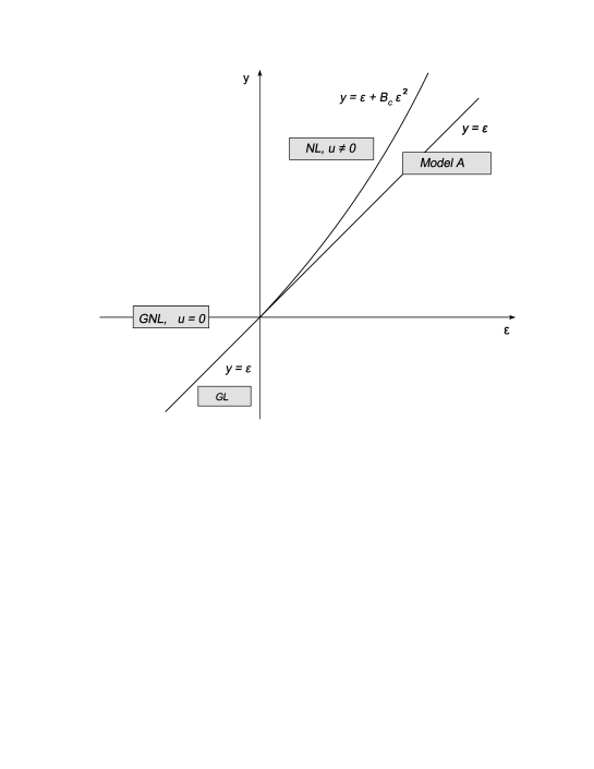
Figure 2: Regions of stability of the fixed points of the extended model (9), (10). The region labelled GNL (Gaussian nonlocal) corresponds to the fixed point with vanishing interaction ($d>4$) and purely nonlocal correlation function of the noise; the label NL, $u\neq 0$ refers to the nonlocal regime II of the extended model; the first-order boundary between the latter and the region of stability of the universality class of model A (the local regime I of the extended model) is $y=\varepsilon$ and the improved boundary is $y=\varepsilon+B_{c}\varepsilon^{2}$. The boundary between the universality class of model A and that of the linear model driven by the random noise with local correlations only – labelled GL (Gaussian local) – is the negative $y$ axis.

Furthermore, we can see that the fixed point with both $u_{*}\neq 0$ and $w_{*}\neq 0$ also exists for the beta functions (17x); we denote it as point II. Indeed, $\beta_{u_{*}}=0$ and $u_{*}\neq 0$ gives $u_{*}(1+w_{*})=\varepsilon/a$, substituting in $\beta_{w_{*}}=0$ and assuming $w_{*}\neq 0$ gives

$$0=-B\varepsilon^{2}+b(1+w_{*})[u_{*}(1+w_{*})]^{2}=\varepsilon^{2}\left\{-B+b(1+w_{*})/a^{2}\right\},$$

so that at the fixed point

$$w_{*}=-1+Ba^{2}/b,\qquad u_{*}=\varepsilon b/Ba^{3}$$ (17z)

with corrections of order $O(\varepsilon)$ and $O(\varepsilon^{2})$ respectively.

The $\Omega$ matrix at this point is:

$$\beta_{uu} = au_{*}(1+w_{*})=\varepsilon,$$

$$\beta_{uw} = au^{2}_{*}=\varepsilon^{2}b^{2}/B^{2}a^{5},$$

$$\beta_{wu} = 2u_{*}b\,w_{*}(1+w_{*})^{3}=2bw_{*}(\varepsilon/a)\,(a^{2}B/b)^{2},$$

$$\beta_{ww} = 3w_{*}bu^{2}_{*}(1+w_{*})^{2}=3bw_{*}(\varepsilon/a)^{2}.$$ (17aa)

Thus the $\Omega$ matrix has the form

$$\Omega=\varepsilon\,\left(\matrix{\alpha&{\cal A}\varepsilon\cr\beta&{\cal B}\varepsilon\cr}\right).$$ (17ab)

Although the elements in the right column are small in $\varepsilon$ in comparison to the left column, they are needed to find the eigenvalues to leading order. It is important that the $O(\varepsilon^{2})$ corrections to the left elements are not needed (they give only corrections), despite the fact that they would be of the same order as the right elements.

The eigenvalues are:

$$\Omega_{1}=\alpha\varepsilon+O(\varepsilon^{2}),\qquad\Omega_{2}=({\cal B}-\beta{\cal A}/\alpha)\varepsilon^{2}+O(\varepsilon^{3}).$$ (17ac)

The point is IR-attractive if $\Omega_{1,2}>0$. Substituting (17aa), (17z) gives: $\varepsilon>0$, $B>b/a^{2}$.

Thus the curve $y=\varepsilon+B_{c}\varepsilon^{2}$ with $B_{c}=b/a^{2}$ is the boundary between the regions of IR-stability for the point I ($\varepsilon>0$, $B<b/a^{2}$) and the new nonlocal point II ($\varepsilon>0$, $B>b/a^{2}$). There is neither gap nor overlap (at least in this approximation).

The physics requires that the coordinates of any physical fixed point, $u_{*}$ and $w_{*}$, be non-negative ($u$ and $uw$ are amplitudes in pair correlators). One can check that this condition is automatically satisfied in the region of their IR stability. For example, $w_{*}>0$ in (17z) gives $B>b/a^{2}$, which is also $\Omega_{2}>0$, and so on.

The resulting pattern of the regions of stability of the nontrivial fixed points of the model (9), (10), shown in figure 2, is as follows: the quadrant $\varepsilon>0$, $y>0$ is divided into two parts by the parabola $y=\varepsilon+B_{c}\varepsilon^{2}$ with $B_{c}=b/a^{2}$. The part below it is the region of IR stability of the point I (universality class of the equilibrium model A); it includes the whole sector $\varepsilon>0$, $\varepsilon>y$. The part above it is the region of IR stability of the point II. It corresponds to a new nonequilibrium universality class, where the nonlocal term in the random force is important. It is worth noting that $B_{c}$ appears rather small: $b=\ln(4/3)\approx 0.287683$ and $B_{c}=\ln(4/3)/9\approx 0.032$.

5 Scaling behaviour in the IR range

Existence of IR-attractive fixed points implies scaling behaviour with definite critical dimensions $\Delta_{F}$ of all quantities $F$ (fields and parameters):

$$\Delta_{F}=d^{k}_{F}+\Delta_{\omega}d^{\omega}_{F}+\gamma_{F}^{*},\qquad\Delta_{\omega}=2+\gamma_{\sigma}^{*},$$ (17ad)

where $d^{k,\omega}_{F}$ are the canonical dimensions of $F$, given in table 1, and $\gamma_{F}^{*}$ is the value of $\gamma_{F}$ at the fixed point in question; see e.g. [21, 26]. In the case at hand $\gamma_{F}^{*}=\gamma_{F}(u_{*},w_{*})$.

In particular, for the pair correlator of the field $\varphi$ this gives:

$$\langle\varphi({\bf x}+{\bf r},t+t^{\prime})\varphi({\bf x},t^{\prime})\rangle=r^{-2\Delta_{\varphi}}\,{\cal F}\left(\tau_{0}\,{r^{\Delta_{\tau}}},\,t/r^{\Delta_{\omega}}\right).$$ (17ae)

This is the leading term of the asymptotic behaviour in the IR range, determined by the inequalities $k\sim 1/r\ll\Lambda$, where $\Lambda$ is the UV momentum scale defined by the relation $u_{0}\sim\Lambda^{y}$. ${\cal F}$ is a universal scaling function of two arguments, which are supposed to be of order unity; this completes the definition of the IR range: $\tau_{0}\,{r^{\Delta_{\tau}}}\sim 1$, $t/r^{\Delta_{\omega}}\sim 1$. (In the free theory we would have $\tau_{0}r^{2}\sim 1$, $t/r^{2}\sim 1$). The correct canonical dimensions in (17ae) are guaranteed by the amplitudes built from IR irrelevant parameters $\sigma$ and $\Lambda$, not shown explicitly. One usually assumes that ${\cal F}$ has finite limits for $\tau_{0}=0$ (that is, exactly at the critical point) and/or $t=0$ (equal-time correlator). Then from (17ae) one obtains

$$\langle\varphi({\bf x}+{\bf r},t)\varphi({\bf x},t)\rangle=r^{-2\Delta_{\varphi}}.$$ (17af)

From the general expression (17ad), canonical dimensions $d^{k,\omega}_{F}$ from the table 1 and the relations (17s) we obtain

$$\Delta_{\varphi}=1-\varepsilon/2+(\gamma_{3}+\gamma_{2}-\gamma_{1})/2,\quad\Delta_{\omega}=2+\gamma_{2}-\gamma_{3},$$

$$\Delta_{\varphi^{\prime}}=3-\varepsilon/2+(\gamma_{1}+\gamma_{2}-\gamma_{3})/2,\quad\Delta_{\tau}=2-\gamma_{3}+\gamma_{5}.$$ (17ag)

Table 1: Canonical dimensions of the fields and parameters; $d=4-\varepsilon$.

$F$	$\varphi$	$\varphi^{\prime}$	$v_{i}$	$v_{i}^{\prime}$	$\sigma_{0},\sigma$	$\nu_{0},\nu$	$\!m,\mu,\Lambda\!$	$\tau$	$\lambda_{0}$	$w_{0}$	$g_{0}$	$\lambda,w,g$
$d_{F}^{k}$	${d\over 2}-1$	${d\over 2}-1$	$-1$	$\!d+1\!$	2	$-2$	1	2	$4-d$	$d-4+y$	$y^{\prime}$	0
$d_{F}^{\omega}$	0	1	1	$-1$	$-1$	1	0	0	0	0	0	0
$d_{F}$	${d\over 2}-1$	${d\over 2}+1$	1	$\!d-1\!$	0	0	1	2	$4-d$	$d-4+y$	$y^{\prime}$	0

In the leading approximation the anomalous dimensions have the forms

$$\gamma_{1}=b\,u^{2}(1+w)^{3},\quad\gamma_{2}=b\,u^{2}(1+w)^{2},\quad\gamma_{3}=u^{2}(1+w)^{2}/6,$$

$$\gamma_{4}=-3u(1+w),\quad\gamma_{5}=-u(1+w)$$ (17ah)

with $b=\ln(4/3)$. For $w=0$ these expressions coincide with the results known for the model A; see e.g. [21].

Consider first the fixed point I with $u_{*}=\varepsilon/a+O(\varepsilon^{2})$ and $w_{*}=0$. The local model ($w=0$) does not generate nonlocal counterterms and is “closed with respect to renormalization.” As a result, $w_{*}$ vanishes identically, the dimensions (17ag) are independent of $y$ and coincide with their analogs of the model A to all orders of the $\varepsilon$ expansion. For the model A, the fluctuation-dissipation theorem gives the exact relation $\gamma_{1}^{*}=\gamma_{2}^{*}$, so that these quantities disappear from the expression for $\Delta_{\varphi}$ in (17ag), while the dimensions $\gamma_{\varphi,\tau,u}^{*}$ (and hence $\Delta_{\varphi,\tau}$) coincide with their counterparts in the static $\lambda\varphi^{4}$ model; see e.g. [21, 22].

The standard notation for the equilibrium case is

$$\Delta_{\varphi}=d/2-1+\eta/2,\quad\Delta_{\tau}=1/\nu,\quad\Delta_{\omega}=z,$$ (17ai)

while for $\varphi^{\prime}$ the above identities give $\Delta_{\varphi^{\prime}}=\Delta_{\varphi}+z=d/2-1+z+\eta/2$. The static exponents $\eta$ and $\nu$ are well known from $4-\varepsilon$, $2+\varepsilon$ and $1/N$-expansions, real-space RG (all augmented by various summations), high-temperature expansions for the Ising model (considered most reliable), Monte-Carlo simulations. The values recommended by [21, 22] are $\eta=0.0375\pm 0.0025$ and $\nu=0.6310\pm 0.0015$ (Borel summation of 5-order results). For $z$ only two terms of the $4-\varepsilon$ expansion are known: $z=2+0.726(1-0.1885\varepsilon)\eta$ [34]; there are also leading-order results in $2+\varepsilon$ and $1/N$-expansions (see the references in [19, 20, 21]).

To avoid possible misunderstandings, it is worth noting that the scaling behaviour of the model A and the extended model (11) near its fixed point I coincide only to the leading orders given by the expressions (17ae), (17af). The corrections to those expressions are different. In particular, the leading correction from the UV range has the form $\left[1+c_{1}(k/\Lambda)^{\Omega_{1}}+c_{2}(k/\Lambda)^{\Omega_{2}}\right]$, where $\Omega_{1,2}$ are the eigenvalues of matrix $\Omega$ for the fixed point I given in (17y). One of them involves the parameter $y$ which is absent in the pure model A.

Let us turn to the nonlocal regime of the extended model (11), described by the fixed point II. Substituting (17ah) and (17z) into (17ag) gives

$$\Delta_{\varphi} = 1-\varepsilon/2+(\varepsilon^{2}/2)(1/54+b/9-B)+O(\varepsilon^{3}),$$

$$\Delta_{\varphi^{\prime}} = 3-\varepsilon/2+(\varepsilon^{2}/2)(-1/54+b/9-B)+O(\varepsilon^{3}),$$

$$\Delta_{\omega} = 2+(\varepsilon/3)^{2}(b-1/6)+O(\varepsilon^{3}),$$

$$\Delta_{\tau} = 2-\varepsilon/3+O(\varepsilon^{2}).$$ (17aj)

We recall that $B$ comes from the relation $y=\varepsilon+B\varepsilon^{2}$ and the nonlocal fixed point is IR-attractive when $B>b/9\approx 0.032$, see (17ac). Note that the dimension $\Delta_{\omega}=2+0.0013\varepsilon^{2}+O(\varepsilon^{3})$ appears surprisingly close to its canonical value $\Delta_{\omega}=2$.

Consider the real case $d=3$, then $y=1+B$ and the noise correlator is $1/r^{3-B}$. The exponent $\eta$, defined by the same “equilibrium” relation $\Delta_{\varphi}=d/2-1+\eta/2$, takes on the form $\eta=(1/54+b/9-B)\approx 0.05-B$. So $\eta$ can be made negative for reasonable $B$: in particular, for $B=1$ and noise correlator $1/r^{2}$ we have $\eta\approx-1$. In this respect, the nonequilibrium steady-state scaling differs from the equilibrium case, described by a local Landau–Ginzburg action: for the latter, the exact inequality $\eta>0$ can be derived from the unitarity of the corresponding pseudo-Euclidean quantum field theory [35]. Bearing in mind possible cosmological application of the model [30], it is tempting to note that $\eta=-1$ corresponds to the Zeldovich spectrum [36].

6 Inclusion of the velocity field

Let us turn to the full stochastic problem (2), (9), (10). The field theoretic action functional then becomes

$$S(\Phi)=S_{v}(v^{\prime},v)+\varphi^{\prime}D_{\varphi}\varphi^{\prime}/2+\varphi^{\prime}\left\{-\sigma_{0}\nabla_{t}\varphi+\partial^{2}\varphi-\tau_{0}\varphi-\lambda_{0}\varphi^{3}/6\right\},$$ (17ak)

where

$$S_{v}(v^{\prime},v)=v^{\prime}D_{v}v^{\prime}/2+v^{\prime}\left\{-\nabla_{t}+\nu_{0}\partial^{2}\right\}v$$ (17al)

is the action functional for the stochastic problem (2), $D_{\varphi}$ and $D_{v}$ are the correlation functions of the random forces $f$ and $f_{i}$, respectively, $\nabla_{t}=\partial_{t}+v_{i}\partial_{i}$, and all the required integrations over $x=\{t,{\bf x}\}$ and summations over the vector indices are understood. The new full set of fields $\Phi=\{\varphi,\varphi^{\prime},v_{i},v^{\prime}_{i}\}$ involves the auxiliary vector field $v_{i}^{\prime}$. It is also transverse, $\partial_{i}v_{i}^{\prime}=0$, which allows one to omit the pressure term on the right-hand side of relation (17al). Correlation function $D_{\varphi}$ is given by (10), while $D_{v}$ will be taken in the form

$$\langle f_{i}(x)f_{j}(x^{\prime})\rangle = g_{0}\nu_{0}^{3}\,\delta(t-t^{\prime})k^{4-d-y^{\prime}}P_{ij}({\bf k}),$$ (17am)

where $P_{ij}({\bf k})=\delta_{ij}-k_{i}k_{j}/k^{2}$ is the transverse projector, $y^{\prime}$ a new arbitrary parameter analogous to $y$ from (10), $g_{0}\sim\Lambda^{y^{\prime}}$ is a new positive coupling constant, and the factor $\nu_{0}^{3}$ is explicitly isolated for convenience. The IR cutoff at $k=m$ is also implied. Canonical dimensions of all the new parameters and their future renormalized counterparts are given in table 1.

The stochastic Navier–Stokes equation (2) with a power-law noise spectrum was introduced a long ago [23, 24, 25] and is by now very well studied, at least for small values of $y^{\prime}$. The two-loop results have been derived recently in [37]. Detailed exposition of the RG approach can be found in [21, 26]; below we confine ourselves to only the necessary information.

The model (17al) is logarithmic (the coupling constant $g_{0}$ is dimensionless) at $y^{\prime}=0$, and the UV divergences have the form of the poles in $y^{\prime}$ in the correlation functions of the fields $v$, $v^{\prime}$. Dimensional analysis, augmented by some additional considerations (Galilean symmetry and structure of the vertex), shows that for all $d>2$, the superficial UV divergences, whose removal requires counterterms, are present only in the 1-irreducible function $\langle v^{\prime}v\rangle$, and the corresponding counterterm reduces to the form $v^{\prime}\partial^{2}v$. Owing to the form of the vertex (the derivative can always be moved onto $v^{\prime}$ using integration by parts), the divergence in the function $\langle v^{\prime}v^{\prime}\rangle$ (allowed by dimension for $d<4$) is in fact absent for all $d>2$. So the local counterterm $v^{\prime}v^{\prime}$, analogous to $\varphi^{\prime}\varphi^{\prime}$ in (11), is not needed here. For this reason, we did not include the constant contribution to (17am), in contrast to its scalar counterpart (10). Then for the complete elimination of the UV divergences it is sufficient to perform the multiplicative renormalization of the parameters $\nu_{0}$ and $g_{0}$ with the only independent renormalization constant $Z_{\nu}$:

$$\nu_{0}=\nu Z_{\nu},\qquad g_{0}=g\mu^{y^{\prime}}Z_{g},\qquad Z_{g}=Z_{\nu}^{-3}.$$ (17an)

Here $\mu$ is the reference mass in the MS scheme, $g$ and $\nu$ are renormalized analogs of the bare parameters $g_{0}$ and $\nu_{0}$, and $Z=Z(g,y^{\prime},d)$ are the renormalization constants. In contrast to the model (11), no renormalization of the fields is needed, $Z_{v.v^{\prime}}=1$. The relation between the $Z$’s in (17an) results from the absence of renormalization of the noise term in (17al). Now the standard RG equations are readily derived, the corresponding function $\beta_{g}=\widetilde{\cal D}_{\mu}g$ in the one-loop approximation is

$$\beta_{g}(g)=g(-y^{\prime}+3\gamma_{\nu})=g\left\{-y^{\prime}+\frac{3(d-1)S_{d}\,g}{4(d+2)(2\pi)^{d}}\right\}+O(g^{3})$$ (17ao)

where $S_{d}=2\pi^{d/2}/\Gamma(d/2)$ is the area of the unit sphere in $d$ dimensions. From (17ao) we immediately conclude that for $y^{\prime}>0$, the model has an IR attractive nontrivial fixed point $g_{*}>0$ ($\beta_{g}(g_{*})=0$, $\beta_{g}^{\prime}(g_{*})>0$), while for $y^{\prime}<0$ the IR attractive fixed point is Gaussian, $g_{*}=0$ (that is, the nonlinearity in (2) is IR irrelevant). From the first equality in (17ao), which follows from the relation between the $Z$’s in (17an), the value of $\gamma_{\nu}$ at the nontrivial fixed point is found exactly: $\gamma_{\nu}^{*}=y^{\prime}/3$ (no corrections of order $(y^{\prime})^{2}$ and higher). As a result, critical dimensions of the frequency and the fields are also found exactly:

$$\Delta_{\omega}=2-y^{\prime}/3,\quad\Delta_{v}=1-y^{\prime}/3,\quad\Delta_{v^{\prime}}=d-1+y^{\prime}/3.$$ (17ap)

These results remain intact in the full model (17ak), because the inclusion of the scalar fields does not affect the velocity (the field $\varphi$ is “passive”). We thus conclude that for $y^{\prime}<0$, where the IR behaviour of the velocity becomes Gaussian, the scaling regimes of the full problem (17ak) are described by the fixed points I and II from section 4 depending on the relation between $y$ and $\varepsilon=4-d$.

For $y^{\prime}>0$ the contributions of the velocity field become IR relevant, and the RG analysis of the full problem (17ak), (17al) is needed. For $d>4$, where no local counterterm $\varphi^{\prime}\varphi^{\prime}$ is required, the model in question is formally equivalent to the stochastic model of the turbulent advection of a chemically active scalar field, studied earlier in [38]. We will be interested in the case $d<4$, where the local counterterm should be included from the very beginning to ensure multiplicative renormalizability. Then the UV divergences manifest themselves as poles in the full set of regulators $y$, $y^{\prime}$ and $\varepsilon=4-d$. Dimensional analysis and symmetry considerations show that, for all $d>2$, the full model is multiplicatively renormalizable, and the corresponding renormalized action has the form

$$S_{R}(\Phi) = S_{vR}(v^{\prime},v)+\varphi^{\prime}\left\{w\mu^{y-\varepsilon}k^{\varepsilon-y}+Z_{1}\right\}\varphi^{\prime}/2$$ (17aq)

$$+ \varphi^{\prime}\left\{-Z_{2}\sigma\nabla_{t}\varphi+Z_{3}\partial^{2}\varphi-\tau Z_{5}\varphi-Z_{4}\lambda\mu^{\varepsilon}\varphi^{3}/6\right\},$$

where $S_{vR}(v^{\prime},v)$ is the renormalized analog of the action (17al) expressed in renormalized variables using relation (17an). The renormalization constants $Z_{1}$–$Z_{5}$ now contain the poles in the full set of regulators $y$, $y^{\prime}$, $\varepsilon=4-d$ and, in comparison to (11), depend on two additional dimensionless couplings $g$ and $s=\sigma\nu$. One can easily see that the relations (12), (13) for the new constants $Z_{F}$ and (17r), (17s) for the corresponding anomalous dimensions $\gamma_{F}$ remain valid in the extended renormalized model (17aq). The RG equation takes on the form

$$\left\{{\cal D}_{RG}+N_{\varphi}\gamma_{\varphi}+N_{\varphi^{\prime}}\gamma_{\varphi^{\prime}}+N_{v}\gamma_{v}+N_{v^{\prime}}\gamma_{v^{\prime}}\right\}\,G^{R}(e,\mu,\dots)=0,$$ (17ar)

where ${\cal D}_{RG}$ is the operation $\widetilde{\cal D}_{\mu}$ expressed in the renormalized variables:

$${\cal D}_{RG}\equiv{\cal D}_{\mu}+\beta_{g}\partial_{g}+\beta_{u}\partial_{u}+\beta_{w}\partial_{w}+\beta_{s}\partial_{s}-\gamma_{\nu}{\cal D}_{\nu}-\gamma_{\tau}{\cal D}_{\tau},$$ (17as)

with $\beta_{g}$ from (17ao), $\beta_{u,w}$ from (16), and the new function $\beta_{s}$ is

$$\beta_{s}=-s\gamma_{s}=-s[\gamma_{\nu}+\gamma_{\sigma}]=-s[\gamma_{\nu}+\gamma_{2}-\gamma_{3}].$$ (17at)

Furthermore, it is easily checked that in the leading order, the anomalous dimensions $\gamma_{1,2,4,5}$ remain the same as in the model without velocity and can be taken from (17ah). On the contrary, $\gamma_{3}$ acquires an additional $O(g)$ term, in comparison to which the $O(u^{2})$ term in (17ah) is only a correction and should be neglected. So the leading-order expression for $\gamma_{3}$ becomes

$$\gamma_{3}=\frac{3gs^{2}}{64\pi^{2}(s+1)}+O(g^{2},u^{2}).$$ (17au)

As usual, scaling regimes of the full model are associated with the IR attractive fixed points, whose coordinates are found from the equations $\beta_{x}=0$ with $x=\{g,s,u,w\}$. Due to passivity of the field $\varphi$, the function $\beta_{g}$ is independent of $x=\{s,u,w\}$ and the corresponding elements $\partial\beta_{g}/\partial x$ of the matrix $\Omega$ vanish. Thus $\Omega$ is triangular, its elements $\partial\beta_{x}/\partial g$ with $x=\{s,u,w\}$ do not affect the eigenvalues, and we can set $g=g_{*}$ in the functions $\beta_{x}$ with $x\neq g$ from the very beginning. Now we are treating $\varepsilon=4-d$ as one of the small expansion parameters, and in the leading-order approximation we should set $d=4$ in (17ao) and $g_{*}$. In the leading approximation, the function $\beta_{s}$ is independent of $u$ and $w$, and the elements $\partial\beta_{s}/\partial x$ with $x=\{u,w\}$ also vanish. The element $\partial\beta_{s}/\partial s$ coincides with one of the eigenvalues of $\Omega$. It is easy to see that, for $y^{\prime}>0$, this eigenvalue $\partial\beta_{s}/\partial s$ cannot be positive for $s_{*}=0$, so that the condition $\beta_{s}=0$ implies $\gamma_{\nu}+\gamma_{2}-\gamma_{3}=0$, which in our approximation gives $3s_{*}^{2}-s_{*}-1=0$. Physical considerations require $s_{*}>0$, which finally gives $s_{*}=(1+\sqrt{13})/6\approx 0.7676$. Since the elements $\partial\beta_{x}/\partial s$ with $x=\{u,w\}$ are again irrelevant in the analysis of the remaining eigenvalues, we can set $s=s_{*}$ in $\beta_{u,w}$. We are left with the system of two equations, $\beta_{u,w}=0$, where

$$\beta_{u} = u[-\bar{\varepsilon}+au(1+w)+O(g^{2},u^{2})],$$

$$\beta_{w} = w[-\bar{y}+\bar{\varepsilon}+bu^{2}(1+w)^{3}+O(g^{3},u^{3})].$$ (17av)

Here we have denoted

$$\bar{\varepsilon}=\varepsilon-2y^{\prime}/3,\qquad\bar{y}=y-2y^{\prime}/3.$$ (17aw)

Up to the notation, this system coincides with that describing the model without velocity, equation (17w), and its fixed points and their regions of stability can immediately be inferred from the results of section 4. In order to have a regular expansion we again set $\bar{y}=\bar{\varepsilon}+\bar{B}\bar{\varepsilon}^{2}$, while $\bar{\varepsilon}$ and $y^{\prime}$ are of the same order. (From the relation $\bar{\varepsilon}-\bar{y}=\varepsilon-y$ one obtains $B\varepsilon^{2}=\bar{B}\bar{\varepsilon}^{2}$. We could also write $y^{\prime}=B^{\prime}\bar{\varepsilon}$, but this is not necessary.) Now we can identify two fixed points, which we denote III and IV, corresponding to completely new universality classes.

The point III corresponds to a purely local model: $w_{*}=0$ to all orders of the perturbative expansion, and $u_{*}=\bar{\varepsilon}/a$ with corrections $O(\bar{\varepsilon}^{2})$. It is IR attractive for $\bar{\varepsilon}>0$ and $\bar{B}<b/a^{2}$ (we recall that $a=3$ and $b=\ln(4/3)$). For the point IV, one obtains $w_{*}=-1+\bar{B}a^{2}/b$ and $u_{*}=\bar{\varepsilon}b/\bar{B}a^{3}$, with corrections of order $O(\bar{\varepsilon})$ and $O(\bar{\varepsilon}^{2})$ respectively. It is IR attractive for $\bar{\varepsilon}>0$, $\bar{B}>b/a^{2}$. The curve $\bar{y}=\bar{\varepsilon}+\bar{B}_{c}\bar{\varepsilon}^{2}$ with $\bar{B}_{c}=b/a^{2}\approx 0.032$ is the boundary between the regions of IR-stability for these two points.

For both these regimes, the relations $\beta_{v}=0$ and $v_{*}\neq 0$ imply

$$\gamma^{*}_{\sigma}=\gamma^{*}_{2}-\gamma^{*}_{3}=-\gamma^{*}_{\nu}=-y^{\prime}/3,$$ (17ax)

and the critical dimension of frequency is found exactly:

$$\Delta_{\omega}=2+\gamma^{*}_{\sigma}=2-\gamma^{*}_{\nu}=2-y^{\prime}/3,$$ (17ay)

in agreement with (17ap). Combining Eqs. (17s) and (17ax) gives

$$2\gamma^{*}_{\varphi}=\gamma^{*}_{3}+\gamma^{*}_{2}-\gamma^{*}_{1}=\gamma^{*}_{\nu}+2\gamma^{*}_{2}-\gamma^{*}_{1},$$

$$2\gamma^{*}_{\varphi^{\prime}}=\gamma^{*}_{3}+\gamma^{*}_{1}-\gamma^{*}_{2}=\gamma^{*}_{\nu}+\gamma^{*}_{1},$$ (17az)

which, along with (17ay), allows one to determine the dimensions $\Delta_{\varphi}=(d/2-1)+\gamma^{*}_{\varphi}$ and $\Delta_{\varphi^{\prime}}=(d/2-1)+\Delta_{\omega}+\gamma^{*}_{\varphi^{\prime}}$ in the second order of the $\varepsilon$ expansion without practical calculation of the two-loop corrections to $\gamma_{3}$ and $v_{*}$:

$$\Delta_{\varphi}=1-\varepsilon/2+y^{\prime}/6+b\bar{\varepsilon}^{2}/18,\quad\Delta_{\varphi^{\prime}}=3-\varepsilon/2-y^{\prime}/6+b\bar{\varepsilon}^{2}/18$$ (17ba)

for the fixed point III and

$$\Delta_{\varphi}=1-\varepsilon/2+y^{\prime}/6+b\bar{\varepsilon}^{2}/9-\bar{B}\bar{\varepsilon}^{2}/2,\quad\Delta_{\varphi^{\prime}}=3-\varepsilon/2-y^{\prime}/6+\bar{B}\bar{\varepsilon}^{2}/2$$ (17bb)

for the fixed point IV, with cubic-in-$\varepsilon$ corrections. (We recall that in counting the orders we imply $\varepsilon\sim\bar{\varepsilon}\sim y^{\prime}$, $\varepsilon-y\sim\varepsilon^{2}$). In fact, the expression for $\Delta_{\varphi^{\prime}}$ in (17bb) holds to all orders (no corrections of order $\varepsilon^{3}$ and higher), because $\gamma_{1}^{*}=y-\varepsilon=B\varepsilon^{2}$ exactly, as a consequence of the relations $\beta_{w}=0$ and $w_{*}\neq 0$. Finally, for the both points III and IV one obtains $\Delta_{\tau}=2+\varepsilon/3+y^{\prime}/9$, with quadratic corrections.

For $\bar{\varepsilon}<0$, the self-interaction of the scalar field becomes irrelevant ($u_{*}=0$), and we obtain two more fixed points, which correspond to the scalar field subject to a linear diffusion-advection equation, with the velocity ensemble given by the action $S_{v}(v^{\prime},v)$ from (17al). The regions $\bar{\varepsilon}>\bar{y}$ and $\bar{\varepsilon}<\bar{y}$ correspond to the local ($w_{*}=0$) and nonlocal correlator of the scalar noise, respectively. For the purely nonlocal case, the amplitude $w$ remains finite at the fixed point and can be eliminated from the action by appropriate rescaling of the fields $\varphi$ and $\varphi^{\prime}$.

The linear passive scalar case is very well understood within the RG framework (see e.g. chapter 2 in the book [26] and references therein). The only superficially divergent 1-irreducible correlation function is $\langle\varphi^{\prime}\varphi\rangle$ with the counterterm $\varphi^{\prime}\partial^{2}\varphi$, and the corresponding renormalization constant (in our notation identified with $Z_{\varphi}=Z_{\sigma}^{-1}$) is independent of the form of the noise correlator (the latter only determines the canonical dimensions). The absence of renormalization of the noise term results in the exact relation $Z_{\varphi^{\prime}}=1$ (it is implied that the amplitude is scaled out from the action). Along with the relations (17ax) and (17ay), which remain valid for the passive linear case, this gives exact results for the dimensions:

$$\Delta_{\varphi}=d/2-1+y^{\prime}/3,\quad\Delta_{\varphi^{\prime}}=d/2+1-y^{\prime}/3,\quad\Delta_{\tau}=2,$$ (17bc)

which in the standard “equilibrium” notation corresponds to $\eta=y^{\prime}/3$ and $\nu=1/2$, different from their counterparts for the standard model A.

7 Conclusion

We have studied stochastic model that describes dynamics of a nonconserved scalar field (order parameter) near its critical point, subject to random external stirring and mixing, in $d$ spatial dimensions. The stirring was modelled by an additive random Gaussian noise with the pair correlation function $\propto\delta(t-t^{\prime})k^{4-d-y}$. The mixing was modelled by the convection term with a divergence-free (due to the incompressibility condition) velocity field, governed by the stochastic Navier–Stokes equation with a random Gaussian force with pair correlation function $\propto\delta(t-t^{\prime})k^{4-d-y^{\prime}}$. Possible scaling regimes of the model are associated with nontrivial IR attractive fixed points of the corresponding RG equations. Their coordinates, regions of stability, and the corresponding critical dimensions can be calculated within a systematic expansion in $y$, $y^{\prime}$ and $\varepsilon=4-d$ (or only $y$ and $\varepsilon=4-d$ for the model without velocity) with the additional assumption that $y-\varepsilon=O(\varepsilon^{2})$. Depending on the relations between those parameters, the model reveals several types of scaling regimes. Some of them are well known: model A of equilibrium critical dynamics and linear passive scalar field advected by a random turbulent flow, but there are three new nonequilibrium universality classes, associated with new nontrivial fixed points. In this sense, the critical behaviour of the model appears richer and less universal than that of the equilibrium critical dynamics.

The critical exponents (dimensions) for the new universality classes are derived in the second order of the expansion in $y$, $y^{\prime}$ and $\varepsilon$ (two-loop approximation).

It remains to note that the large-scale mixing ($y=y^{\prime}=4$) in three dimensions ($\varepsilon=1$) belongs to the universality class of the linear passive scalar with the nonlocal noise correlator and therefore corresponds to the dimensions (17bc). Of course, the results of our perturbative RG analysis are absolutely reliable and internally consistent only for small values of the expansion parameters $\varepsilon$, $y$ and $y^{\prime}$, while the possibility of their naive extrapolation to finite (and not small) real values is far from obvious. On the other hand, the observation that the $\varphi^{4}$-interaction becomes irrelevant for the large-scale forcing is reminiscent of the results derived in [13, 14]. There, it was argued that a non-random shear flow strongly suppresses critical fluctuations, and the behaviour of the system becomes close to mean field in the strong shear limit; see also discussion in [15].

Our analysis can be directly generalized to the cases of a $N$-component order parameter, presence of anisotropy, compressibility etc. The generalizations are straightforward but rather cumbersome (for the stochastic Navier–Stokes equation, see e.g. chapter 3 in the book [26] and references therein). On the contrary, the case of a conserved order parameter appears rather different from both the conceptual and technical viewpoints (namely, it involves two different dispersion laws: $\omega\sim k^{2}$ for the velocity and $\omega\sim k^{4}$ for the scalar). These issues will be addressed elsewhere.

Appendix A Calculation of the renormalization constants

Consider as an example the calculation of the constant $Z_{1}$ and the anomalous dimension $\gamma_{1}$ for the model (10) without the velocity field in detail. The leading contribution here is given by a two-loop Feynman graph, so this example is representative: calculation of the other renormalization constants (including the velocity field) can be performed in a similar way (for two-loop contributions) or is much easier (for one-loop graphs).

The 1-irreducible function $\Gamma\equiv\langle\varphi^{\prime}\varphi^{\prime}\rangle$ in the renormalized critical ($\tau=0$) theory to order $O(\lambda^{2})$ has the form

$$\Gamma=2\sigma\,\left\{w(k/\mu)^{y-\varepsilon}+Z_{1}\right\}+\frac{\lambda^{2}\mu^{2\varepsilon}}{6}\times{\rm Diagram},$$ (17bd)

where the first term is the noise correlator written in renormalized variables, $Z_{1}$ should be taken to order $O(\lambda^{2})$, 1/6 is the symmetry coefficient, $\lambda^{2}\mu^{2\varepsilon}$ comes from the vertex factors, dashed external ends correspond to fields $\varphi^{\prime}$ and the three identical lines correspond to bare propagators

$$\langle\varphi\varphi\rangle_{0}=\frac{2\sigma\,\left\{w\,(k/\mu)^{y-\varepsilon}+1\right\}}{\omega^{2}\sigma^{2}+k^{4}}$$ (17be)

in frequency-momentum representation and

$$\langle\varphi\varphi\rangle_{0}=\left\{w\,(k/\mu)^{y-\varepsilon}+1\right\}\,\frac{1}{k^{2}}\,\exp{(-k^{2}|t-t^{\prime}|/\sigma)}$$ (17bf)

in time-momentum representation. The second bare propagator

$$\langle\varphi\varphi^{\prime}\rangle_{0}=(-{\rm i}\sigma\omega+k^{2})^{-1}\to\theta(t-t^{\prime})\exp{(-k^{2}(t-t^{\prime})/\sigma)}$$ (17bg)

existing in the diagrammatic technique for the model (11) does not appear in this diagram. Within our accuracy, all $Z$’s occurring in the diagram (for example, $Z_{4}^{2}$ coming from renormalized vertices) have been replaced with unities.

The constant $Z_{1}$ will be found from the condition that it cancels the poles in $\varepsilon$ and $y$ which are present in the diagram, so the full expression (17bd) is regular in $\varepsilon$ and $y$ and finite for $\varepsilon=0$, $y=0$. This requirement determines $Z_{1}$ up to a regular part. We will use the minimal subtraction (MS) scheme where $Z_{1}=1+$ only poles in $\varepsilon$, $y$ and their linear combinations. In the model with two regulators like $\varepsilon$, $y$ there are subtleties in defining the MS scheme in higher orders (for example, is $\varepsilon/y$ a pole or a finite thing). We will work only in the leading order and can neglect these subtleties.

It is sufficient to calculate the diagram with the external frequency and momentum equal to zero. In the theory above the critical temperature ($\tau>0$) the IR regularization is provided by the replacement $k^{2}\to k^{2}+\tau$ in the denominator of (17bf)). This becomes impossible for the case $\tau\leq 0$, which we are mostly interested in here. The adequate language is then provided by the Legendre transform (effective action) and use of the loop expansion or the $1/N$ expansion instead of the primitive perturbation theory. This is not convenient, however, for the practical calculation of the renormalization constants. Fortunately, in the MS scheme the counterterms are polynomial in IR regulators, and the results obtained for them in the region $\tau>0$ can be directly used for $\tau\leq 0$; see e.g. the discussion section 3.36 in [21]. Furthermore, the constants $Z$ are independent on the specific choice of the IR regularization. From the calculational viewpoints, it is more convenient to set $\tau=0$ in the action (and in the propagator (17bf)) and cut off the momentum integrals at $k=m$ (by dimension, $\tau\sim m^{2}$). Integrals over frequencies (or times) are elementary, and one obtains:

$${\rm Diagram}={2\sigma}\!\!\int\limits_{k>m}\!\!\!\!\frac{d{\bf k}}{(2\pi)^{d}}\,\int\limits_{q>m}\!\!\!\!\frac{d{\bf q}}{(2\pi)^{d}}\,\frac{D(k)D(q)D(|{\bf k}+{\bf q}|)}{k^{2}q^{2}({\bf k}+{\bf q})^{2}[k^{2}+q^{2}+({\bf k}+{\bf q})^{2}]},$$ (17bh)

where we have denoted

$$D(k)\equiv[w\,(k/\mu)^{y-\varepsilon}+1].$$ (17bi)

The integrand in (17bh) depends only on three independent variables: the moduli $k={\bf k}$, $q={\bf q}$ and the angle $\vartheta$ between the directions ${\bf k}$ and ${\bf q}$, so that ${\bf k}{\bf q}=kq\cos\vartheta$. Thus the expression (17bh) can be written as a linear combinations of the integrals of the form

$$\int\limits_{k>m}\!\!\!\!\frac{d{\bf k}}{(2\pi)^{d}}\,\int\limits_{q>m}\!\!\!\!\frac{d{\bf q}}{(2\pi)^{d}}\dots=$$

$$\frac{S_{d}^{2}}{(2\pi)^{2d}}\,\int\limits_{m}^{\infty}\!\!\frac{dk}{k^{1+\varepsilon}}\int\limits_{m}^{\infty}\!\!\frac{dq}{q^{1+\varepsilon}}\langle\langle\frac{k^{2}q^{2}k^{\alpha_{1}}q^{\alpha_{2}}|{\bf k}+{\bf q}|^{\alpha_{3}}}{({\bf k}+{\bf q})^{2}[k^{2}+q^{2}+({\bf k}+{\bf q})^{2}]}\rangle\rangle$$ (17bj)

where each $\alpha_{i}$ is either 1 or $\varepsilon-y$, the brackets mean the averaging over the angle $\vartheta$ normalized as $\langle\langle 1\rangle\rangle=1$ and $S_{d}=2\pi^{d/2}/\Gamma(d/2)$ is the area of the unit sphere in the $d$-dimensional space.

From dimensional considerations it is obvious that for the integrals $I(m)$ in (17bj) we have

$$I(m)=m^{-2\varepsilon+\alpha_{123}}I(m=1),\qquad\alpha_{123}=\sum_{i}\alpha_{i}.$$ (17bk)

Thus

$${\cal D}_{m}I(m)=(-2\varepsilon+\alpha_{123})I(m),\qquad{\cal D}_{m}\equiv m\partial_{m}$$ (17bl)

and

$$I(m)=-m^{-2\varepsilon+\alpha_{123}}\frac{1}{(2\varepsilon-\alpha_{123})}{\cal D}_{m}I(m)|_{m=1}.$$ (17bm)

Here the pole is isolated explicitly. The expression ${\cal D}_{m}I(m)|_{m=1}$ is finite at $\varepsilon=y=0$, and we can set $\varepsilon=y=0$ in it. Then all these integrals become equal (all $\alpha_{i}$ also become 0).

The factors $m^{-2\varepsilon+\alpha_{123}}$ will form dimensionless ratios like $(m/\mu)^{O(\varepsilon)}$ or $(m/\mu)^{O(y)}$ with the $\mu$-dependent factors in expressions (17bd) and (17bi). Since we are interested only in the pole parts we will replace such ratios by unities. Thus we have to calculate

$${\cal R}=-{\cal D}_{m}I(m)|_{m=1,\varepsilon=y=0}.$$ (17bn)

Since $m$ appears in $I(m)$ only in the lower limits of integration, the differentiation gives

$${\cal R}=\int\limits_{1}^{\infty}dq\,\langle\langle\,\frac{q}{(1+q^{2}+2q\cos\vartheta)(1+q^{2}+q\cos\vartheta)}\,\rangle\rangle.$$ (17bo)

Here we have rescaled the variable $q/m\to q$, so that new $q$ is dimensionless and $m$ has disappeared. The factor 2 (there are two equal contributions since the integrand was symmetrical in $q$ and $k$) cancels with 1/2 from $[k^{2}+q^{2}+({\bf k}+{\bf q})^{2}]\to 2(1+q^{2}+q\cos\vartheta)$.

For $\varepsilon=0$, the prefactor ${S_{d}^{2}}/{(2\pi)^{2d}}$ in (17bj) is replaced with $1/64\pi^{4}$, while the angular averaging acquires the form

$$\langle\langle\dots\rangle\rangle=\frac{2}{\pi}\,\int^{\pi}_{0}\,\sin^{2}\vartheta\,\dots\,.$$

Calculating the resulting double integral gives ${\cal R}=(3/2)\ln(4/3)$.

Now consider the total cofactor which contains the poles in $\varepsilon$ and $y$. It comes from the denominators in (17bo) and has the form:

$${\cal P}=\left\{\frac{1}{2\varepsilon}+\frac{3w^{2}}{2\varepsilon-2(\varepsilon-y)}+\frac{3w}{2\varepsilon-(\varepsilon-y)}+\frac{w^{3}}{2\varepsilon-3(\varepsilon-y)}\right\}.$$ (17bp)

Then constant $Z_{1}$ which cancels the poles in (17bd) will have the form

$$Z_{1}=1-\frac{\lambda^{2}}{6}\,{\cal R}{\cal P}$$ (17bq)

($2\sigma$, being an overall factor in the first term of (17bd) and in (17bh), does not enter the expression for $Z_{1}$). The anomalous dimension is

$$\gamma_{1}=\tilde{\cal D}_{\mu}\ln Z_{1}$$

in renormalized variables using the chain rule we obtain ($u=\lambda/16\pi^{2}$)

$$\gamma_{1}=[\beta_{u}\partial_{u}+\beta_{w}\partial_{w}]\ln Z_{1}$$

with $\beta$ functions from (17t). In our approximation,

$$\tilde{\cal D}_{\mu}=-\varepsilon{\cal D}_{u}+(-y+\varepsilon){\cal D}_{w}\quad{\rm and}\quad\ln Z_{1}=-\frac{\lambda^{2}}{6}\,{\cal R}{\cal P}.$$

This finally gives

$$\gamma_{1}=\frac{\lambda^{2}}{6}\,{\cal R}(1+w)^{3}=u^{2}(1+w)^{3}\,\ln(4/3),$$ (17br)

as already stated in (17ah). For $w=0$ one obtains $\gamma_{1}=u^{2}\ln(4/3)$, in agreement with the result known for the model A; see e.g. [21, 34].

In the same manner we can derive the other results given in (17ah). For $\gamma_{2,3}$ the integral is quadratic and it should be expanded in the external frequency and momentum to $\Omega$ and $p^{2}$; the coefficients will be logarithmic integrals of the type (17bh) and we can proceed as before for (17bj). For $\gamma_{4,5}$ this is much simpler because the diagrams are one-loop ones, they are logarithmic, there is only one momentum ${\bf k}$ and the trick involving the differentiation ${\cal D}_{m}$ is not needed.

References

References

- [1] Bray A J 1994 Adv. Phys. 43 357
- [2] Onuki A 1997 J. Phys: Condens. Matt. 9 6119
- [3] Aronowitz J A and Nelson D R 1984 Phys. Rev. A 29 2012
-
[4]
Onuki A 1984 Phys. Lett. 101A 286
Onuki A and Takesue S 1986 Phys. Lett. 114A 133 -
[5]
Zhang F C, Valls O T and Mazenko G F 1985
Phys. Rev. B 31 1579
Zhang F C, Valls O T and Mazenko G F 1985 Phys. Rev. B 31 4453
Zhang F C, Valls O T and Mazenko G F 1985 Phys. Rev. B 32 5807 -
[6]
Mazenko G F and Valls O T 1987 Phys. Rev. Lett.
59 680
Mazenko G F, Valls O T and Zanetti M 1988 Phys. Rev. B 38 520 -
[7]
Roland C and Grant M 1988 Phys. Rev. Lett.
60 2657
Roland C and Grant M 1989 Phys. Rev. B 39 11971 -
[8]
Bray A J 1989) Phys. Rev. Lett. 62 2841
Bray A J 1990 Phys. Rev. B 41 6724 - [9] Lacasta A M, Sancho J M and Sagués F 1995 Phys. Rev. Lett. 75 1791
-
[10]
Corberi F, Gonnella G and Lamura A 1999 Phys. Rev. Lett. 83, 4057
Corberi F, Gonnella G and Lamura A 2000 Phys. Rev. E 62 8064 -
[11]
Bray A J and Cavagna A 2000 J. Phys. A: Math. Gen.
33 L305
Cavagna A, Bray A J and Travasso R D M 2000 Phys. Rev. E 62 4702
Bray A J, Cavagna A and Travasso R D M 2000 Phys. Rev. E 64 012102
Bray A J, Cavagna A and Travasso R D M 2001 Phys. Rev. E 65 016104 - [12] Berthier L 2001 Phys. Rev. E 63 051503
-
[13]
Onuki A and Kawasaki K 1980 Progr. Theor. Phys.
63 122
Onuki A, Yamazaki K and Kawasaki K 1981 Ann. Phys. 131 217
Imaeda T, Onuki A and Kawasaki K 1984 Progr. Theor. Phys. 71 16 -
[14]
Beysens D, Gbadamassi M and Boyer L 1979
Phys. Rev. Lett 43 1253
Beysens D and Gbadamassi M 1979 J. Phys. Lett. 40 L565 -
[15]
Chan C K 1990 Chinese J. Phys. 28 75
Chan C K, Perrot F and D. Beysens 1988 Phys. Rev. Lett. 61 412
Perrot F, Chan C K and D. Beysens 1989 Europhys. Lett. 9 65 - [16] Berthier L, Barrat J-L and Kurchan J 2001 Phys. Rev. Lett. 86 2014
-
[17]
Satten G and Ronis D 1985 Phys. Rev. Lett 55
91
Phys. Rev. A 33 1986 - [18] Berti S, Boffetta G, Cencini M and Vulpiani A 2005 Phys. Rev. Lett. 95 224501
- [19] Halperin B I and Hohenberg P C 1977 Rev. Mod. Phys. 49 435
- [20] Folk R and Moser G Critical Dynamics: A Field Theoretical Approach 2006 J. Phys. A: Math. Gen., submitted
- [21] Vasil’ev A N 2004 The Field Theoretic Renormalization Group in Critical Behavior Theory and Stochastic Dynamics (Boca Raton: Chapman & Hall/CRC).
- [22] Zinn-Justin J 1989 Quantum Field Theory and Critical Phenomena (Oxford: Clarendon)
- [23] Forster D, Nelson D R and Stephen M J 1977 Phys. Rev. A 16 732
- [24] De Dominicis C and Martin P C 1979 Phys. Rev. A 19 419
-
[25]
Sulem P L, Fournier J D and Frisch U 1979
Lecture Notes in Physics vol 104 p 321
Fournier J D and Frisch U 1983 Phys. Rev. A 19 1000 -
[26]
Adzhemyan L Ts, Antonov N V and Vasiliev A N 1999
The Field Theoretic Renormalization Group in Fully Developed
Turbulence (London: Gordon & Breach)
Adzhemyan L Ts, Antonov N V and Vasiliev A N 1996 Usp. Fiz. Nauk 166 1257 [Phys. Usp. 39 1193] - [27] Kardar M, Parisi G and Zhang Y-C 1986 Phys. Rev. Lett. 56 889
- [28] Kraichnan R H 1959 Journ. Fluid Mech. 5 407
-
[29]
Schmittman B and Zia R K P 1995 Phase Transitions and
Critical Phenomena vol 17 ed C Domb and J Lebowitz (London: Academic)
p. 267
Zia R K P 2002 Acta Physica Slovaca 52 495
Täuber U C 2002 Acta Physica Slovaca 52 505
Täuber U C 2003 Adv. Solid State Phys. 43, 659
Janssen H-K and Täuber U C 2004 Ann. Phys. (NY) 315 147
Basu A and Frey E 2004 Phys. Rev. E 69 015101
Calabrese P and Gambassi A 2005 J. Phys. A: Math. Gen. 38 R133 -
[30]
Starobrinsky A A 1986 Current Topics in Field Theory,
Quantum Gravity and Strings (Lecture Notes in Physics vol 264) ed
H J de Vega and N Sanchez (Heidelberg: Springer) p 207
Winitzki S and Vilenkin A 2000 Phys. Rev. D 61 084008 -
[31]
Ma S-K 1976 Phys. Rev. Lett. 37 461
Swendsen R H 1982 Real-Space Renormalization ed T W Burkhardt and J M J van Leeuwen (New York: Springer) p 57 - [32] Adzhemyan L Ts, Honkonen J, Kompaniets M V and Vasil’ev A N 2005Phys. Rev. E 71 036305
-
[33]
Khmel’nitski D E 1975 Sov. Phys. JETP 41 981
Shalaev B N 1977 Sov. Phys. JETP 26 1204
Jayaprakash C and Katz H J 1977 Phys. Rev. B 16 3987
Janssen H-K, Oerding K and Sengespeick E 1995 J. Phys. A: Math. Gen. 28 6073 - [34] Antonov N V and Vasil’ev A N 1984 Theor. Math. Phys. 60 671
- [35] Polyakov A M 1968 ZhETF 55 1026
- [36] Zeldovich Ya B and Novikov I D 1974 The Structure and the Evolution of the Universe (Moscow: Nauka)
- [37] Adzhemyan L Ts, Antonov N V, Kompaniets M V and Vasil’ev A N 2003 Int. J. Mod. Phys. B 17 2137
-
[38]
Hnatich M 1990 Teor. Mat. Fiz. 83 374
Antonov N V, Nalimov M Yu, Hnatich M and Horvath D 1998 Int. Journ. Mod. Phys. B 12 1937