Zero modes of tight binding electrons on the honeycomb lattice

Abstract

Tight binding electrons on the honeycomb lattice are studied where nearest neighbor hoppings in the three directions are $t_{a},t_{b}$ and $t_{c}$, respectively. For the isotropic case, namely for $t_{a}=t_{b}=t_{c}$, two zero modes exist where the energy dispersions at the vanishing points are linear in momentum $k$. Positions of zero modes move in the momentum space as $t_{a},t_{b}$ and $t_{c}$ are varied. It is shown that zero modes exist if $\left|\left|\frac{t_{b}}{t_{a}}\right|-1\right|\leq\left|\frac{t_{c}}{t_{a}}\right|\leq\left|\left|\frac{t_{b}}{t_{a}}\right|+1\right|$. The density of states near a zero mode is proportional to $|E|$ but it is propotional to $\sqrt{|E|}$ at the boundary of this condition

The integer quantum Hall effect has been observed in grapheneNovoselov2005 ; Zhang2005 when the carriers are changed by the gate voltage. The quantization of the Hall effect is observed as $\sigma_{xy}=2n\frac{e^{2}}{h}$ with $n=\pm 1,\pm 3\cdots$, where the factor $2$ comes from the spin degrees of freedom. These quantum numbers are unusual, since in a usual case $n=0,\pm 1,\pm 2,\cdots$. This unusual quantum Hall effect was discussed in terms of relativistic Dirac theory Gusynin2005 . However it is more natural to be explained by the realization of the quantum Hall effect in periodic systemsTKNN1982 in the presence of zero modesHasegawa2006 ; Peres2006 . We will call zero modes instead of massless Dirac excitations in this paper because we do not consider relativistic particles. The energy spectrum and the density of states of the honeycomb lattice near half filling and in zero or small magnetic field are similar to these in the square lattice near half filling in a very strong magnetic field about half flux quantum per each unit cellHasegawa2006 .

At zero carrier concentration (i.e. half-filled electrons), the resistivity $\rho_{xx}$ is close to the quantum value $h/(4e^{2})=6.45k\Omega$ independent of temperatureNovoselov2005 , which has been also attributed to the zero modesNovoselov2005 ; Zhang2005 ; Ziegler1998 .

The existence of zero modes has also been proposed for the quasi-two-dimensional organic conductor $\alpha$-(BEDT-TTF)₂I₃. The conductivity under pressure is almost constant in a wide range of temperatureTajima2002 . Pertinent numerical computations performed by Kobayashi et al.Kobayashi2004 found that, for certain range of parameters, the Fermi surfaces become points and the density of states is proportional to energy at 3/4 filling of electrons. The existence of zero modes was also confirmed by the band structure calculationIshibashi2006 ; Kino2006 . The unit cell for the model of $\alpha$-(BEDT-TTF)₂I₃ has four non-equivalent sites. Katayama et al.Katayama2006 studied simpler model with two sites in the unit cell and they obtained a condition for zero modes.

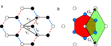
Figure 1: (color online) a. honeycomb lattice. Unit vectors are $\mathbf{v}_{1}=(\frac{3a}{2},-\frac{\sqrt{3}a}{2})$ and $\mathbf{v}_{2}=(\frac{3a}{2},\frac{\sqrt{3}a}{2}$). Three nearest neighbor hoppings are $t_{a}$, $t_{b}$ and $t_{c}$ b. The red hexagon is a Brillouin zone for the honeycomb lattice. The reciprocal lattice vectors are $\mathbf{G}_{1}=(\frac{2\pi}{3a},-\frac{2\pi\sqrt{3}}{3a})$ and $\mathbf{G}_{2}=(\frac{2\pi}{3a},\frac{2\pi\sqrt{3}}{3a})$. White circles are $\Gamma$ points. Brillouin zone can also be taken by the green diamond.

In this Letter we study a tight binding model on the honeycomb lattice and obtain the condition of $t_{a},t_{b}$ and $t_{c}$ for the existence of zero modes.

Unit cell of the honeycomb lattice contains two sublattices as shown in Fig. 1a. The Bravais lattice is a triangular lattice with

$$\mathbf{v}_{1} =(\frac{3a}{2},-\frac{\sqrt{3}a}{2}),$$ (1)

$$\mathbf{v}_{2} =(\frac{3a}{2},\frac{\sqrt{3}a}{2}),$$ (2)

where $a$ is a distance between nearest sites. We consider only nearest neighbor hoppings. There are three nearest neighbors for each site, $t_{a}$, $t_{b}$ and $t_{c}$ as shown in Fig.1. We study the generalized honeycomb lattice model where $t_{a}$, $t_{b}$ and $t_{c}$ are not necessarily equal. Under uniaxial pressure, $t_{a}$, $t_{b}$ and $t_{c}$ have different values for each other. For example, $t_{a}>t_{b}=t_{c}$ is expected, if the uniaxial pressure along the $x$ direction is applied. The Hamiltonian for the generalized honeycomb lattice is given by

$$\mathcal{H}=\sum_{\mathbf{r_{m}}}\Big{[} -t_{a}(a^{\dagger}_{\mathbf{r}_{m}}b_{\mathbf{r}_{m}}+h.c.)$$

$$-t_{b}(a^{\dagger}_{\mathbf{r}_{m}+\mathbf{v}_{1}}b_{\mathbf{r}_{m}}+h.c.)$$

$$-t_{c}(a^{\dagger}_{\mathbf{r}_{m}+\mathbf{v}_{2}}b_{\mathbf{r}_{m}}+h.c.)\Big{]}.$$ (3)

Using the Fourier transform

$$a_{\mathbf{r}_{m}} =\sum_{\mathbf{k}}e^{-i\mathbf{k}\cdot\mathbf{r}_{m}}a_{\mathbf{k}},$$ (4)

$$b_{\mathbf{r}_{m}} =\sum_{\mathbf{k}}e^{-i\mathbf{k}\cdot(\mathbf{r}_{m}+\mathbf{x})}b_{\mathbf{k}},$$ (5)

where $\mathbf{x}=(a,0)$, we obtain

$$\mathcal{H} =\sum_{\mathbf{k}}\Bigg{[}\Bigg{(}-t_{a}\exp({-ik_{x}})-t_{b}\exp\left(i\left(\frac{1}{2}k_{x}-\frac{\sqrt{3}}{2}k_{y}\right)\right)$$

$$-t_{c}\exp\left(i\left(\frac{1}{2}k_{x}+\frac{\sqrt{3}}{2}k_{y}\right)\right)\Bigg{)}a^{\dagger}_{\mathbf{k}}b_{\mathbf{k}}+h.c.\Bigg{]}.$$ (6)

The energy is given by

$$\epsilon_{\mathbf{k}}^{2} =t_{a}^{2}+t_{b}^{2}+t_{c}^{2}$$

$$+2t_{a}t_{b}\cos\left(\frac{3}{2}k_{x}-\frac{\sqrt{3}}{2}k_{y}\right)+2t_{a}t_{c}\cos\left(\frac{3}{2}k_{x}+\frac{\sqrt{3}}{2}k_{y}\right)$$

$$+2t_{b}t_{c}\cos\left(\sqrt{3}k_{y}\right).$$ (7)

If we perform a translation in the momentum space

$$(k_{x},k_{y})\rightarrow(k_{x}+\frac{2}{3}\pi,k_{y}),$$ (8)

and a replacement $t_{a}\rightarrow-t_{a}$ simultaneously, we get the same $\epsilon_{\mathbf{k}}$. Therefore we can take $t_{a}\geq 0$ without loss of generality. In a similar way one can take $t_{b}\geq 0$ and $t_{c}\geq 0$ without loss of generality by taking a translation in the momentum space,

$$(k_{x},k_{y})\rightarrow(k_{x}+\frac{1}{3}\pi,k_{y}\pm\frac{\sqrt{3}}{3}\pi).$$ (9)

The reciprocal lattice vectors are

$$\mathbf{G}_{1} =(\frac{2\pi}{3a},-\frac{2\pi\sqrt{3}}{3a}),$$ (10)

$$\mathbf{G}_{2} =(\frac{2\pi}{3a},\frac{2\pi\sqrt{3}}{3a}),$$ (11)

as shown in Fig. 1b. Let us write

$$\mathbf{k}=k_{1}\mathbf{G}_{1}+k_{2}\mathbf{G}_{2},$$ (12)

where

$$k_{1} =\frac{3}{4\pi}k_{x}-\frac{3}{4\sqrt{3}\pi}k_{y},$$ (13)

$$k_{2} =\frac{3}{4\pi}k_{x}+\frac{3}{4\sqrt{3}\pi}k_{y}.$$ (14)

The energy is

$$\epsilon_{\mathbf{k}}^{2} =t_{a}^{2}+t_{b}^{2}+t_{c}^{2}+2t_{a}t_{b}\cos(2\pi k_{1})$$

$$+2t_{a}t_{c}\cos(2\pi k_{2})+2t_{b}t_{c}\cos(2\pi(-k_{1}+k_{2})).$$ (15)

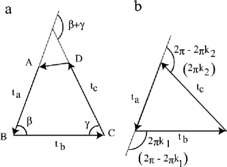
Figure 2: Graphical explanation for appearance of zero modes. (a) If $t_{a}$, $t_{b}$ and $t_{c}$ do not form a triangle, there are no zero modes and gaps at $E=0$ are open. (b) Zero modes exist when $t_{a}$, $t_{b}$ and $t_{c}$ form a triangle. Angles $k_{1}$ and $k_{2}$ are shown.

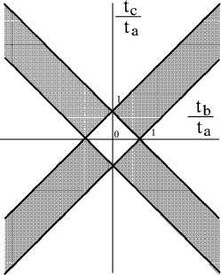
Figure 3: Zero modes exist in the filled region.

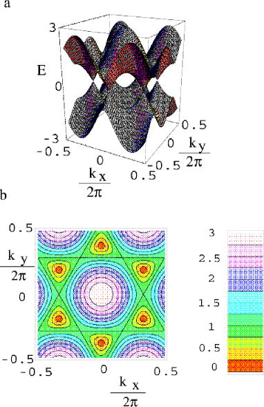
Figure 4: (color online) Energy dispersion for the isotropic case ($t_{a}=t_{b}=t_{c}=1$). (a) 3D plot and (b) contour plot.

Figure 5: Density of states of the electrons on a generalized honeycomb lattice.

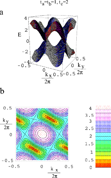
Figure 6: (color online) 3D plot (a) and the contour plot (b) of the energy of the generalized honeycomb lattice with $t_{a}=t_{b}=1$, $t_{c}=2$.

The minimum of $|\epsilon_{\mathbf{k}}|$ is obtained as follows. Consider the quadrangle ABCD in Fig. 2a. Then we have

$$|\overrightarrow{DA}|^{2} =|\overrightarrow{AB}+\overrightarrow{BC}+\overrightarrow{CD}|^{2}$$

$$=t_{a}^{2}+t_{b}^{2}+t_{c}^{2}$$

$$-2t_{a}t_{b}\cos\beta-2t_{b}t_{c}\cos\gamma-2t_{a}t_{c}\cos(\pi-\beta-\gamma)\geq 0.$$ (16)

Put

$$\beta =\pi-2\pi k_{1}$$ (17)

$$\gamma =\pi+2\pi(k_{1}-k_{2}),$$ (18)

then

$$t_{a}^{2}+t_{b}^{2}+t_{c}^{2}+2t_{a}t_{b}\cos(2\pi k_{1})$$

$$+ 2t_{a}t_{c}\cos(2\pi k_{2})+2t_{b}t_{c}\cos(2\pi(k_{1}-k_{2}))\geq 0$$ (19)

The equality is satisfied when $t_{a}$, $t_{b}$ and $t_{c}$ form a triangle which can be seen in Fig. 2b., i.e.,

$$\cos(2\pi k_{1}) =\frac{t_{c}^{2}-t_{a}^{2}-t_{b}^{2}}{2t_{a}t_{b}}$$ (20)

$$\cos(2\pi k_{2}) =\frac{t_{b}^{2}-t_{a}^{2}-t_{c}^{2}}{2t_{a}t_{c}}$$ (21)

$$\cos(2\pi(k_{1}-k_{2})) =\frac{t_{a}^{2}-t_{b}^{2}-t_{c}^{2}}{2t_{b}t_{c}}$$ (22)

The triangle can be formed when

$$\left|\frac{|t_{b}|}{|t_{a}|}-1\right|\leq\frac{|t_{c}|}{|t_{a}|}\leq\left|\frac{|t_{b}|}{|t_{a}|}+1\right|,$$ (23)

is satisfied. See Fig. 3.

In the isotropic case where $t_{a}=t_{b}=t_{c}$, zero modes are at $(k_{1},k_{2})=\pm(\frac{1}{3},\frac{2}{3})$, $(k_{1},k_{2})=\pm(\frac{2}{3},\frac{1}{3})$, and $(k_{1},k_{2})=\pm(-\frac{1}{3},\frac{1}{3})$ i.e. the corners of the first Brillouin zone, $(k_{x},k_{y})=\pm(\frac{2\pi}{3},\frac{2\sqrt{3}\pi}{9})$, $(k_{x},k_{y})=\pm(\frac{2\pi}{3},-\frac{2\sqrt{3}\pi}{9})$ and $(k_{x},k_{y})=\pm(0,\frac{4\sqrt{3}\pi}{9})$. See Fig. 4. The density of states is plotted in Fig. 5a.

If the parameters are in the boundary as seen in Fig. 3, two zero modes merge into a confluent point. For example, $\epsilon_{k}=0$ at confluent point $(k_{1}^{*},k_{2}^{*})=(0,1/2)$ for $t_{a}=t_{b}=1$, $t_{c}=2$ (Fig. 6). Near this point $\epsilon_{\mathbf{k}}$ is written as

$$\epsilon_{\mathbf{k}}\propto\pm\sqrt{c_{1}(k_{1}-k_{1}^{*})^{4}+c_{2}(k_{2}-k_{2}^{*})^{2}}$$ (24)

where $c_{1}$ and $c_{2}$ are constants. In this case the density of states near $E=0$ becomes

$$N(E)\propto\sqrt{|E|}.$$ (25)

See Fig. 5 b), while $N(E)\propto|E|$ in the case of two zero modes (Fig. 5a). When the inequality Eq.(23) is not satisfied, a finite gap opens at $E=0$ as shown in Fig. 5c.

In conclusion, we have studied the energy of tight binding electrons in the generalized honeycomb lattice and found the condition for the existence of zero modes. The zero modes exist at the corners of the hexagonal first Brillouin zone for the usual honeycomb lattice. Two zero modes moved to become a confluent point at the critical values of parameters $t_{a}$, $t_{b}$ and $t_{c}$, where $t_{a}$, $t_{b}$ and $t_{c}$ stop to form a triangle.

This work is supported by a Grant-in-Aid for the Promotion of Science and Scientific Research on Priority Areas (Grant No. 16038223) from the Ministry of Education, Culture, Sports, Science and Technology.

References

(1)
K.S. Novoselov, et al. Nature 438, 197 (2005).
(2)
Y. Zhang et al, Nature 438, 201 (2005).
(3)
V. P. Gusynin and S. G. Sharapov,
Phys. Rev. Lett. 95, 146801 (2005).
(4)
D. J. Thouless, M. Kohmoto, M. P. Nightingale, and M. den Nijs,
Phys. Rev. Lett. 49, 405 (1982);
M. Kohmoto, Ann. Phys. (NY) 160, 343 (1985).
(5)
Y. Hasegawa and M. Kohmoto,
cond-mat/0603345.
(6)
N. M. R. Peres, F. Guinea, and A. H. Castro Neto,
Phys. Rev. B 73, 125411 (2006).
(7)
K. Ziegler,
Phys. Rev. Lett. 80, 3113 (1998).
(8)
N. Tajima, A. Ebina-Tajima, M. Tamura, Y. Nishio and K. Kajita:
J. Phys. Soc. Jpn. 71 (2002) 1832.
(9)
A. Kobayashi, S. Katayama, K. Noguchi and Y. Suzumura,
J. Phys. Soc. Jpn. 73, 3135 (2004);
A. Kobayashi, S. Katayama and Y. Suzumura: J. Phys. Soc. Jpn. 74 (2005) 2897;
(10)
S. Ishibashi, T. Tamura, M. Kohyama and K. Terakura,
J. Phys. Soc. Jpn. 75, 015005 (2006).
(11)
H. Kino and T. Miyazaki,
J. Phys. Soc. Jpn. 75, 034704 (2006).
(12)
S. Katayama, A. Kobayashi and Y. Suzumura,
cond-mat/0601068.