Single Molecule Michaelis-Menten Equation beyond Quasi-Static Disorder

Abstract

The classic Michaelis-Menten equation describes the catalytic activities for ensembles of enzyme molecules very well. But recent single-molecule experiment showed that the waiting time distribution and other properties of single enzyme molecule are not consistent with the prediction based on the viewpoint of ensemble. It has been contributed to the slow inner conformational changes of single enzyme in the catalytic processes. In this work we study the general dynamics of single enzyme in the presence of dynamic disorder. We find that at two limiting cases, the slow reaction and nondiffusion limits, Michaelis-Menten equation exactly holds although the waiting time distribution has a multiexponential decay behaviors in the nondiffusion limit. Particularly, the classic Michaelis-Menten equation still is an excellent approximation other than the two limits.

The Michaelis-Menten (MM) mechanism Michaelis is widely used to understand the catalytic activities of various enzymes. According to this mechanism, a substrate S binds reversibly with an enzyme E to form a complex ES. ES then undergoes unimolecular decomposition to form a product P, and E is regenerated for the next cycle.

$$\textrm{E+S}\ \ \raisebox{-8.61108pt}{$\stackrel{{\scriptstyle\stackrel{{\scriptstyle\textrm{\small$k_{1}$}}}{{\textrm{\Large$\rightleftharpoons$}}}}}{{\textrm{\small$k_{-1}$}}}$}\ \ \textrm{ES}\xrightarrow{{k_{2}}}{\rm E}^{0}+{\rm P},\ \ \ {\rm E}^{0}\xrightarrow{{k}}{\rm E}$$ (1)

The rate of product formation $v$ on substrate concentration $[S]$ can be characterized by the MM equation Michaelis

$$v=\frac{v_{\rm max}[S]}{[S]+K_{\rm M}}$$ (2)

where $v_{\rm max}=k_{2}[E]_{\rm T}$ is the maximum generation velocity, $[E]_{T}=[E]+[ES]$ is the total enzyme concentration, and $K_{\rm M}=(k_{-1}+k_{P})/k_{1}$ is the Michaelis constant. Although the MM mechanism and equation have been found for almost a hundred years, they are still widely accepted and remain pillars of enzymology.

Even if the classic MM equation achieves considerable success, there are still many intriguing problems about the equation waiting to be answered. Particularly, the recent single-molecule fluorescence studies Lu ; Zhuang ; Oijen ; Yang ; Flomenbom found that catalytic rates of many enzymes are fluctuating with time due to conformational fluctuations. A natural question hence is why MM equation works well despite the broad distributions and dynamic fluctuations of single-molecule enzymatic rates. Recently Xie et al. tried to address this issue from view of points of single-molecule experiment English and theory Kou . In addition that the reciprocal of the first moment of $f(t)$, $\langle t\rangle^{-1}=v/[E]_{\rm T}$ follows MM equation well at any substrate concentration, the most remarkable discovery of their experiment is that the waiting time distributions $f(t)$ exhibit highly stretched multiexponential decays at high substrate concentration and monoexponential decays at low substrate concentration English . Xie et al. Kou attributed the nonexponential decay of $f(t)$ to dynamic disorder of the rate constants of the reactions in Eq. (1) caused by transitions among different enzyme conformations. They theoretically proved that the classic MM equation still holds at the single molecular level when the transition rates among the $ES$ conformations are slower than the catalytic rate $k_{2}$ (the quasi-static condition), even if $f(t)$ is no longer monoexponential decays at high substrate concentrations. Therefore one of following issues is whether we can still derive the MM equation beyond the quasi-static disorder. Xie et al. Kou indeed attempted to give an answer about it. But their effort ended in the two-state model for the algebraically complex in the multistate model. In this work, we propose that the classic MM equation holds under broader disorder conditions. Different from the discrete state model of Xie et al., a continuum diffusion-reaction model is used AgmonHopfield .

The conformational probability density for each enzyme state, $P_{\rm I}(x,t)$, in Eq. (1) can be obtained by three coupled diffusion-reaction equations with the potential [$V_{\rm I}(x)$] and the reaction terms [$k_{i}(x)$]

$$\frac{\partial}{\partial t}P_{\rm E}(x,t)=\left[{\cal L}_{\rm E}-k_{1\rm S}(x)\right]P_{\rm E}+k_{-1}(x)P_{\rm ES}$$

$$\frac{\partial}{\partial t}P_{\rm ES}(x,t)=\left[{\cal L}_{\rm ES}-k_{3}(x)\right]P_{\rm ES}+k_{1\rm S}(x)P_{\rm E}$$ (3)

$$\frac{\partial}{\partial t}P_{\rm E^{0}}(x,t)={\cal L}_{\rm E^{0}}P_{\rm E^{0}}+k_{2}(x)P_{\rm ES}$$

where

$${\cal L}_{\rm I}=D_{\rm I}\frac{\partial}{\partial x}\exp[-\beta V_{\rm I}(x)]\frac{\partial}{\partial x}\exp[\beta V_{\rm I}(x)],$$ (4)

and I$=$E, ES or E⁰, and $k_{3}(x)=k_{-1}(x)+k_{2}(x)$ and $k_{1S}(x)=k_{1}(x)[S]$ are defined for convenience. The diffusion coefficient $D_{\rm I}$ determines the rate of the conformational transition on the state $i$. The initial conditions are $P_{\rm ES}(x,0)=0$, $P_{\rm E^{0}}(x,0)=0$, and $P_{\rm E}(x,0)$ is the thermal equilibrium distribution with the potential $V_{\rm E}(x)$. In single molecule turnover experiment, the observation is the probability density of the waiting time for an enzymatic reaction $f(t)$, which is defined

$$f(t)=\int k_{2}(x)P_{\rm ES}(x)dx.$$ (5)

We first study the solutions of Eq. (Single Molecule Michaelis-Menten Equation beyond Quasi-Static Disorder) in two limiting cases: the slow reaction and the nondiffusion limits. In addition that the coupled diffusion-reaction equations have exact analytical solutions under these limits, this study would be useful in understanding the general solutions of Eq. (Single Molecule Michaelis-Menten Equation beyond Quasi-Static Disorder). Particularly, we will show that quasi-static condition proposed by Xie et al. is just one of case of the latter limit.
The slow reaction limit In this limit the processes of reactions is very slowly compared to processes of the enzyme conformational diffusion. Therefore the thermal distributions are always maintained during the courses of reactions. The solution to the diffusion-reaction equations then can be written as

$$P_{\rm I}(x,t)=P^{\rm eq}_{\rm I}(x)\rho_{\rm I}(t).$$ (6)

where $P^{\rm eq}_{\rm I}(x)\propto\exp[-\beta V_{\rm I}(x)]$, and $\beta^{-1}=k_{\rm B}T$, $k_{\rm B}$ is the Boltzmann’s constant, and $T$ is absolute temperature. Substituting them into Eq. (23) and considering that

$${\cal L}_{\rm I}P^{\rm eq}_{\rm I}(x)=0,$$ (7)

after simple calculations we get

$$f(t) = \rho_{\rm ES}(t)\int k_{2}(x)P^{\rm eq}_{\rm ES}(x)dx$$

$$= \frac{k^{1S}_{{\rm E}_{\rm eq}}k^{2}_{{\rm ES}_{\rm eq}}}{2A_{e}}\left[e^{(B_{\rm eq}+A_{\rm eq})t}-e^{(B_{\rm eq}-A_{\rm eq})t}\right],$$

where $A_{\rm eq}=\left[(k^{3}_{{\rm ES}_{\rm eq}}+k^{1S}_{{\rm E}_{\rm eq}})^{2}/4-k^{1S}_{{\rm E}_{\rm eq}}k^{2}_{{\rm ES}_{\rm eq}}\right]^{1/2}$ and $B_{\rm eq}=-(k^{3}_{{\rm ES}_{\rm eq}}+k^{1S}_{{\rm E}_{\rm eq}})/2$. Hence the reciprocal of the mean waiting time is

$$\frac{1}{\langle t\rangle}=\frac{k^{2}_{{\rm ES}_{\rm eq}}[S]}{[S]+M_{\rm eq}},$$ (9)

where $M_{\rm eq}=(k^{-1}_{{\rm ES}_{\rm eq}}+k^{2}_{{\rm ES}_{\rm eq}})/k^{1}_{{\rm E}_{\rm eq}}$. We can see that in this rapid diffusion limit, Eq. (9) is almost the same as the single molecule MM equation in the absence of dynamic disorder Kou except that the rate constants now are the mean values on their inner conformational coordinate.
The nondiffusion limit ($k_{i}^{-1}\ll\beta D_{\rm I}$) In this limit the reactions in Eq. (1) proceed so rapidly at the initial values of the slow coordinate $x$ that the distribution of $x$ is not restored by diffusion in the course of reactions. Then the diffusion terms in the diffusion reaction equations are neglected or $D_{\rm I}\approx 0$. The following calculations are simple and we immediately have

$$f(t)=\int P^{\rm eq}_{E}(x)\frac{k_{1S}(x)k_{2}(x)}{2A(x)}\left\{e^{[B(x)+A(x)]t}-e^{[B(x)-A(x)]t}\right\}dx$$ (10)

and

$$\frac{1}{\langle t\rangle}=\frac{\kappa_{\rm nd}[S]}{[S]+M_{\rm nd}}$$ (11)

where

$$\kappa_{\rm nd}^{-1}=\int dxP^{\rm eq}_{\rm E}(x)/k_{2}(x)dx,$$

$$M_{\rm nd}=\kappa_{\rm nd}\int P^{\rm eq}_{\rm E}(x)k_{3}(x)/\left[k_{1}(x)k_{2}(x)\right]dx,$$

where $A(x)=\left[(k_{1S}(x)+k_{3}(x))^{2}/4-k_{1S}(x)k_{2}(x)\right]^{1/2}$ and $B(x)=-(k_{3}+k_{1S})/2$.

We note that the expressions of the waiting distribution and the mean waiting time in the latter limit is very similar with the main conclusion [Eq. (31)] obtained by Xie et al. Kou . It is not unexpected because the quasi-static condition used by Xie et al. is included in our nondiffusion limit. But two new points are revealed in the present work. One is that, in addition to $k_{2}$, the other rates may also be allowed to fluctuating in time. The other and more interesting finding is that the unknown steady-state weight function $w(k_{2})$ introduced in prior by Xie et al. has a direct physical interpretation. To better understand the similarity between our calculation with them, we rewrite Eq. (10) by viewing $k_{2}$ as variable instead of $x$, and make use of the experimental observations English that both $k_{1}(x)$ and $k_{-1}(x)$ are independent of the conformational coordinate (the “wide reaction window” limit termed by Sumi and Marcus Sumi ), then we obtain the same expression as that Xie et al. solved by very complicated algebra operations.

$$f(t)=\int_{0}^{\infty}w(k_{2})\frac{k_{1}k_{2}[S]}{2A}\left[e^{(B+A)t}-e^{(B-A)t}\right]dk_{2},$$ (12)

while the weight function $w(k_{2})$ is related to the initial equilibrium distribution as follows,

$$w(k_{2})=P^{\rm eq}_{\rm E}\left[x^{-1}(k_{2})\right]\frac{dx}{dk_{2}},$$ (13)

where $x^{-1}(k_{2})$ is the inverse function of $k_{2}(x)$. In order to demonstrate the usage of this “microscopic” interpretation, we fit our theory by assuming that the potential $V_{\rm E}$ has a harmonic form with spring constant $k$, i.e.,

$$P_{\rm E}(x)=\frac{1}{\sqrt{2\pi}\sigma}\exp(-\frac{x^{2}}{2\sigma^{2}})$$ (14)

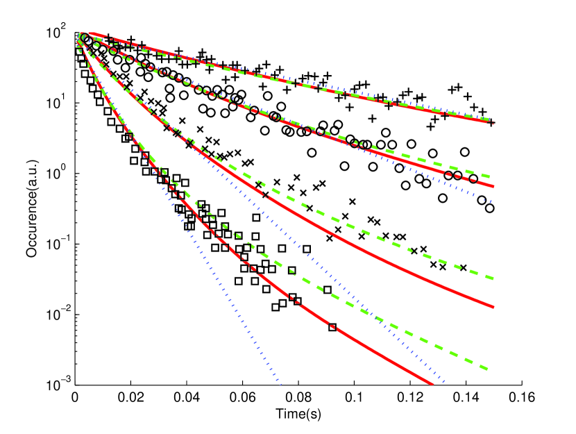
Figure 1: Waiting time distribution vs. substrate concentration. The dotted and dashed lines and the experiment data are from Ref. English . The substrate concentrations are 10 $\mu$M (the cross), 20 $\mu$M (the circle), 50 $\mu$M (the time) and 100 $\mu$M (the square), respectively. The parameters used in Eq. (12) are $k_{1}=5\times 10^{7}M^{-1}s^{-1}$, $k_{-1}=18300$ $s^{-1}$, $a=904$ $s^{-1}$, $b=5.0$ nm and $\sigma=0.1$ nm liufexp .

where $\sigma^{2}=k_{\rm B}T/k$, and $k_{2}(x)=a\exp(-bx)$. It might be the simplest model of Eq. (12). The values of the parameters and fitting results are showed in Fig. 1. We see that our calculation is satisfactory. Because Eq. (12) is almost the same with previous result Kou , we are not ready to explain the general behavior of it afresh. In the following part, we will focus on the general solutions to the coupled diffusion-reaction equations.

Firstly substituting Zusman ; Sumi ; Zhu

$$P_{\rm I}(x,t)=g_{\rm I}(x)Q_{\rm I}(x,t)$$ (15)

into Eq. (Single Molecule Michaelis-Menten Equation beyond Quasi-Static Disorder), where $g_{\rm I}(x)$, I= E, ES, and E⁰ are related to the thermal equilibrium distributions

$$g_{\rm I}(x) = \left[P^{\rm eq}_{\rm I}(x)\right]^{1/2}$$ (16)

$$= e^{-\beta V_{\rm I}(x)/2}\left/\left[\int e^{-\beta V_{\rm I}(x)}dx\right.\right]^{1/2},$$

we transform the diffusion reaction equations into an adjoint form

$$\frac{\partial}{\partial t}Q_{\rm E}(x,t)=-[{\hat{H}}_{\rm E}+k_{1S}(x)]Q_{\rm E}+k_{-1}^{\prime}(x)Q_{\rm ES}$$

$$\frac{\partial}{\partial t}Q_{\rm ES}(x,t)=-[{\hat{H}}_{\rm ES}+k_{3}(x)]Q_{\rm ES}+k_{1S}^{\prime}(x)Q_{\rm E}$$

$$\frac{\partial}{\partial t}Q_{\rm E^{0}}(x,t)=-{\hat{H}}_{\rm E^{0}}Q_{\rm E^{0}}+{k_{2}}^{\prime}(x)Q_{\rm ES},$$ (17)

where the new functions $k_{-1}^{\prime}(x)$, $k_{1S}^{\prime}(x)$ and $k_{2}^{\prime}(x)$ are respectively defined by

$$k_{-1}^{\prime}(x)=k_{-1}^{\prime}g_{\rm ES}/g_{\rm E}(x),$$

$$k_{1S}^{\prime}(x)=k_{1\rm S}g_{\rm E}/g_{\rm ES}(x),$$

$$k_{2}^{\prime}(x)=k_{2}g_{\rm ES}(x)/g_{\rm E^{0}}(x),$$ (18)

and the Hamiltonian operators are

$$H_{\rm I}=-D_{\rm I}\frac{\partial^{2}}{\partial x^{2}}+\frac{\beta D_{\rm I}}{2}\left[\frac{\beta}{2}\left(\frac{dV_{\rm I}}{dx}\right)^{2}-\frac{d^{2}V_{\rm I}}{dx^{2}}\right],$$ (19)

respectively. We assume that the operators ${\hat{H}}_{\rm I}$ have discrete eigenfunctions $|n\rangle_{\rm I}$ (the bound diffusion assumption), $i.e.$,

$${\hat{H}}_{\rm I}|n\rangle_{\rm I}=\epsilon_{{\rm I}_{n}}|n\rangle_{\rm I},\qquad n=0,1,\cdots$$ (20)

then $g_{\rm I}(x)$ are just the lowest order eigenfunctions $|0\rangle_{\rm I}$ in the coordinate representation with zero eigenvalues ($\epsilon_{i_{0}}=0$). The reader is reminded that the diffusion information has been included in the eigenvalues, for instance, given the potentials $V_{\rm I}$ to be harmonic like Eq. (14), then $\epsilon_{{\rm I}_{n}}=nk\beta D_{\rm I}$. Defining ${\hat{O}}_{\rm I}=s+{\hat{H}}_{\rm I}+k_{i}(x)$, here $i=1S$ and 3 respectively correspond to I=E and ES, and ${\hat{O}}_{\rm E^{0}}=s+{\hat{H}}_{\rm E^{0}}$, the Laplace transform solution $Q_{\rm ES}(x,s)$ of Eq. (Single Molecule Michaelis-Menten Equation beyond Quasi-Static Disorder) with the initial conditions can be written as

$$Q_{\rm ES}(x,s)={\hat{O}}_{\rm ES}^{-1}k_{1S}^{\prime}\frac{1}{{\hat{O}}_{\rm E}-k_{-1}^{\prime}{\hat{O}}_{\rm ES}^{-1}k_{1S}^{\prime}}|0\rangle_{\rm E}.$$ (21)

Although the above calculations are exact formally, we cannot say more the inverse operator $\hat{O}_{\rm ES}^{-1}$. Therefore we employ the decoupled approximation Sumi ; Zhu

$$1\approx{k^{j}_{{\rm I}_{\rm eq}}}^{-1}|0\rangle_{\rm I}{}_{\rm I}\langle 0|k_{j},$$ (22)

where $k^{j}_{{\rm I}_{\rm eq}}={}_{\rm I}\langle 0|k_{j}|0\rangle_{\rm I}$. This is would be exact when the expectation value of the operator Eq. (22) is computed in the state $|0\rangle_{\rm I}$. Using the approximated unit operators in Eq. (5) repeatedly, we finally get the analytical form of $f(s)$ as follows,

$$f(s)=\frac{{}_{\rm E}\langle|k_{3}k_{1\rm S}|0\rangle_{\rm E}k^{2}_{{\rm ES}_{\rm eq}}/k^{3}_{{\rm ES}_{\rm eq}}}{s^{2}\left[1+a^{3}_{\rm ES}(s)\right]\left[1+a^{1\rm S}_{\rm E}(s)\right]-{}_{\rm E}\langle 0|k_{3}k_{1\rm S}|0\rangle_{\rm E}{}_{\rm ES}\langle 0|k_{-1}k_{1\rm S}|0\rangle_{\rm ES}/k^{1\rm S}_{{\rm E}_{\rm eq}}k^{3}_{{\rm ES}_{\rm eq}}}$$ (23)

where

$$a^{i}_{\rm I}(s) = {k^{i}_{{\rm I}_{\rm eq}}}^{-1}{}_{\rm I}\langle 0|k_{i}\left(s+{\hat{H}}_{\rm I}\right)^{-1}|0\rangle_{\rm I}$$

$$= k^{i}_{{\rm I}_{\rm eq}}s^{-1}+{k^{i}_{{\rm I}_{\rm eq}}}^{-1}\sum\limits_{n=1}^{\infty}(s+\epsilon_{{\rm I}_{n}})^{-1}\left|{}_{\rm I}\langle 0|k_{i}|n\rangle_{\rm I}\right|^{2},$$

and $i=1S$ and 3 correspond to I=E and ES, respectively. We immediately see that the waiting time distribution $f(t)$ has a multiexponential behavior, because the denominator of Eq. (23) is a higher order ($\geq 2$) polynomial. For instance, if we truncate the $a^{i}_{\rm I}(s)$ to $n$th, $f(t)$ should be a sum of 2(n+1) exponential decay functions. A remarkable conclusion is that, even if the waiting time distribution function has very complicated multiexponential decay behavior, the reciprocal of the first moment of distribution, $\langle t\rangle=-df(s)/ds\left|{}_{s=0}\right.$ still has a simple MM-like expression,

$$\frac{1}{\langle t\rangle}=\frac{{\cal K}[S]}{[S]+{\cal M}},$$ (25)

where

$${\cal M}=k^{3}_{{\rm ES}_{\rm eq}}/{\cal F},$$

$${\cal K}=k^{3}_{{\rm ES}_{\rm eq}}\left(k^{3}_{{\rm ES}_{\rm eq}}k^{1}_{{\rm E}_{\rm eq}}-{}_{\rm ES}\langle 0|k_{1}k_{-1}|0\rangle_{\rm ES}{}_{\rm E}\langle 0|k_{1}k_{3}|0\rangle_{\rm E}\left/k^{3}_{{\rm ES}_{\rm eq}}k^{1}_{{\rm E}_{\rm eq}}\right.\right)^{2}\left/{\cal F}k^{2}_{{\rm ES}_{\rm eq}}{}_{\rm E}\langle 0|k_{1}k_{3}|0\rangle_{\rm E}\right.,$$

and

$${\cal F}=\left(1+{k^{3}_{{\rm ES}_{\rm eq}}}^{-1}\sum\limits_{n=1}^{\infty}\epsilon^{-1}_{{\rm ES}_{n}}\left|{}_{\rm ES}\langle 0|k_{3}|n\rangle_{\rm ES}\right|^{2}\right)k^{1}_{{\rm E_{\rm eq}}}+{k^{1}_{{\rm E}_{\rm eq}}}^{-1}\sum\limits_{n=1}^{\infty}\epsilon^{-1}_{{\rm E}_{n}}\left|{}_{\rm E}\langle 0|k_{1}|n\rangle_{\rm E}\right|^{2}k^{3}_{{\rm ES}_{\rm eq}}.$$

Here we have separated the substrate concentration $[S]$ from the rate $k_{1S}(x)$. Under the two limiting cases discussed at the beginning, Eq. (Single Molecule Michaelis-Menten Equation beyond Quasi-Static Disorder) is approximated to be Zhu

$$a^{i}_{I}(s){\rm}\approx k^{i}_{{\rm I}_{\rm eq}}s^{-1}\qquad(\textrm{slow reaction limit}),$$

$$a^{i}_{I}(s){\rm}\approx k_{i}(x)s^{-1}\qquad(\textrm{nondiffusion limit}).$$ (26)

Substituting them into Eq (23) and making the Laplace transformation, we obtain the same Eqs (Single Molecule Michaelis-Menten Equation beyond Quasi-Static Disorder) and (10). The general solution hence well recovers the two limiting cases. Because the decoupling approximation Eq. (22) has been proved to be a good approximation Sumi ; Zhu , we conclude that classic MM equation still is a good approximation even in the presence of dynamic disorder with arbitrary characteristics.

There are two main contributions in the present work. Firstly we recover the waiting time distribution $f(t)$ obtained by Xie et al. in quasi-static condition, and given a microscopic interpretation of the weight function used by them. But compared to their complicated algebra calculation and a continuum approximation involved, our approach is very simple and direct. We must point out that the current calculations except fitting to the experiment are independent of specific conformational dynamics. Second, we get general waiting time distribution Eq. (23) with arbitrary dynamic disorder, and prove that the reciprocal of its first moment still follows the classic MM equation. Although this conclusion is based on decoupling approximation, it still is positive because this approximation has been proved to work well in various systems. Moreover, it is beyond the quasi-static disorder condition. While the discrete chemical reaction scheme of Xie et al is hard to achieve because of mathematic difficult. We believe that Eq. (23) would be more useful than Eq. (10) when experiments are performed on various enzyme molecule under a broad range of environmental condition.

This work was supported in part by the National Science Foundation of China and the National Science Foundation under Grant No. PHY99-07949.

References

• (1) L. Michaelis and M.L. Menten, Biochem. Z. 49, 333 (1913).
• (2) H.P Lu, L. Xun and X.S. Xie, Science 282, 1877 (1998).
• (3) X. Zhuang et al., Science 296, 1473 (2002).
• (4) A.M. van Oijen et al., Science 301, 1235 (2003).
• (5) H. Yang et al., Science 302, 262 (2003).
• (6) O. Flomenbom et al., Proc. Natl. Acad. Sci. USA 102, 2368 (2005).
• (7) B.P. English et al., Nature chem. Biol. 2, 87 (2006).
• (8) S.C Kou, B.J. Cherayil, W. Min, B.P. English, and X.S. Xie, J. Phys. Chem. B. 109, 19068 (2005).
• (9) N. Agmon and J.J. Hopfield, J. Chem. Phys. 78, 6947 (1983).
• (10) L.D. Zusman, Chem. Phys. 49, 295 (1980).
• (11) h. Sumi and R.A. Marcus, J. Chem. Phys. 84, 4894 (1986).
• (12) J.J Zhu and J.C. Rasaiah, J. Chem. Phys. 95, 3325 (1991).
• (13) The reader is reminded that we do not know the real dimension of the distance parameters $b$ and $\sigma$ by fitting the existing experimental data. We appoint them to be nm only as a reference.
Refer to caption