Strongly anisotropic roughness in surfaces driven by an oblique particle flux

Abstract

Using field theoretic renormalization, an MBE-type growth process with an obliquely incident influx of atoms is examined. The projection of the beam on the substrate plane selects a “parallel” direction, with rotational invariance restricted to the transverse directions. Depending on the behavior of an effective anisotropic surface tension, a line of second order transitions is identified, as well as a line of potentially first order transitions, joined by a multicritical point. Near the second order transitions and the multicritical point, the surface roughness is strongly anisotropic. Four different roughness exponents are introduced and computed, describing the surface in different directions, in real or momentum space. The results presented challenge an earlier study of the multicritical point.

I Introduction

The fabrication of numerous nanoscale heterostructures requires the controlled deposition of material onto a substrate. A variety of deposition processes are used, depending on desired surface structure and device performance. Molecular beam epitaxy (MBE), involving directed beams of incident atoms, is particularly suitable if lower growth temperatures and precise in situ control and characterization are desired Joyce:1985 . It is an important goal of both theoretical and experimental investigations to gain an understanding of the resulting surface morphology, in terms of its spatial and dynamic height-height correlations, or more specifically, its roughness.

Beyond the obvious implications for nanoscale devices, surface growth problems also constitute an important class of generic nonequilibrium phenomena Krug:1997 . Particles are deposited on the surface and may diffuse around on it. If deposition occurs from a vapor, desorption or bulk defect formation tend to be important processes; in contrast, both mechanisms can often be neglected in MBE (see for example Lagally:1990 ). After an initial transient, a steady state is established which is characterized by time-independent macroscopic properties, provided a suitable reference frame is chosen. Generically, detailed balance is broken by the incident particle flux SiegertPlischke:1992 , so that this steady state cannot be described by a Boltzmann distribution; instead, its statistical properties have to be determined directly from its dynamical evolution. If one is primarily interested in universal, large scale, long time characteristics, the dynamical evolution can often be cast as a Langevin equation which can be analyzed using techniques from renormalized field theory.

Here, we extend a model MarsiliETAL:1996 due to Marsili et al. to describe MBE-type or ballistic deposition processes with oblique particle incidence. Focusing on large scale properties such as surface roughness, we exploit a coarse-grained (continuum) approach. Adopting an idealized description WolfVillain:1990 ; Villain:1991 ; LaiDasSarma:1991 ; Janssen:1996 , particle desorption and bulk defect formation will be neglected so that all (deterministic) surface relaxation processes are mass-conserving, i.e., can be written as the gradients of equilibrium and non-equilibrium currents. Shot noise in the deposition process requires the addition of a stochastic term to the growth equation. Since the particle beam selects a preferred (“parallel”) direction in the substrate plane, the resulting Langevin equation is necessarily anisotropic. The interplay of interatomic interactions and kinetic effects, such as Schwoebel barriers, generates an anisotropic effective surface tension which can become very small or even vanish. Due to the anisotropy, this leads to four different regimes with potentially scale-invariant behaviors. We analyze these four regimes, identify the scale-invariant ones, and compute the associated anisotropic roughness exponents.

Models with oblique particle incidence have been investigated previously. Focusing on vapor-deposited thin films, Meakin and Krug Meakin:1988 ; MeakinKrug:1990 ; MeakinKrug:1992 considered the ballistic deposition of particles under near-grazing incidence. Under these conditions, columnar patterns form which shield parts of the growing surface from incoming particles. The large scale properties of these structures can be characterized in terms of anisotropic scaling exponents, differentiating parallel and transverse directions KrugMeakin:1989 ; MeakinKrug:1992 .

Following Marsili et al.MarsiliETAL:1996 , our model differs from Krug and Meakin’s approach in two important respects. First, surface overhangs and shadowing effects are neglected so that our results are restricted to near-normal incidence. Second, our model is designed for “ideal MBE”-type growth so that it falls outside the Kardar-Parisi-Zhang universality class KardarParisiZhang:1986 for mass non-conserving growth. However, extending the work of Marsili et al MarsiliETAL:1996 , we include a possibly anisotropic effective surface tension and investigate its effects systematically (see further comments in the following section). Due to the anisotropy, this contribution actually consists of two terms, one controlling relaxation parallel and the other transverse to the beam direction, with coupling constants $\tau_{\|}$ and $\tau_{\bot}$, respectively. Depending on which of these two couplings, $\tau_{\|}$ or $\tau_{\bot}$, vanishes first, ripple-like surface structures are expected, aligned transverse to the soft direction. The roughness properties near these two instabilities, characterized respectively by $\tau_{\bot}=0$ while $\tau_{\|}>0$, and $\tau_{\bot}>0$ while $\tau_{\|}=0$, are discussed in this paper for the first time.

The original theory of Marsili et alMarsiliETAL:1996 is recovered only if both couplings, $\tau_{\|}$ and $\tau_{\bot}$, vanish simultaneously. Since the latter requires the careful tuning of two parameters, it is much less likely to be experimentally relevant than either of the other two instabilities in which only a single parameter must be adjusted. Referring all technical details to a separate publication SPJ-Helsinki , we will point out very briefly that the fixed point and the roughness exponents reported in Marsili et alMarsiliETAL:1996 must be significantly revised.

An important aspect discussed in this article is how to translate surface data into roughness exponents, for inherently anisotropic surface models such as the one analyzed here. If we generalize the standard definitions familiar from isotropic problems, we arrive at four different roughness exponents. SchmittmannZia:1995 Two of these characterize real-space scans along and transverse to the beam direction, and the remaining two are needed to describe scattering (i.e. momentum space) data with parallel or transverse momentum transfer. All four are related by simple scaling laws, but possess distinct numerical values. When analyzing experimental data, it is therefore essential to be aware of these subtleties.

The paper is organized as follows. We first present the underlying Langevin equation for a single-valued height field and briefly review the physical origin of its constituents. We then present a careful definition of the roughness exponents, based on height-height correlation functions and their structure factors. Turning to the renormalization group (RG) analysis, we first discuss a simple scaling symmetry of our model which allows us to identify a set of effective coupling constants. The invariance of our model with respect to tilts of the surface is much more powerful. Since this symmetry is continuous, it gives rise to a Ward identity which relates different vertex functions. This simplifies the renormalization procedure considerably. We then present our main results for the scaling properties of correlation and response functions for the four different cases: (o) both $\tau_{\|}$ and $\tau_{\bot}$ are positive; (i) $\tau_{\|}$ remains positive while $\tau_{\bot}$ vanishes; (ii) $\tau_{\|}$ vanishes while $\tau_{\bot}$ remains positive; and finally, (iii) both $\tau_{\|}$ and $\tau_{\bot}$ vanish simultaneously. Roughness and dynamic critical exponents are derived. We conclude with a short summary and a discussion of the experimental evidence.

II The model

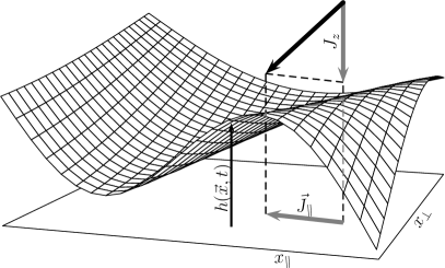
Figure 1: Cartoon of the arrangement of surface and incoming flux. The field $h(\mathbf{x},t)$ is the height of the interface over the substrate. Its coordinate system can always be chosen such that $x_{\parallel}$ is parallel to the projection of the flux on the substrate. The remaining component of the latter is the (negative) flux $J_{z}$.

We focus on long time, large distance phenomena of the growing surface. Under suitable conditions MarsiliETAL:1996 , surface overhangs and shadowing effects may be neglected, so that the surface can be described by a single-valued height field, $h(\mathbf{r},t)$, where $\mathbf{r}$ denotes a $d$-dimensional vector in a reference (substrate) plane, the $z$-axis is normal to that plane, and $t$ denotes time, see Fig. 1. The no-overhang assumption can be justified a posteriori if the calculated interface roughness exponent are found to be less than unity. The time evolution of the interface is described by a Langevin equation of the form

$$\partial_{t}h=G[h]+\eta$$ (1)

Here, $\eta$ denotes the effects of shot noise, and $G[h]$ models the deterministic part of the surface evolution, assumed to be mass-conserving in a suitable coordinate system so that $G[h]$ can be written as a divergence, $G[h]=\mathbf{\nabla\cdot F}[h]$. One contribution to $G[h]$ is due to the incident flux; the other contribution arises from surface diffusion. All of these contributions can be derived using the principle of re-parametrization invariance MarsiliETAL:1996b and are discussed in the following.

As shown in Fig. 1, the incident particle current has a normal component $J_{z}$ and a component parallel to the substrate plane, $\mathbf{J}_{\parallel}$. In the following, the co-ordinate system is rotated such that one of the axes, labelled $x_{\|}$, is aligned with $\mathbf{J}_{\parallel}$. The particles themselves are of finite size with radius $r_{o}$, which implies that the flux responsible for growth at some point on the surface is to be measured at a distance $r$ normal to the surface, see Fig. 2. This effect has been discussed in detail in the literature, see LeamyGilmerDirks:1980 ; MazorETAL:1988 ; MarsiliETAL:1996b . Neglecting higher order terms in the spirit of a gradient expansion, to leading order, this effect gives rise to a deterministic term of the form

$$G_{\mathrm{drive}}[h]=-J_{z}+\mathbf{J}_{\parallel}\cdot\mathbf{\nabla}h+r_{o}J_{z}\nabla^{2}h-r_{o}\left(\mathbf{J}_{\parallel}\cdot\mathbf{\nabla}h\right)\nabla^{2}h$$ (2)

Most remarkably, so called “steering” leads to the same terms in leading order Krug:2005 . Steering implies that deposited atoms are deflected towards the surface normal as soon as they reach a certain distance above it, due to an attractive force exerted by the particles in the deposit. Returning to Eq. (2), we note that the first two terms in $G_{\mathrm{drive}}[h]$ can be removed by a Galilei transformation $h(\mathbf{r},t)\rightarrow h(\mathbf{r+J}_{\parallel}t,t)-J_{z}t$. From now on, we always work in this co-moving frame.

Figure 2: Schematic representation of the growth inhibition and amplification by either finite adatom radii ($r_{o}$) or steering. In both cases, the flux contributing to growth at some point on the surface is to be measured a distance $r_{o}$ normal to the surface. The left box shows the reduced effective surface in valleys, the right one the corresponding effect on peaksMazorETAL:1988 ; Krug:2005 .

In addition to being driven by the incident flux, Eq. (2), the surface also relaxes via diffusion along the surface, leading to a quartic term of the form Mullins:1963

$$G_{\text{{relaxation}}}\ =-\mu\nabla^{4}h$$ (3)

In the following, terms of the form $\tau\nabla^{2}h$ play a particularly important role, since they determine which of the various critical regimes can be accessed. Eq. (2) already contains such a term, induced by $J_{z}$, but other contributions of this type are possible, e.g., a negative term from a step edge (Schwoebel) barrier SchwoebelShipsey:1966 ; Schwoebel:1969 ; Villain:1991 or a positive one due to a surface tension. Moreover, even if such a term were initially absent, it would actually be generated under renormalization group transformations and is therefore intrinsically present. In contrast to Marsili et al.MarsiliETAL:1996 , we include it from the very beginning.

It is essential to note that the nonlinear term in Eq. (2),

$$r_{o}\left(\mathbf{J}_{\parallel}\cdot\mathbf{\nabla}h\right)\,\nabla^{2}h\equiv\lambda\left(\partial_{\parallel}h\right)\,\nabla^{2}h$$

introduces an anisotropy into the system which breaks the full rotational symmetry within the $d$-dimensional space of the substrate. As a consequence, there is no reason to expect isotropic coupling constants (such as $\mu$ or $\tau$) for the linear contributions. Instead, any coarse-graining of the microscopic (atomic level) theory is expected to give rise to different couplings (such as $\tau_{\parallel}$ and $\tau_{\perp}$) in the parallel and perpendicular subspaces, and this is indeed confirmed by the renormalization group. If these anisotropies are incorporated into the theory, preserving only rotational invariance in the $(d-1)$-dimensional transverse subspace, the Langevin equation (1) takes the form

$$\gamma^{-1}\partial_{t}h =\tau_{\parallel}\partial_{\parallel}^{2}h+\tau_{\perp}\nabla_{\perp}^{2}h-\mu_{\parallel}\partial_{\parallel}^{4}h-2\mu_{\times}\nabla_{\perp}^{2}\partial_{\parallel}^{2}h$$

$$-\mu_{\perp}(\nabla_{\perp}^{2})^{2}h+\left(\partial_{\parallel}h\right)\,\bigl{(}\lambda_{\parallel}\partial_{\parallel}^{2}h+\lambda_{\perp}\nabla_{\perp}^{2}h\bigr{)}+\eta$$

$$=-\partial_{\parallel}j_{\parallel}-\mathbf{\nabla}_{\perp}\mathbf{j}_{\perp}+\eta$$ (4)

where we have introduced an explicit time scale for convenience. The surface currents are given by

$$j_{\parallel}= -\partial_{\parallel}\bigl{(}\tau_{\parallel}h-\mu_{\parallel}\partial_{\parallel}^{2}h-\mu_{\times}\nabla_{\perp}^{2}h\bigr{)}$$

$$-\frac{\lambda_{\parallel}}{2}\bigl{(}\partial_{\parallel}h\bigr{)}^{2}+\frac{\lambda_{\perp}}{2}\bigl{(}\nabla_{\perp}h\bigr{)}^{2}\,,$$

$$\mathbf{j}_{\perp}= -\nabla_{\perp}\bigl{(}\tau_{\perp}h-\mu_{\perp}\nabla_{\perp}^{2}h-\mu_{\times}\partial_{\parallel}^{2}h\bigr{)}$$

$$-\lambda_{\perp}\bigl{(}\nabla_{\perp}h\bigr{)}\,\bigl{(}\partial_{\parallel}h\bigr{)}\,.$$ (5)

The scalar differential operator $\partial_{\parallel}$ operates only along $x_{\parallel}$ (see Fig. 1), while the vector $\mathbf{\nabla}_{\bot}$ operates in the $(d-1)$ dimensional subspace perpendicular to $x_{\parallel}$. We also note that the nonlinearity now splits into two distinct terms, with couplings $\lambda_{\parallel}$ and $\lambda_{\perp}$, respectively. Finally, the conserved nature of the deterministic surface evolution is displayed explicitly here.

The randomness of particle aggregation on the surface is captured by the non-conserved white noise $\eta(\mathbf{r},t)$ with zero average and second moment

$$\left\langle\eta(\mathbf{r},t)\eta(\mathbf{r}^{\prime},t^{\prime})\right\rangle=2\gamma^{-1}\delta(\mathbf{r}-\mathbf{r}^{\prime})\ \delta(t-t^{\prime})\ .$$ (6)

Eq. (4) forms the basis for the following analysis. Its properties are controlled by the dominant terms in the gradient expansion. To ensure the stability of the linear theory, we require $\mu_{\parallel},\mu_{\perp}>0$, and $\mu_{\times}\geq-(\mu_{\parallel}\mu_{\perp})^{1/2}$. The two couplings $\tau_{\parallel}$ and $\tau_{\perp}$ play the role of critical control parameters. If both are positive, the nonlinearities become irrelevant, and the problem reduces to the well-known Edwards-Wilkinson equation EdwardsWilkinson:1982 . In contrast, if one or both of them vanish, the long time, long distance properties of the theory change dramatically: The surface undergoes an instability and forms characteristic spatial patterns. If just one of the couplings goes soft, these patterns take the form of ripples (similar to corrugated roofing) transverse to the soft direction. If both couplings become negative, the surface develops mounds or “wedding cakes” Krug:1997 . Focusing only on the onset of these instabilities, four different cases emerge whose properties are discussed in the following: (o) the “disordered” phase, corresponding to the linear theory with $\tau_{\parallel}>0$, $\tau_{\perp}>0$; (i) a line of continuous transitions $\tau_{\parallel}>0$, $\tau_{\perp}\rightarrow 0$; (ii) a line of possibly first order transitions $\tau_{\parallel}\rightarrow 0$, $\tau_{\perp}>0$; and (iii) the multicritical (critical end-) point $\tau_{\parallel}\rightarrow 0$, $\tau_{\perp}\rightarrow 0$. Before we turn to any technicalities, however, we first discuss an important physical issue, namely, the definition of appropriate roughness exponents.

III Anisotropic roughness exponents

The roughness of the surface, and the associated roughness exponents, if they exist, are easily measured experimentally. They can be determined from real-space images of the surface or from scattering data in momentum space. Within our theoretical framework, roughness exponents can be extracted from the height-height correlation function,

$$C(\mathbf{r}-\mathbf{r}^{\prime},t-t^{\prime})\equiv\left\langle h(\mathbf{r},t)h(\mathbf{r}^{\prime},t^{\prime})\right\rangle$$ (7)

Since we focus on the steady state in the absence of spatial boundaries, we assume translational invariance in space and time. The spatial Fourier transform of $C$ is the dynamic structure factor,

$$C(\mathbf{q},t)=\int d^{d}r\,C(\mathbf{r},t)\,e^{i\mathbf{q}\cdot\mathbf{r}}\,.$$

In the absence of anisotropies, the asymptotic scaling behavior of Eq. (7) can be written in the form

$$C(\mathbf{r},t)=\left|\mathbf{r}\right|^{2\chi}c(t/\left|\mathbf{r}\right|^{z})$$ (8)

where $\chi$ denotes the roughness exponent and $z$ the dynamic exponent of the surface while $c$ is a universal scaling function. In Fourier space, the behavior of $C(\mathbf{r},t)$ translates into

$$\widetilde{C}(\mathbf{q},t)=\left|\mathbf{q}\right|^{-(d+2\chi)}\widetilde{c}\left(t\left|\mathbf{q}\right|^{z}\right)$$ (9)

In the presence of strong anisotropy, where the scaling of the correlation function depends on the direction, the situation becomes more complex. Anticipating some of the following results, a key finding of the present article is the existence of four different roughness exponents, characterizing the surface along the parallel or transverse directions, in real or in momentum space. While they are directly related by scaling laws, it is essential to realize that they take different numerical values. In the interpretation of actual experimental data, it is therefore important to identify the appropriate member of this set of four exponents in order to compare with theoretical predictions.

In our scaling analysis below, we adopt the conventional exponent definitions from critical dynamics. The exponent $\nu$ controls the divergence of the correlation length, while $\eta$ denotes the anomalous dimension of the height field which appears in all correlation functions. Due to the presence of anisotropy, an additional exponent, i.e., the strong anisotropy exponent $\Delta$, is required to reflect the different scaling of distances or wave vectors in different directions SchmittmannZia:1995 . If $l$ denotes an arbitrary transverse momentum scale, so that $\left|\mathbf{q}_{\bot}\right|\propto l$, we introduce $\Delta$ via $q_{\|}\propto l^{1+\Delta}$. With this definition, one finds that, asymptotically, the structure factor is a generalized homogeneous function of its variables

$$\widetilde{C}(q_{\|},\mathbf{q}_{\bot};t)=l^{-4+\eta}\widetilde{C}(q_{\|}/l^{1+\Delta},\mathbf{q}_{\bot}/l,l^{z}t)$$ (10)

and in real space, the two-point function takes the form

$$C(x_{\|},\mathbf{r}_{\bot};t)=l^{d+\Delta-4+\eta}C(l^{1+\Delta}x_{\|},l\mathbf{r}_{\bot},l^{z}t)$$ (11)

In analogy to Eq. (8) two roughness exponents are defined in real space, $\chi_{\bot}$ and $\chi_{\|}$, via

$$C(0,\mathbf{r}_{\bot};t) \equiv\left|\mathbf{r}_{\bot}\right|^{2\chi_{\bot}}c_{\bot}(t/\left|\mathbf{r}_{\perp}\right|^{z})$$

$$C(x_{\|},\mathbf{0};t) \equiv\left|x_{\|}\right|^{2\chi_{\|}}c_{{}_{\|}}\bigl{(}t/x_{\|}^{z/(1+\Delta)}\bigr{)}$$ (12)

Of course, this is only meaningful if the two scaling functions $c_{\bot}$ and $c_{{}_{\|}}$ approach finite and non-zero constants when their arguments vanish. Under this assumption, the two exponents

$$\chi_{\bot} = \frac{1}{2}\bigl{[}4-\left(d+\Delta\right)-\eta\bigr{]}$$

$$\chi_{\|} = \frac{1}{2}(1+\Delta)^{-1}\bigl{[}4-\left(d+\Delta\right)-\eta\bigr{]}$$ (13)

are read off immediately. In order to define the corresponding exponents in momentum space, $\tilde{\chi}_{\bot}$ and $\tilde{\chi}_{\|}$, we focus on two structure factors which are easily accessible experimentally, especially if we set $t=0$:

$$\widetilde{C}(0,\mathbf{q}_{\bot},t) \equiv\left|\mathbf{q}_{\bot}\right|^{-(d+2\tilde{\chi}_{\bot})}\widetilde{c}_{\bot}\left(t\left|\mathbf{q}_{\bot}\right|^{z}\right)$$

$$\widetilde{C}(q_{\|},\mathbf{0},t) \equiv q_{\|}^{-(d+2\tilde{\chi}_{\|})}\widetilde{c}_{{}_{\|}}\bigl{(}t\,q_{\|}^{z/(1+\Delta)}\bigr{)}$$ (14)

Again, provided the scaling functions $\widetilde{c}_{\bot}$ and $\widetilde{c}_{\|}$ are nonsingular and non-zero in the limit of vanishing argument, one reads off

$$\tilde{\chi}_{\bot} = \frac{1}{2}\bigl{[}4-d-\eta\bigr{]}$$

$$\tilde{\chi}_{\|} = \frac{1}{2}\bigl{[}\frac{4-\eta}{1+\Delta}-d\bigr{]}$$ (15)

The key observation is that $\tilde{\chi}_{\bot}=\chi_{\bot}$ and $\tilde{\chi}_{\|}=\chi_{\|}$ only if the anisotropy exponent $\Delta$ vanishes. Thus, contrary to Eqs. (8) and (9) which are equivalent definitions of the roughness exponent in isotropic systems, the corresponding definitions for anisotropic systems will typically give rise to different exponents.

In the following, we explicitly compute the scaling exponents in the previous expressions, and also confirm the underlying scaling form. To unify the discussion, we first recast the Langevin equation as a dynamic field theory, collect the elements of perturbation theory, and then identify the upper critical dimensions and marginal nonlinearities for the four cases. Our final goal is a systematic derivation of the scaling properties of correlation and response functions.

IV Renormalization group analysis

IV.1 Power counting and mean-field exponents.

In this section, we assemble the basic components of the field-theoretic analysis, leaving technical details to SPJ-Helsinki . The formalism becomes most elegant if we introduce a response field $\tilde{h}(\mathbf{r},t)$ and recast the Langevin equation (4) as a dynamic functional $\mathcal{J}[\tilde{h},h]$, following standard methods Janssen:1976 ; DeDominicis:1976 ; Janssen:1992 :

$$\mathcal{J}[\tilde{h},h]=\gamma\int d^{d}x\,dt\Big{\{}\tilde{h}\Big{[}\gamma^{-1}\partial_{t}h+\partial_{\parallel}j_{\parallel}+\nabla_{\perp}\mathbf{j}_{\perp}\Big{]}-\tilde{h}^{2}\Big{\}}\,.$$ (16)

This has the advantage that both correlation and response functions can be computed as appropriate functional averages, with statistical weight $\exp(-\mathcal{J})$. The analysis can be simplified considerably if we exploit the symmetries of $\mathcal{J}[\tilde{h},h]$, using the explicit forms of the currents, Eq. (5). First, the symmetry $h(\mathbf{r},t)\rightarrow h(\mathbf{r},t)+a$ implies invariance under a coordinate shift in the $z$-direction. Second, the theory is invariant under tilts of the surface by an infinitesimal “angle” $\mathbf{b}$, i.e., $h(\mathbf{r},t)\rightarrow h(\mathbf{r},t)+\mathbf{b}\cdot\mathbf{r}$ provided the tilt is accompanied by a transformation of the couplings, namely, $\tau_{\parallel}\rightarrow\tau_{\parallel}-b_{\|}\lambda_{\parallel}$ and $\tau_{\perp}\rightarrow\tau_{\perp}-b_{\|}\lambda_{\perp}$. Third, particle conservation on the surface leads to invariance under the symmetry transformation $\tilde{h}(\mathbf{r},t)\rightarrow\tilde{h}(\mathbf{r},t)+c$, $h(\mathbf{r},t)\rightarrow h(\mathbf{r},t)+2c\gamma t$. Finally, we have a symmetry under inversion, namely, $h(x_{\|},\mathbf{r}_{\bot},t)\rightarrow-h(-x_{\|},\mathbf{r}_{\bot},t)\,$, $\tilde{h}(x_{\|},\mathbf{r}_{\bot},t)\rightarrow-\tilde{h}(-x_{\|},\mathbf{r}_{\bot},t)\,$. The most important of these symmetries is the tilt invariance. Thanks to the associated Ward-Takahashi identity Amit:1984 ; Zinn-Justin:1996 , the renormalizations of $\tau_{\parallel}$ and $\tau_{\perp}$ can be related to those of $\lambda_{\parallel}$ and $\lambda_{\perp}$, so that some exponent relations will be valid to all orders in perturbation theory SPJ-Helsinki .

Due to the anisotropy, there are two independent length scales. If only parallel lengths are rescaled, via $x_{\parallel}\rightarrow\alpha x_{\parallel}$, the functional remains invariant provided $h\rightarrow\alpha^{-1/2}h$, $\tilde{h}\rightarrow\alpha^{-1/2}\tilde{h}$ and $\mu_{\parallel}\rightarrow\alpha^{4}\mu_{\parallel}$, $\tau_{\parallel}\rightarrow\alpha^{2}\tau_{\parallel}$, $\mu_{\times}\rightarrow\alpha^{2}\mu_{\times}$ while $\lambda_{\parallel}\rightarrow\alpha^{7/2}\lambda_{\parallel}$ and $\lambda_{\perp}\rightarrow\alpha^{3/2}\lambda_{\perp}$. Likewise, if only transverse lengths are rescaled, via $\mathbf{r}_{\perp}\rightarrow\beta\mathbf{r}_{\perp}$, the functional remains invariant provided $h\rightarrow\beta^{-(d-1)/2}h$, $\tilde{h}\rightarrow\beta^{-(d-1)/2}\tilde{h}$ and $\mu_{\perp}\rightarrow\beta^{4}\mu_{\perp}$, $\tau_{\perp}\rightarrow\beta^{2}\tau_{\perp}$, $\mu_{\times}\rightarrow\beta^{2}\mu_{\times}$ while $\lambda_{\parallel}\rightarrow\beta^{(d-1)/2}\lambda_{\parallel}$ and $\lambda_{\perp}\rightarrow\beta^{(d+3)/2}\lambda_{\perp}$. As a result, the theory naturally gives rise to effective expansion parameters which are invariant under these rescalings. The precise forms of these parameters differ slightly for the four cases and will be discussed next.

In addition to these purely spatial rescalings, we can perform a more general dimensional analysis of Eq. (16), involving both spatial and temporal degrees of freedom. It is standard to express it in terms of an external length scale $\kappa^{-1}$. The key to the scaling of different terms in the functional lies in the behavior of the control parameters $\tau_{\parallel}$ and $\tau_{\perp}$. Depending on whether they vanish or remain finite, the Gaussian part of the dynamic functional is dominated by different terms in the (infrared) limit of small momenta and frequencies.

Case o: If both $\tau_{\parallel}$ and $\tau_{\perp}$ are finite and positive, the theory turns out to be purely Gaussian. Quartic derivatives can be neglected in the infrared limit. It is natural to scale both parallel and transverse momenta by $\kappa$, via $\left|\mathbf{q}_{\bot}\right|\propto$ $q_{\parallel}\propto\kappa$. As a result, time scales as $\kappa^{-2}$ and the fields have dimensions $h(\mathbf{r},t)\propto\kappa^{(d-2)/2}$ and $\tilde{h}(\mathbf{r},t)\propto\kappa^{(d+2)/2}$ so that the nonlinear couplings scale as $\lambda_{\parallel}\propto\lambda_{\perp}\propto\kappa^{-d/2}$ and are therefore irrelevant in any dimension $d>0$. The resulting theory is a simple anisotropic generalization of the Edwards-Wilkinson equation EdwardsWilkinson:1982 ,

$$\gamma^{-1}\partial_{t}h=\tau_{\parallel}\partial_{\parallel}^{2}h+\tau_{\perp}\nabla_{\perp}^{2}h+\eta\ .$$

The anisotropies in the quadratic terms affect only nonuniversal amplitudes and can be removed by a simple rescaling, without losing any information of interest. As is well known, the two-point correlation function scales as

$$C(\mathbf{r},t)=\left|\mathbf{r}\right|^{2-d}c(t/\left|\mathbf{r}\right|^{2})$$

from which one immediately reads off the (isotropic) roughness exponent $\chi=(2-d)/2$ and the dynamic exponent $z=2$. Since this case is so familiar (see Krug:1997 for a detailed discussion), it does not need to be considered further.

Case i: If $\tau_{\parallel}$ remains finite and positive but $\tau_{\perp}$ vanishes, the two leading (Gaussian) terms in the dynamic functional are $\mu_{\perp}\tilde{h}(\nabla_{\perp}^{2})^{2}h$ and $\tau_{\parallel}\tilde{h}\partial_{\parallel}^{2}h$. This suggests that parallel and transverse momenta scale differently, already at the Gaussian level, namely, $\left|\mathbf{q}_{\bot}\right|\propto\kappa$ and $q_{\parallel}\propto\kappa^{2}$. If we rewrite the scaling of parallel momenta as $q_{\parallel}\propto\kappa^{1+\Delta}$, the anisotropic scaling exponent $\Delta$ equals unity for the Gaussian theory. Time scales as $\kappa^{-4}$, and $\tau_{\perp}\propto\kappa^{2}$ is strongly relevant. $\mu_{\perp}$ can be set to $1$ by a transverse rescaling with an appropriate $\beta,$ and $\mu_{\parallel}\propto$ $\mu_{\times}$ $\propto\kappa^{-2}$ are strongly irrelevant (in the renormalization group sense). Introducing the effective dimension $D=d+1$, one finds $h(\mathbf{r},t)\propto\kappa^{(D-4)/2}$ and $\tilde{h}(\mathbf{r},t)\propto\kappa^{(D+4)/2}$. For the nonlinear couplings, we obtain $\lambda_{\perp}\propto\kappa^{(4-D)/2}$ and $\lambda_{\parallel}\propto\kappa^{-D/2}$. Since $D$ is clearly positive, the coupling $\lambda_{\parallel}$ becomes irrelevant. The upper critical dimension $d_{c}$ for the theory is determined by $\lambda_{\perp}$, via $0=4-D$ which leads to $d_{c}=3$. The invariant dimensionless effective expansion parameter is $\tau_{\parallel}^{-3/4}\lambda_{\perp}\kappa^{(d-3)/2}$ as shown by the rescaling $\lambda_{\perp}\rightarrow\alpha^{3/2}\lambda_{\perp}$, $\tau_{\parallel}\rightarrow\alpha^{2}\tau_{\parallel}$. At the Gaussian level, this case corresponds to a critical line parametrized by $\tau_{\parallel}$. The mean-field values for the roughness exponents are simple: In real space, one has $\chi_{\|}=\left(3-d\right)/4$ and $\chi_{\bot}=\left(3-d\right)/2$ while the momentum space exponents are given by $\tilde{\chi}_{\|}=(2-d)/2$ and $\tilde{\chi}_{\bot}=\left(4-d\right)/2$. While the potentially negative value of $\tilde{\chi}_{\|}$ might appear startling, it is simply a consequence of forcing Eq. (10) into the form of Eq. (14).

Case ii: Here, $\tau_{\perp}$ remains finite while $\tau_{\parallel}$ vanishes. The Gaussian part of the functional is dominated by $\tilde{h}\partial_{\parallel}^{4}h$ and $\tau_{\perp}\tilde{h}\nabla_{\perp}^{2}h$. Again, even at the tree level, parallel and transverse momenta scale differently: now, $q_{\parallel}\propto\kappa$ and $\left|\mathbf{q}_{\bot}\right|\propto\kappa^{1+\Delta}$ with $\Delta=1$. Time scales as $\kappa^{-4}$. The strongly relevant perturbation is $\tau_{\parallel}\propto\kappa^{2}$. One may still write $h(\mathbf{r},t)\propto\kappa^{(D-4)/2}$ and $\tilde{h}(\mathbf{r},t)\propto\kappa^{(D+4)/2}$ but the appropriate effective dimension is now $D\equiv(d-1)(1+\Delta)+1$. The two nonlinearities switch roles so that $\lambda_{\parallel}\propto\kappa^{(6-D)/2}$ and $\lambda_{\perp}\propto\kappa^{-D/2}$. In this case, $\lambda_{\perp}$, $\mu_{\perp}$, and $\mu_{\times}$ are irrelevant while $\lambda_{\parallel}$ becomes marginal at the upper critical dimension $d_{c}=7/2$. The invariant dimensionless effective expansion parameter follows from the rescalings as $\mu_{\parallel}^{-7/8}\tau_{\bot}^{-(d-1)/4}\lambda_{\|}\kappa^{(2d-7)/2}$. Again, it appears as if this case corresponds to a critical line parameterized by $\tau_{\perp}$. However, we will see below that the order of the transition may well become first order once fluctuations are included. We therefore refrain from quoting mean-field roughness exponents here.

Case iii: Finally, we consider the multicritical point where both $\tau_{\perp}$ and $\tau_{\parallel}$ vanish. Both momenta scale identically, as $q_{\parallel}\propto\left|\mathbf{q}_{\bot}\right|\propto\kappa$, so that $\Delta=0$ at the tree level. We choose $\beta$ so that $\mu_{\perp}$ scales to $1$. One obtains $\gamma t\propto$ $\kappa^{-4}$, $\tau_{\parallel}\propto\tau_{\perp}\propto\kappa^{2}$, and $h(\mathbf{r},t)\propto\kappa^{(D-4)/2}$, $\tilde{h}(\mathbf{r},t)\propto\kappa^{(D+4)/2}$, with $D=d$. Both nonlinear couplings, $\lambda_{\parallel}$ and $\lambda_{\perp}$, have the same upper critical dimension $d_{c}=6$. The effective expansion parameters are $w\equiv\mu_{\times}/\sqrt{\mu_{\parallel}}$, $u_{\parallel}\equiv\mu_{\parallel}^{-7/8}\lambda_{\parallel}\kappa^{(d-6)/2}$, and $u_{\perp}\equiv\mu_{\parallel}^{-3/8}\lambda_{\perp}\kappa^{(d-6)/2}$. In this case, the anisotropy exponent $\Delta$ vanishes at the tree level so that, to this approximation, all four roughness exponents are equal, given by $\left(4-d\right)/2$. We will see, however, that this changes already in first order of perturbation theory.

In the following, we compute the scaling properties of correlation and response functions for the physically most interesting case (i) in a one-loop approximation. Our findings for cases (ii) and (iii) are reviewed only briefly, leaving the full technical analysis to SPJ-Helsinki .

IV.2 The one-loop approximation.

We use dimensional regularization combined with minimal subtraction Amit:1984 ; Zinn-Justin:1996 . The basic building blocks of the perturbative analysis are the one-particle irreducible vertex functions $\Gamma_{\tilde{N},N}(\{\mathbf{q},\omega\})$ with $\tilde{N}$ ($N$) $h$ ($\tilde{h}$-) amputated legs. The notation $\{\mathbf{q},\omega\}$ is short-hand for the full momentum- and frequency-dependence of these functions. Focusing on the ultraviolet singularities, only those $\Gamma_{\tilde{N},N}$ with positive engineering dimension need to be considered. Taking into account the symmetries and the momentum-dependence carried by the derivatives on the external legs, the set of naively divergent vertex functions is reduced to $\Gamma_{1,1}$ and $\Gamma_{1,2}$ which are computed to one-loop order. Some technical details are relegated to the Appendix.

IV.2.1 Case i: $\tau_{\perp}\rightarrow 0$ and $\tau_{\parallel}>0$

This is the simplest non-trivial case. Only one parameter, $\tau_{\perp}$, needs to be tuned to access criticality. Since $\lambda_{\|}$ is irrelevant, it may be set to zero. Neglecting all other irrelevant terms as well, the functional simplifies to

$$\mathcal{J}[\tilde{h},h] = \gamma\int d^{d}xdt\ \Big{\{}\tilde{h}\bigl{[}\gamma^{-1}\partial_{t}+(\nabla_{\perp}^{2})^{2}-\tau_{\parallel}\partial_{\parallel}^{2}-\tau_{\perp}\nabla_{\perp}^{2}\bigr{]}h$$ (17)

$$- \tilde{h}^{2}-\lambda_{\perp}\tilde{h}(\partial_{\parallel}h)\nabla_{\perp}^{2}h\Big{\}}\,.$$

Thanks to the momentum dependence of the nonlinear term, $\lambda_{\perp}\tilde{h}(\partial_{\parallel}h)\nabla_{\perp}^{2}h$, all divergences in $\Gamma_{1,1}$ and $\Gamma_{1,2}$ are already logarithmic and appear as simple poles in $\varepsilon\equiv d_{c}-d$. In a minimal subtraction scheme, we focus exclusively on these poles and their amplitudes to extract the renormalizations. Since the nonlinearity is cubic in the field, the expansion is organized in powers of $\lambda_{\perp}^{2}$; i.e., the first correction to the tree level is always quadratic for $\Gamma_{1,1}$ and cubic for $\Gamma_{1,2}$. The tilt invariance leads to a Ward identity connecting $\Gamma_{1,1}$ and $\Gamma_{1,2}$, so that only the divergences in $\Gamma_{1,1}$ need to be computed explicitly. Specifically, the tilt transformation $h(\mathbf{r},t)\rightarrow h(\mathbf{r},t)+\mathbf{b}\cdot\mathbf{r}$, $\tau_{\perp}\rightarrow\tau_{\perp}-b_{\|}\lambda_{\perp}$ shows that the parameter $\mathbf{b}$ renormalizes as the field $h$ itself. Hence, the term $\lambda_{\perp}h$ is renormalized by the same factor as $\tau_{\perp}$.

Considering the perturbative contributions to $\Gamma_{1,1}(\mathbf{q},\omega)$ further, we note that all of them carry external momenta, indicating that the terms $\tilde{h}\partial_{t}h$ and $\gamma\tilde{h}^{2}$ do not acquire any corrections. Moreover, particle conservation in conjunction with invariance under parallel inversion and transverse rotations prevents the emergence of corrections to the $\tau_{\perp}\tilde{h}\nabla_{\perp}^{2}h$ term, at any order in perturbation theory. Hence, we should expect only two nontrivial renormalizations in $\Gamma_{1,1}$, namely those for the field $h$ and for the parameter $\tau_{\parallel}$. Leaving the detailed calculations of the renormalized quantities to the Appendix, we seek an infrared stable fixed point for the effective dimensionless coupling $u$, defined as

$$u\equiv A_{\varepsilon}\tau_{\parallel}^{-3/4}\kappa^{-\varepsilon/2}\lambda_{\perp}$$ (18)

where $A_{\varepsilon}$ is a simple geometric factor, defined in the Appendix. A careful analysis of the flow equations for the renormalized parameters reveals the presence of a single infrared stable fixed point, at

$$u^{\ast}=\pm 4\sqrt{\frac{\varepsilon}{3}}\,\bigl{(}1+O(\varepsilon)\bigr{)}\ ,$$ (19)

where the sign is given by the sign of the initial coupling constant $\lambda_{\perp}$. To obtain the scaling properties of correlation and response functions, we exploit the fact that the bare theory is independent of the external momentum scale $\kappa$. The resulting partial differential equation (the renormalization group equation) and its solution is discussed in the Appendix. It predicts, specifically, the scaling form of the height-height correlation function, $C(\mathbf{r},t)$. Including the critical parameter, $\tau_{\bot}$, in its list of arguments, we find:

$$C(\mathbf{r},t;\tau_{\bot})=l^{d+\Delta-4+\eta}C(l^{1+\Delta}x_{\parallel},l\mathbf{r}_{\perp},l^{z}t;l^{-1/\nu_{\bot}}\tau_{\bot})\,\$$ (20)

where $l$ is an arbitrary flow parameter. This behavior of $C(\mathbf{r},t)$ is clearly a natural anisotropic generalization SchmittmannZia:1995 of the usual scaling form of critical dynamics. Moreover, it is clearly consistent with the anticipated scaling behavior, Eq. (11), especially if we set $\tau_{\bot}=0$. The exponents $\nu_{\bot}$, $\eta$, and $z$ have their usual meanings: $\nu_{\bot}$ controls the scaling of the strongly relevant coupling $\tau_{\bot}$, $\eta$ is the anomalous dimension of the field and controls critical correlation functions, and $z$ is the dynamic exponent, relating spatial and temporal fluctuations at criticality. $\Delta$ is the strong anisotropy exponent introduced in Section III. Exploiting the symmetries of the theory fully (see Appendix), we find that $\nu_{\bot}$, $\eta$, and $z$ are related by scaling laws which are exact (at least within perturbation theory):

$$z=4-\eta\,\qquad\text{and}\qquad 1/\nu_{\bot}=2-\eta\text{ }.$$

Assuming that $u^{\ast}$ remains nonzero at higher orders of perturbation theory, its flow equation gives us another exact scaling law, relating $\Delta$ and $\eta$:

$$\Delta+\eta=2-d/3\,$$

As a consequence, only a single exponent, e.g., $\eta$, has to be computed order by order in perturbation theory. Our one-loop calculation results in

$$\eta=-2\varepsilon/3+O(\varepsilon^{2})\,.$$ (21)

Now, all others follow from exponent identities which are exact, at least as long as there are no non-perturbative corrections.

IV.2.2 Case ii: $\tau_{\parallel}\rightarrow 0$ and $\tau_{\perp}>0$

This is the second non-trivial case. Neglecting irrelevant terms, the dynamic functional simplifies to

$$\mathcal{J}[\tilde{h},h]= \gamma\int d^{d}x\,dt\ \Big{\{}\tilde{h}\Big{[}\gamma^{-1}\partial_{t}+\mu_{\parallel}\partial_{\parallel}^{4}-\tau_{\parallel}\partial_{\parallel}^{2}-\tau_{\perp}\nabla_{\perp}^{2}\Big{]}h$$

$$-\tilde{h}^{2}-\lambda_{\parallel}\tilde{h}(\partial_{\parallel}h)\partial_{\parallel}^{2}h\Big{\}}\,.$$ (22)

and the upper critical dimension is now $d_{c}=7/2$.

Following the same approach as in the previous case, we first seek an infrared stable fixed point. The existence of such a fixed point guarantees that the model exhibits a scale-invariant regime where roughness exponents can be defined. As before, we define a suitable effective coupling $u\propto\mu_{\parallel}^{-7/8}\tau_{\perp}^{-(d-1)/4}\lambda_{\parallel}\kappa^{(2d-7)/2}$ and analyze its flow. In this case, however, we find no stable fixed points corresponding to physically meaningful (i.e., real) values of the coupling $u$, at least to this order in perturbation theory SPJ-Helsinki . The lack of such fixed points often indicates a first order transition, but only a more detailed analysis of the underlying mean-field theory or a careful computational study will resolve this issue.

IV.2.3 Case iii: $\tau_{\parallel}\rightarrow 0$ and $\tau_{\perp}\rightarrow 0$

Finally, we briefly review our results for the multicritical point where both critical parameters vanish simultaneously. This case was previously studied by Marsili et al.MarsiliETAL:1996 , in a momentum shell decimation scheme. In this procedure, a hard momentum cutoff prevents the emergence of ultraviolet divergences in the momentum integrals. However, in theories with strong anisotropy and nonlinearities carrying multiple derivatives, the perturbative corrections depend on how the cutoff is implemented, requiring extreme care. This may explain why we were unable to reproduce the earlier MarsiliETAL:1996 results. In contrast, our findings are easy to check, since our field-theoretic approach does not suffer from these complications.

The full functional, defined by Eqs. (16) and (5), now comes into play. To ensure the stability of the critical theory at the tree level, we demand $\mu_{\parallel}\,q_{\parallel}^{4}+2\mu_{\times}q_{\parallel}^{2}\,\mathbf{q}_{\bot}^{2}+(\mathbf{q}_{\bot}^{2})^{2}\geq 0$. This limits the physical range of $\mu_{\parallel}$ and $\mu_{\times}$ to $\mu_{\parallel}>0$ and $\mu_{\times}>-\sqrt{\mu_{\parallel}}$. To complicate matters further, both nonlinear couplings, $\lambda_{\parallel}$ and $\lambda_{\perp}$, are marginal at the upper critical dimension $d_{c}=6$. While the detailed calculations become more involved, the technical analysis remains straightforward SPJ-Helsinki . In particular, thanks to the Ward identity, all renormalizations can still be obtained from the two-point function, $\Gamma_{1,1}$.

The key results are as follows. Again, we define appropriate effective couplings. One of these,

$$w\equiv\frac{\mu_{\times}}{\sqrt{\mu_{\parallel}}}$$

appears in the propagator and generates $w$-dependent algebraic coefficients in the perturbation expansion. The other two,

$$u_{\|} \equiv C_{\varepsilon}\mu_{\parallel}^{-7/8}(1+w)^{-5/4}\lambda_{\|}\kappa^{(d-6)/2}\,\leavevmode\nobreak\ ,$$

$$u_{\bot} \equiv C_{\varepsilon}\mu_{\parallel}^{-3/8}(1+w)^{-5/4}\lambda_{\bot}\kappa^{(d-6)/2}$$

control the nonlinar terms and are treated order by order in perturbation theory. $C_{\varepsilon}$ just absorbs some common geometric constants. A careful analysis of the flow equations for these three couplings shows SPJ-Helsinki that there is only a single, physically meaningful infrared stable fixed point, given by

$$w^{\ast} = 2\sqrt{\frac{3}{5}}-1+O(\varepsilon)\,,\qquad u_{\bot}^{\ast}=0\,,$$

$$u_{\|}^{\ast} = \pm\sqrt{\frac{7\sqrt{15}+25}{11}\,}\varepsilon^{1/2}+O(\varepsilon^{3/2})\,.$$ (23)

This contradicts earlier resultsMarsiliETAL:1996 where a fixed point with $u_{\bot}^{\ast}\neq 0$ was supposedly found.

Exploiting the symmetries of our theory fully and assuming that $u_{\bot}^{\ast}=0$ remains valid to all orders in perturbation theory SPJ-Helsinki , we can determine the critical exponents associated with this model. Remarkably, we find that only a single exponent must be computed explicitly within the $\varepsilon$-expansion, e.g., $\Delta$. The scaling behavior of the height-height correlation function obeys the general form given in Eq. (20), except that both critical parameters now appear, each with its own scaling exponent, $\nu_{\bot}$ and $\nu_{\|}$, respectively. Again, this confirms the anticipated scaling, Eq. (11). The exponents, however, take different values here, demonstrating that cases (i) and (iii) fall into distinct universality classes. Our one-loop calculation yields

$$\Delta=\frac{23+6\sqrt{15}}{11}\varepsilon+O(\varepsilon^{2})\,$$ (24)

The remaining exponents $\eta$, $z$ and $\nu_{\perp}$ do not acquire any corrections beyond the tree results, so that

$$\eta=0\ ,\qquad z=4\ ,\qquad\nu_{\perp}=\frac{1}{2}$$

to all orders in perturbation theory. The exponent $\nu_{\parallel}$ is related to $\Delta$ through an exact scaling relation, namely,

$$\nu_{\|}=\frac{2}{d-2+3\Delta}\,.$$ (25)

These results are sufficient to evaluate the associated roughness exponents.

V Results for the roughness exponents

To begin with, we recall that the scaling forms of the two-point correlations for cases (i) and (iii) are indeed consistent with Eq. (11). We may therefore immediately express the roughness exponents, Eqs. (13) and (15), in terms of the exponent $\Delta$ and $\eta$ for the two universality classes.

For case (i), characterized by $\tau_{\bot}\rightarrow 0$ at positive $\tau_{\|}$, we found only one independent exponent, namely $\eta=-2\varepsilon/3+O(\varepsilon^{2})$ with $\Delta=2-d/2-\eta$. Writing all four roughness exponents in terms of $\eta$, we arrive at expressions which are exact to all orders in $\varepsilon=d-3$:

$$\chi_{\bot} =1-d/3\, \chi_{\|} =\frac{1-d/3}{3-d/3-\eta}\,$$

$$\tilde{\chi}_{\bot} =(4-d-\eta)/2\, \tilde{\chi}_{\|} =\frac{4-\eta}{3-d/3-\eta}-\frac{d}{2}\,\,.$$

The mean-field values are easily recovered by setting $\varepsilon=0$. The physically most interesting case corresponds to a surface grown on a two-dimensional substrate, i.e., $d=2$ and $\varepsilon=1$. For this situation, one obtains $\chi_{\bot}=1/3$ and $\chi_{\|}=1/9+O(\varepsilon^{2})$ while $\tilde{\chi}_{\|}=-2/9+O(\varepsilon^{2})$ and $\tilde{\chi}_{\bot}=4/3+O(\varepsilon^{2})$. Remarkably, the exponent $\chi_{\bot}=1/3$ is actually exact, at least to all orders in perturbation theory.

At the multicritical point, i.e., case (iii) with $\tau_{\bot}\rightarrow 0,\tau_{\|}\rightarrow 0$, we found $\eta=0$ and a nontrivial $\Delta$. Hence,

$$\chi_{\bot} =\frac{1}{2}[4-(d+\Delta)] \chi_{\|} =\frac{4-(d+\Delta)}{2(1+\Delta)}$$

$$\tilde{\chi}_{\bot} =\frac{1}{2}(4-d) \tilde{\chi}_{\|} =\frac{2}{1+\Delta}-\frac{d}{2}\,.$$

All of them are negative near the upper critical dimension $d_{c}=6$. In order to access the physical ($d=2$) situation, one has to set $\varepsilon=4$ here which gives a huge anisotropy exponent, $\Delta\simeq 16.814$, if one naively uses the one-loop result. While roughness exponents can in principle be calculated, we should not place much confidence in their numerical values. Nevertheless, we still obtain testable predictions for this case, namely, the general scaling form of the height-height correlations as well as the scaling laws relating different exponents.

Needless to say, in the absence of an infrared stable fixed point, the renormalization group gives us no information about possible roughness exponents for case (ii) ($\tau_{\perp}>0$, $\tau_{\parallel}\rightarrow 0$). In fact, if the scenario of a first order transition line applies, the whole concept of scaling exponents would be misplaced.

VI Conclusions

To summarize, we have analyzed the long-time, large distance scaling properties of a surface growing under ideal MBE-type conditions, subject to an incident particle beam tilted away from the surface normal. This selects a particular (“parallel”) direction in the substrate plane, so that the resulting growth equations for the (single-valued) height field are spatially anisotropic. In particular, an effective surface tension becomes anisotropic, contributing the terms $\tau_{\parallel}\partial_{\parallel}^{2}h+\tau_{\bot}\nabla_{\bot}^{2}h$ to the right hand side of the Langevin equation. If both of these parameters, $\tau_{\parallel}$ and $\tau_{\perp}$, are positive, the surface is described by the Edwards-Wilkinson model. However, depending on experimental control parameters such as temperature, incident flux rate and angle, or particle size, either $\tau_{\parallel}$ or $\tau_{\perp}$ or both can vanish, generating significantly different surface properties. Each of these three possibilities leads to a distinct field theory with different upper critical dimension. We find $d_{c}=3$ if $\tau_{\perp}\rightarrow 0$ at finite $\tau_{\parallel}$, $d_{c}=7/2$ if $\tau_{\parallel}\rightarrow 0$ at finite $\tau_{\perp}$, and $d_{c}=6$ if both vanish. Only the first and the third case lead to scale-invariant behavior; the second one may in fact trigger a first-order phase transition whose properties lie outside the scope of our RG techniques. Focusing on the first and third case, we find two distinct, novel surface universality classes. For both, we compute the scaling behavior of the two-point height-height correlation function and carefully extract four different roughness exponents. Two of these characterize the height fluctuations of the surface in real space, scanned either along the parallel or the transverse directions; the remaining two characterize scattering data with momentum transfer either along the parallel or the transverse directions. When analyzing experimental data, care must be taken in identifying the correct exponent.

Clearly, the third case requires the careful tuning of two parameters, $\tau_{\parallel}$ and $\tau_{\perp}$. If we can substantiate the presence of a first-order line for $\tau_{\parallel}\rightarrow 0$ at finite $\tau_{\perp}$, the point $\tau_{\parallel}=\tau_{\perp}=0$ would in fact be a critical endpoint, since it separates a line of second order transitions from a line of first order ones. In order to access it in a typical experiment, at least two control parameters have to be tuned very carefully, making it difficult to observe. For this reason, either the second or the first order lines should be more accessible experimentally. From the RG perspective, even if $\tau_{\parallel}$ is set to zero initially, it will be generated under RG transformations, resulting in a non-zero value; this is not the case for the $\tau_{\perp}\nabla_{\perp}^{2}h$ contribution. In that sense, we believe that the most physically relevant theory (apart from Edwards-Wilkinson behavior) is the one with $\tau_{\parallel}>0$ and $\tau_{\perp}=0$. Amongst our key results for this model are the roughness exponents for real-space surface scans. For the physically most interesting case of a two-dimensional surface, we find $\chi_{\bot}=1/3$ if the fluctuations are measured along the transverse direction, and $\chi_{\|}=1/9+O(\varepsilon^{2})$ for scans along the parallel direction. While the value for $\chi_{\|}$ may be modified by higher-order contributions in perturbation theory, the result for $\chi_{\bot}$ is exact.

Finally, we turn to possible experimental evidence for these exponents. Thin films of vapor-deposited gold on smooth glass surfaces HerrastiETAL:1992 ; SalvarezzaETAL:1992 were previously proposed MarsiliETAL:1996 as possible realizations of our theory. The deposit surfaces were imaged by scanning tunneling microscopy (STM), and their mean-square width was measured as a function of STM scan length, resulting in a roughness exponent of $0.35$ HerrastiETAL:1992 ; SalvarezzaETAL:1992 . The temperature is sufficiently low ($T=298$ K) so that desorption is negligeable. Even at small angles of incidence (between $2^{o}$ and $25^{o}$), the growth is anisotropic. The STM images HerrastiETAL:1992 show some evidence for striped pattern formation, if larger sample areas ($\sim 3\times 10^{3}$ nm on each side) are imaged. It is encouraging that a growth exponent close to 1/3 is observed since this matches our prediction for the transverse direction; unfortunately, there seems to be no evidence for the much smaller exponent ($1/9$) which should control the parallel direction. A final resolution of these issues has to await a more detailed analysis of the experimental data.

Appendix

In the following, some technicalities associated with case (i) are presented. We will switch freely between the $\left(\mathbf{q},t\right)$ and the $\left(\mathbf{q},\omega\right)$ representations, depending on which one is more convenient. We first collect the elements of perturbation theory and then discuss the one-loop corrections. Neglecting all nonlinearities in Eq. (17) allows us to identify the bare propagator, $G_{0}(\mathbf{q},t)\,$, and the bare correlator, $C_{0}(\mathbf{q},t)\,$, via

$$G_{0}(\mathbf{q},t)\,\delta(\mathbf{q}-\mathbf{q}^{\prime}) \equiv \langle h(\mathbf{q},t)\tilde{h}(-\mathbf{q}^{\prime},0)\rangle_{0}$$

$$= \theta(t)\,\exp\bigl{(}-\Gamma(\mathbf{q})\gamma t\bigr{)}\,,$$

$$C_{0}(\mathbf{q},t)\,\delta(\mathbf{q}-\mathbf{q}^{\prime}) \equiv \langle h(\mathbf{q},t)h(-\mathbf{q}^{\prime},0)\rangle_{0}$$ (28)

$$= \Gamma(\mathbf{q})^{-1}G_{0}(\mathbf{q},|\,t|)\,,$$

where

$$\Gamma(\mathbf{q})\equiv\mu_{\parallel}q_{\parallel}^{4}+\tau_{\parallel}q_{\parallel}^{2}+\tau_{\perp}\mathbf{q}_{\bot}^{2}$$

Here, $\langle\cdot\rangle_{0}$ denotes a functional average with Gaussian ($\lambda_{\perp}=0$) weight. The Heaviside function $\theta(t)$ is defined with $\theta(0)=0$. Turning to the interaction terms, it is convenient to rewrite them in a symmetrized form. In Fourier space, the expression for the three-point vertex reads

$$V(\mathbf{q}_{1},\mathbf{q}_{2},\mathbf{q}_{3})\equiv i\gamma\lambda_{\perp}\Big{[}\mathbf{q}_{1\bot}\cdot\bigl{(}q_{2\parallel}\,\mathbf{q}_{3\bot}+\mathbf{q}_{2\bot}\,q_{3\parallel}\bigr{)}-q_{1\parallel}\,\mathbf{q}_{2\bot}\cdot\mathbf{q}_{3\bot}\Big{]}\,$$ (29)

with $\mathbf{q}_{1}+\mathbf{q}_{2}+\mathbf{q}_{3}=0$. The sign convention is such that all momenta attached to a vertex are incoming.

We are using dimensional regularization, so that ultraviolet divergences appear as simple poles in $\varepsilon\equiv d_{c}-d$, with $d_{c}=3$. In a minimal subtraction scheme, we focus exclusively on these poles and extract the renormalization constants from their amplitudes. Thanks to the symmetries of the theory, we anticipate only two nontrivial renormalizations, namely those for the field $h$ and for the parameter $\tau_{\parallel}$, both of which can be obtained from $\Gamma_{1,1}$. To one loop order, the explicit expression for the singular part of the two-point vertex function is given by:

$$\Gamma_{1,1}(\mathbf{q},\omega)_{\mathrm{pole}} = i\omega+\gamma\big{[}\tau_{\parallel}q_{\parallel}^{2}+(\mathbf{q}_{\bot}^{2})^{2}+\tau_{\perp}\mathbf{q}_{\bot}^{2}\big{]}$$

$$+ \gamma\frac{u^{2}}{8\varepsilon}\big{[}2\tau_{\parallel}q_{\parallel}^{2}-(\mathbf{q}_{\bot}^{2})^{2}\big{]}+O(u^{4})\,,$$

where the effective expansion parameter $u$ is given by

$$u\equiv A_{\varepsilon}\tau_{\parallel}^{-3/4}\kappa^{-\varepsilon/2}\lambda_{\perp}$$ (31)

and $A_{\varepsilon}$ summarizes a geometric factor which appears in all Feynman diagrams:

$$A_{\varepsilon}\equiv\frac{S_{d-1}}{(2\pi)^{d}}\sqrt{\pi}\Gamma\left(\frac{1-\varepsilon}{2}\right)\Gamma\left(\frac{1+\varepsilon}{2}\right)$$

$S_{d}$ is the surface area of the $d$-dimensional unit sphere.

Keeping in mind that there are only two nontrivial renormalizations to all orders, we introduce renormalized quantities via

$$h\rightarrow\mathring{h} = Z^{1/2}h\quad\,\,\,\,\tilde{h}\rightarrow\mathring{\tilde{h}}=Z^{-1/2}\tilde{h}\quad\gamma\rightarrow\mathring{\gamma}=Z\gamma$$

$$\tau_{\perp}\rightarrow\mathring{\tau}_{\perp} = Z^{-1}\tau_{\perp}\quad\,\tau_{\parallel}\rightarrow\mathring{\tau}_{\parallel}=Z^{-1}Z_{\tau}\tau_{\parallel}$$

$$\lambda_{\perp}\rightarrow\mathring{\lambda}_{\perp} = Z^{-3/2}\lambda_{\perp}$$

The renormalized vertex function $\Gamma_{1,1}$ is defined by demanding that

$$\Gamma_{1,1}(\mathbf{q},\omega,\gamma,\tau_{\perp},\tau_{\parallel},u,\kappa)\equiv\mathring{\Gamma}_{1,1}(\mathbf{q},\omega,\mathring{\gamma},\mathring{\tau}_{\perp},\mathring{\tau}_{\parallel},\mathring{\lambda}_{\perp})$$ (32)

be pole-free. One finds

$$Z =1+\frac{u^{2}}{8\varepsilon}+O(u^{4})\,,$$

$$Z_{\tau} =1-\frac{u^{2}}{4\epsilon}+O(u^{4})\,.$$ (33)

The corresponding Wilson functions are defined as the logarithmic derivatives of the associated $Z$-factors, at constant bare quantities, i.e.,

$$\zeta \equiv \kappa\partial_{\kappa}\ln Z|_{\text{bare}}=-\frac{u^{2}}{8}+O(u^{4})\ ,\qquad$$

$$\zeta_{\tau} \equiv \kappa\partial_{\kappa}\ln Z_{\tau}|_{\text{bare}}=\frac{u^{2}}{4}+O(u^{4})$$ (34)

The flow of the dimensionless effective coupling constant $u$ under renormalization is controlled by the Gell-Mann–Low function,

$$\beta(u) \equiv\kappa\partial_{\kappa}u|_{\text{bare}}=u\big{[}-\frac{\varepsilon}{2}+\frac{3}{4}\left(\zeta+\zeta_{\tau}\right)\big{]}\,$$

$$=u\big{[}-\frac{\varepsilon}{2}+\frac{3}{32}u^{2}+O(u^{4})\big{]}\,.$$ (35)

The renormalization group equation (RGE) for the Green functions, i.e., the connected correlation functions with $N$ ($\tilde{N}$) external $h$ ($\tilde{h}$) legs, simply states that the bare theory is independent of the external momentum scale $\kappa$:

$$0 = \kappa\frac{d}{d\kappa}\mathring{G}_{N,\tilde{N}}(\{\mathbf{r},t\};\mathring{\tau}_{\bot},\mathring{\tau}_{\|},\mathring{\gamma},\mathring{\lambda}_{\perp})$$

$$= \kappa\frac{d}{d\kappa}Z^{(N-\tilde{N})/2}G_{N,\tilde{N}}(\{\mathbf{r},t\};\tau_{\bot},\tau_{\|};u,\gamma,\kappa)\,.$$

In our case, this equation takes the form

$$\Big{[}\kappa\frac{\partial}{\partial\kappa} + \beta\frac{\partial}{\partial u}-\zeta\gamma\frac{\partial}{\partial\gamma}+\zeta\tau_{\perp}\frac{\partial}{\partial\tau_{\perp}}+$$ (36)

$$+ (\zeta-\zeta_{\tau})\tau_{\parallel}\frac{\partial}{\partial\tau_{\parallel}}+\frac{\zeta}{2}(N-\tilde{N})\Big{]}G_{N,\tilde{N}}=0\,.$$

Asymptotic scaling results from this partial differential equation at an infrared stable fixed point that is a solution of $\beta(u^{\ast})=0$ with $\beta^{\prime}(u^{\ast})>0$. The one-loop approximation Eq. (35) leads to the stable fixed point

$$u^{\ast}=\pm 4\sqrt{\frac{\varepsilon}{3}}\,\bigl{(}1+O(\varepsilon)\bigr{)}\ ,$$ (37)

where the sign is given by the sign of the initial coupling constant $\lambda_{\perp}$. Thus, $u^{\ast}$ is non-zero in the $\varepsilon$-expansion, and making the reasonable assumption that this remains true to all orders in perturbaton theory, we find from Eq. (35) the exact relation

$$\zeta^{\ast}+\zeta_{\tau}^{\ast}=\frac{2\varepsilon}{3}$$ (38)

where we have denoted the Wilson $\zeta$-functions, evaluated at the fixed point, by a superscript $\ast$. Eq. (36) can be solved easily at the fixed point $u^{\ast}$, using the method of characteristics, combined with dimensional analysis and the rescaling invariances. If we suppress unnecessary arguments, the solution can be written in the form

$$G_{N,\tilde{N}}(\{\mathbf{r},t\};\tau_{\bot})=l^{\delta_{N,\tilde{N}}}G_{N,\tilde{N}}(\{l^{1+\Delta}x_{\parallel},l\mathbf{r}_{\perp},l^{z}t\};l^{-1/\nu}\tau_{\bot})\,$$

where $l$ is an arbitrary flow parameter. The two critical exponents $\Delta$ and $\eta$ can be expressed in terms of the Wilson functions as

$$\Delta=1+\frac{\zeta_{\tau}^{\ast}-\zeta^{\ast}}{2}\leavevmode\nobreak\ ,\qquad\eta\,=\zeta^{\ast}$$ (39)

while scaling laws give us the remaining exponents $\nu$, $z$, and the overall scaling exponent $\delta_{N,\tilde{N}}$:

$$z = 4-\eta\,,\qquad\qquad 1/\nu=2-\eta\,,$$ (40)

$$\delta_{N,\tilde{N}} = \frac{N}{2}(d+\Delta-4+\eta)+\frac{\tilde{N}}{2}(d+\Delta+4-\eta)$$

Finally, Eq. (38) provides another exact scaling law relating $\Delta$ and $\eta$, provided $u^{\ast}\neq 0$ holds to all orders:

$$\Delta+\eta=2-d/3\,$$

As a consequence, only a single exponent, e.g., $\eta$, has to be computed order by order in perturbation theory, and all others follow from exponent identities.

References

- (1) B.A. Joyce, Rep. Prog. Phys. 48, 1637 (1985).
- (2) J. Krug, Adv. Phys. 46, 139 (1997).
- (3) See, e.g., Kinetics of Ordering and Growth at Surfaces, edited by M. Lagally (Plenum, New York 1990)
- (4) M. Siegert and M. Plischke, Phys. Rev. Lett. 68, 2035 (1992) and J. Phys. (France) I, 3, 1371 (1993).
- (5) M. Marsili, A. Maritan, F. Toigo, and J.R. Banavar, Europhys. Lett. 35, 171 (1996)
- (6) D. E. Wolf and J. Villain, Europhys. Lett. 13, 389 (1990).
- (7) J. Villain, J. Phys. I (France) 1, 19 (1991).
- (8) Z.-W. Lai and S. Das Sarma, Phys. Rev. Lett. 66, 2348 (1991)
- (9) H.K. Janssen, Phys. Rev. Lett. 78, 1082 (1996)
- (10) P. Meakin, Phys. Rev. A 38, 994 (1988)
- (11) P. Meakin and J. Krug, Europhys. Lett. 11, 7 (1990)
- (12) P. Meakin and J. Krug, Phys. Rev. A 46, 3390 (1992)
- (13) J. Krug and P. Meakin, Phys. Rev. A 40, 2064 (1989)
- (14) M. Kardar, G. Parisi, and Y. Zhang, Phys. Rev. Lett. 56, 889 (1986)
- (15) B. Schmittmann, G. Pruessner and H.K. Janssen, to appear in J. Phys. A (2006), Special Issue dedicated to the International Workshop Renormalization Group 2005, Helsinki, Finland.
- (16) This is analogous to the discussion of two-point correlations in driven diffusive systems. See, e.g., B. Schmittmann and R.K.P. Zia, Statistical Mechanics of Driven Diffusive Systems. In: Phase Transitions and Critical Phenomena, Vol. 17, ed. by C. Domb and J.L. Lebowitz (Academic Press, New York 1995).
- (17) M. Marsili, A. Maritan, F. Toigo, and J.R. Banavar, Rev. Mod. Phys. 68, 963 (1996)
- (18) H.J. Leamy, G.H. Gilmer, and A.G. Dirks, in Current Topics in Materials Science, Vol. 6, edited by E. Kaldis (North-Holland, Amsterdam,1980)
- (19) A.D. Mazor, J. Srolovitz, P.S. Hagan, and B.G. Bukiet, Phys. Rev. Lett. 60, 424 (1988)
- (20) J.Krug, in Collective Dynamics of Nonlinear and Disordered Systems, eds. G.Radon, W. Just, and W. Häussler (Springer, Berlin 2005)
- (21) W.W. Mullins, Solid surface morphologies governed by capillarity. In: Metal Surfaces: Structure, Energetics and Kinetics, edited by N.A. Gjostein and W.D. Robertson (Metals Park, Ohio: American Society of Metals 1963)
- (22) R.L. Schwoebel and E.J. Shipsey, J. Appl. Phys. 37, 3682 (1966)
- (23) R.L. Schwoebel, J. Appl. Phys. 40, 614 (1969)
- (24) S.F. Edwards and D.R. Wilkinson, Proc. R. Soc. Lond. A 381, 17
- (25) H.K. Janssen, Z. Phys. B 23, 377 (1976); R. Bausch, H.K. Janssen, and H. Wagner, Z. Phys. B 24, 113 (1976); H.K. Janssen, in Dynamical Critical Phenomena and Related Topics (Lecture Notes in Physics, Vol. 104), edited by C.P. Enz, (Springer, Heidelberg, 1979)
- (26) C. DeDominicis, J. Phys. (France) Colloq. 37, C247 (1976); C. DeDominicis and L. Peliti, Phys. Rev. B 18, 353 (1978)
- (27) H.K. Janssen, in From Phase Transitions to Chaos, edited by G. Györgyi, I. Kondor, L. Sasvári, and T. Tél, (World Scientific, Singapore, 1992)
- (28) D.J. Amit, Field Theory, the Renormalization Group and Critical Phenomena, 2nd revised edition, (World Scientific, Singapore, 1989)
- (29) J.Zinn-Justin, Quantum Field Theory and Critical Phenomena, 3rd edition (Clarendon, Oxford, 1996)
- (30) P. Herrasti, P. Ocón, L. Vasquez, R.C. Salvarezza, J.M. Vara, and A. Arvia, Phys. Rev. A 45, 7440 (1992)
- (31) R.C. Salvarezza, L. Vasquez, P. Herrasti, P. Ocón, J.M. Vara, and A. Arvia, Europhys. Lett. A 45, 7440 (1992)