Field-theoretic description of ionic crystallization in the restricted primitive model

Abstract

Effects of charge-density fluctuations on a phase behavior of the restricted primitive model (RPM) are studied within a field-theoretic formalism. We focus on a $\lambda$-line of continuous transitions between charge-ordered and charge-disordered phases that is observed in several mean-field (MF) theories, but is absent in simulation results. In our study the RPM is reduced to a $\phi^{6}$ theory, and a fluctuation contribution to a grand thermodynamic potential is obtained by generalizing the Brazovskii approach. We find that in a presence of fluctuations the $\lambda$-line disappears. Instead, a fluctuation-induced first-order transition to a charge-ordered phase appears in the same region of a phase diagram, where the liquid – ionic-crystal transition is obtained in simulations. Our results indicate that the charge-ordered phase should be identified with an ionic crystal.

I Introduction

Molten salts, ionic liquids or electrolytes can be described by the restricted primitive model (RPM), where impenetrable hard cores of diameter $\sigma$ carry charges with equal magnitude $e$ stell:95:0 ; fisher:94:0 . In the continuum-space RPM a separation into uniform ion-dilute and ion-dense phases with an associated critical point occurs at low densities, a transition to an ionic crystal of the CsCl type occurs at intermediate densities, and at high densities the fcc crystal is stable stillinger:60:0 . The above phase-behavior was confirmed by recent simulations vega:03:0 . In the last decade a very intensive debate was focused on critical properties of the RPM stell:95:0 ; fisher:94:0 ; levin:02:0 ; kleemeier:99:0 ; wagner:02:0 ; wagner:04:0 ; schroer:06:0 ; kostko:04:0 ; luijten:02:0 ; kim:03:0 ; ciach:00:0 ; patsahan:04:1 ; ciach:06:1 . Phase transitions to crystalline phases drew much less attention smit:96:0 ; barrat:87:0 until very recently bresme:00:0 ; vega:03:0 .

In addition to the phase transitions found in simulations, a line of continuous phase transitions ($\lambda$-line) was found in theoretical studies stillinger:60:0 ; outhwaite:75:0 ; stell:95:0 ; stell:99:0 ; patsahan:03:0 ; patsahan:04:0 ; ciach:00:0 ; ciach:01:1 , except from the mean-spherical (MSA) and related approximations leote:94:0 ; evans:95:0 ; stell:95:0 . Along the $\lambda$-line a decay length of a charge-density correlation function, which exhibits exponentially damped oscillations on the length scale $\sim\sigma$, diverges. In some theories the $\lambda$-line is separated from a first-order transition by a tricritical point (tcp)ciach:00:0 ; ciach:05:0 ; dickman:99:0 ; kobelev:02:0 . In Ref. stillinger:60:0 this line was just rejected as an unphysical solution. Indeed, a location of the $\lambda$-line on a phase diagram depends strongly on a regularization of the Coulomb potential inside the hard core ciach:03:1 ; patsahan:04:0 . This fact may indicate that the $\lambda$-line is an artefact that results from approximations made in different theories caillol:04:0 ; patsahan:04:1 . On the other hand, in Ref. outhwaite:75:0 it was conjectured that a divergent correlation length is a signature of a crystallization. No quantitative arguments supporting the above conjecture were given, however. Thus, a role of the $\lambda$-line in the approximate theories stillinger:60:0 ; outhwaite:75:0 ; stell:95:0 ; stell:99:0 ; patsahan:03:0 ; patsahan:04:0 ; ciach:00:0 ; ciach:01:1 (all of them of a mean-field (MF) type), and its existence in the RPM, remained unclear stell:95:0 ; patsahan:04:1 .

Renewed interest in the whole phase diagram of the RPM, especially in the $\lambda$-line and the tcp, is motivated by recent results obtained for the lattice RPM (LRPM), where positions of ions are restricted to sites of different lattices. On lattices with different symmetries, and/or with a lattice constant $a$ corresponding to different values of $\sigma/a\geq 1$, the ions form different periodic patterns at low temperatures $T$ and/or at high densities $\rho$. Different patterns correspond to different charge-ordered phases. Transitions between the high-temperature, charge-disordered phase and the charge-ordered phases are either continuous or first-order, depending on details of a lattice structure panag:99:0 ; ciach:00:0 ; ciach:01:0 ; ciach:01:1 ; ciach:03:0 ; ciach:04:0 ; ciach:04:1 ; diehl:03:0 ; diehl:05:0 ; diehl:06:0 . In particular, on a simple cubic lattice (sc) with $\sigma/a=1$, only an order-disorder transition to a phase with two oppositely charged sublattices occurs; this transition is continuous for $\rho>\rho_{tc}$, where $\rho_{tc}$ denotes density at the tcp. The phase separation into dilute and dense, uniform phases is only metastable stell:99:0 ; dickman:99:0 ; ciach:00:0 ; kobelev:02:0 . Note that no continuous transition is predicted by the MSA for the LRPM hoye:97:0 , in an obvious disagreament with simulations panag:99:0 ; dickman:99:0 ; diehl:03:0 ; diehl:05:0 and exact theoretical predictions hoye:97:0 . The two types of the charge-ordered – charge-disordered transition are shown in Fig.1. According to recent simulations vega:03:0 , the transition lines between the liquid and the CsCl crystal are very similar to the thick lines shown in Fig.1. Note that in contrast to close-packed crystals, the transition density shows significant dependence on temperature. The above observations raise a question on a relation between the $\lambda$-line in the continuum space and the charge-ordered – charge-disordered transitions on the lattice.

Figure 1: Schematic representation of the order-disorder transition in the LRPM. Thin dashed- and solid lines represent continuous and first-order transitions respectively that were found on the sc lattice with $\sigma/a=1$ panag:99:0 ; dickman:99:0 ; ciach:01:1 ; diehl:03:0 ; diehl:05:0 ; ciach:04:0 . The dashed line is a lattice-analog of the $\lambda$-line. Thick solid lines represent the first-order transition that occurs for $\sigma/a=\sqrt{2},2$ panag:99:0 ; ciach:04:0 ; ciach:04:1 ; ciach:05:0 ; diehl:06:0 . The transition shown by the thin lines can be continuously transformed to the transition shown by the thick lines when additional nearest neighbor repulsion $J$ is present. For small values of $J$ the diagram is shown by the thin lines. When $J$ exceeds a certain value, $J_{0}$, the dashed line splits into two lines that move away when $J$ increases ciach:04:0 ; diehl:05:0 , and the first-order transition that occurs for large values of $J$ is represented by the thick solid lines. According to simulation results vega:03:0 , the shape of the liquid-CsCl crystal two-phase region in continuum-space RPM is similar to that shown by the solid lines. Other transitions that occur in some versions of the LRPM and in the continuum space at low- and at high densities are not shown. $T$ and $\rho$ are in arbitrary units.

In this work we study effects of fluctuations on the $\lambda$-line within the field-theoretic description developed in Ref.ciach:00:0 . On a MF level of this theory the phase diagram for each version of the RPM is the same as on the sc lattice with $\sigma/a=1$ (thin lines in Fig.1). Namely, only the order-disorder transition that is continuous for $\rho>\rho_{tc}$ is present ciach:00:0 ; ciach:01:1 ; ciach:04:0 ; ciach:04:1 . When fluctuations are included within the field-theoretic approch initiated by Brazovskii brazovskii:75:0 , in some lattice systems the order-disorder transition becomes fluctuation-induced first order ciach:03:0 ; ciach:04:0 ; ciach:04:1 (thick lines in Fig.1). The order of the transition agrees with simulation results for all considered cases panag:99:0 ; diehl:03:0 ; diehl:05:0 ; diehl:06:0 . In Ref.ciach:04:0 ; ciach:05:0 arguments were given that in the continuum-space RPM the order-disorder transition becomes fluctuation-induced first order as well.

Except from the order of the considered transition, its location on the phase diagram is of major importace for an identification of the charge-ordered phase. On the MF level of our theory the order-disorder transition occurs at low densities and high temperatures, and the separation into uniform ion-dilute and ion-dense phases is suppresed. Beyond MF, and under the assumption that the order-disorder transition is moved away by fluctuations, the considered field theory ciach:00:0 predicts that for low densities the phase separation into ion-dilute and ion-dense phases occurs. The associated critical point belongs to the Ising universality-class ciach:00:0 ; ciach:05:0 ; ciach:06:1 , in agreement with the earlier theoretical arguments by Stell stell:92:0 ; stell:95:0 , and with recent theory patsahan:04:1 , experiments kleemeier:99:0 ; wiegand:98:0 ; schroer:06:0 and simulations orkoulas:99:0 ; yan:99:0 ; luijten:01:0 ; caillol:02:0 ; luijten:02:0 ; kim:03:0 . It is necessary to verify if the fluctuations may lead to a shift of the phase boundaries of the charge-ordered phase from the phase-space region where the gas-liquid separation takes place, to the phase-space region where the CsCl crystal is stable, to make the field-theoretic arguments in favor of the Ising universality class ciach:00:0 ; ciach:05:0 ; ciach:06:1 complete, and to identify the charge-ordered phase with the CsCl crystal. This is a purpose of our work.

Our work is based on the Brazovskii theory, which turned out to be sucessful in a description of phase transitions and structure of soft-matter systems fredrickson:87:0 ; podneks:96:0 ; levin:92:0 . Analogous theory for hard crystals has not been developed yet. The important common feature of the soft- and ionic crystals is that the periodic ordering is not a result of close packing, but follows directly from interaction potentials, or effective, state-dependent potentials that favour periodic structures for any density. Since the leading physical-mechanism that induces the periodic ordering of soft- and ionic crystals is similar, we expect that the Brazovskii approach is an appropriate description of ionic crystallization.

In sec.2 the field-theoretic description of the RPM is described, our approximations are discussed, and notation is fixed. In sec.3 we derive approximate expressions for the grand potential with the fluctuation-contribution included. The following section is devoted to the results obtained for the order-disorder transition. The last section contains a short summary and a discussion.

II Field-theoretic description of the RPM

Field theory for the RPM that is considered in this work was derived in Refs.ciach:00:0 ; ciach:05:0 ; ciach:04:1 . In this section we summarize the key steps of the derivation, discuss assumptions and approximations, and fix our notation. We consider local deviations from the uniform number- and charge densities, $\eta({\bf x})=\rho^{*}({\bf x})-\rho^{*}_{0}=\rho^{*}_{+}({\bf x})+\rho^{*}_{-}({\bf x})-\rho^{*}_{0}$ and $\phi({\bf x})=\rho^{*}_{+}({\bf x})-\rho^{*}_{-}({\bf x})$ respectively. $\rho^{*}_{+}({\bf x})$ and $\rho^{*}_{-}({\bf x})$ correspond to a local number-density of cations and anions respectively, and $\rho^{*}_{0}$ is the most probable number density of ions. Asterisks indicate that all densities are dimensionless, and the unit volume is $\sigma^{3}$, where $\sigma$ is the core diameter. $\phi$ is the charge density in $e/\sigma^{3}$ units, $e$ is the charge. We focus on systems that are globally charge-neutral,

$$\int_{\bf x}\phi({\bf x})=0,$$ (1)

where in this paper we use the notation $\int_{\bf x}\equiv\int d{\bf x}$. Deviations from equilibrium, uniform distributions of ionic species are thermally excited with the probability density ciach:00:0 ; ciach:06:0 ; ciach:05:0

$$p[\phi,\rho^{*}]=\Xi^{-1}\exp\big{(}-\beta\Omega^{MF}[\phi,\rho^{*}]\big{)},$$ (2)

where $\Xi$ is a normalization constant, and in our theory $\Omega^{MF}$ is approximated by ciach:00:0 ; ciach:05:0 ; ciach:04:1

$$\Omega^{MF}[\phi,\rho^{*}]=F_{h}[\phi,\rho^{*}]+U[\phi]-\mu\int_{\bf x}\rho({\bf x}).$$ (3)

$\mu$ is the chemical potential of the ions, $F_{h}=\int_{\bf x}f_{h}$ is the hard-core reference-system Helmholtz free-energy of the mixture in which the core-diameter $\sigma$ of both components is the same. For the continuum RPM we adopt the Carnahan-Starling (CS) form of $f_{h}$ in the local-density approximation,

$$\beta f_{h}(\rho^{*},\phi)=\frac{\rho^{*}+\phi}{2}\log\Big{(}\frac{\rho^{*}+\phi}{2}\Big{)}+\frac{\rho^{*}-\phi}{2}\log\Bigg{(}\frac{\rho^{*}-\phi}{2}\Bigg{)}-\rho^{*}+\rho^{*}\frac{s(4-3s)}{(1-s)^{2}},$$ (4)

where $\rho^{*}=\eta+\rho^{*}_{0}$, for $\rho^{*}=\rho^{*}_{0}$, the $\Omega^{MF}[0,\rho^{*}]$ assumes a minimum, and $s=\pi\rho^{*}/6$. Finally, the energy in the RPM is given by

$$\beta U[\phi]=\frac{\beta^{*}}{2}\int_{\bf x}\int_{\bf x^{\prime}}\theta(|{\bf x^{\prime}-x}|-1)\frac{\phi({\bf x})\phi({\bf x}^{\prime})}{|{\bf x-x^{\prime}}|}=\frac{\beta^{*}}{2}\int_{\bf k}\tilde{\phi}({\bf k})\tilde{V}(k)\tilde{\phi}(-{\bf k}),$$ (5)

where $\int_{\bf k}\equiv\int d{\bf k}/(2\pi)^{3}$. Contributions to the electrostatic energy coming from overlaping cores are not included in (5). We should note that the regularization of the Coulomb potential for $r<\sigma$ is to some extent arbitrary; in particular, in Refs. patsahan:03:0 ; patsahan:04:0 ; caillol:04:0 different regularizations were chosen. Here and below $x=|{\bf x}|$ is measured in $\sigma$ units. $\beta^{*}=1/T^{*}=\beta e^{2}/(D\sigma)$ is the inverse temperature in standard reduced units; $D$ is the dielectric constant of the solvent. $\tilde{V}(k)=4\pi\cos k/k^{2}$ is the Fourier transform of $V(x)=\theta(x-1)/x$, and $k$ is in $\sigma^{-1}$ units. From the minimum condition for $\Omega^{MF}[\phi,\rho^{*}]$ we obtain the relation between $\rho^{*}_{0}$ and the intensive parameters,

$$\beta\mu=\log\rho_{0}^{*}+\frac{s(8-9s+3s^{2})}{(1-s)^{3}}.$$ (6)

The fields $\phi$ and $\eta$ occur with the probability (2), where the functional $\Omega^{MF}[\phi,\rho^{*}_{0}+\eta]$ consists of a constant term $\Omega^{MF}[0,\rho^{*}_{0}]$ which is irrelevant, and of the term that depends on $\phi$ and $\eta$,

$$\Delta\Omega^{MF}[\phi,\eta]=\Omega^{MF}[\phi,\rho^{*}_{0}+\eta]-\Omega^{MF}[0,\rho^{*}_{0}]\\ =\Omega_{2}[\phi,\eta]+\Omega_{int}[\phi,\eta].$$ (7)

The boundary of stability of $\Delta\Omega^{MF}[\phi,\eta]$ is determined by the Gaussian part,

$$\beta\Omega_{2}=\frac{1}{2}\int\frac{d{\bf k}}{(2\pi)^{3}}\Bigg{[}\tilde{C}_{\phi\phi}^{0}(k)\tilde{\phi}({\bf k})\tilde{\phi}(-{\bf k})+\gamma_{0,2}\tilde{\eta}({\bf k})\tilde{\eta}(-{\bf k})\Bigg{]}$$ (8)

where

$$\tilde{C}_{\phi\phi}^{0}(k)=\rho_{0}^{*-1}+\beta^{*}\tilde{V}(k),$$ (9)

and

$$\gamma_{0,2}=\frac{\partial^{2}\beta f_{h}}{\partial\rho^{*2}}|_{\rho^{*}=\rho^{*}_{0}}=\frac{1+4s+4s^{2}-4s^{3}+s^{4}}{(1-s)^{4}\rho_{0}^{*}},$$ (10)

when the CS reference system is used. The boundary of stability, $\tilde{C}_{\phi\phi}^{0}(k_{b})=0$, occurs along the $\lambda$-line

$$T^{*}=-\tilde{V}(k_{b})\rho^{*}_{0}\approx 1.61\rho^{*}_{0},$$ (11)

where $k_{b}\approx 2.46$ corresponds to the minimum of $\tilde{V}(k)$ ciach:01:1 ; ciach:04:1 ; ciach:05:0 .

The last term in Eq.(7) is local, and can be written as

$$\beta\Omega_{int}[\phi,\eta]=\int_{\bf x}\beta\omega_{int}(\phi({\bf x}),\eta({\bf x})),$$ (12)

with

$$\beta\omega_{int}(\phi,\eta)=\sum_{2m+n>2}\frac{\gamma_{2m,n}}{(2m)!n!}\phi^{2m}\eta^{n},$$ (13)

where $\gamma_{2m,n}$ are appropriate derivatives of $\beta f_{h}$. We consider a truncated form of $\beta\omega_{int}(\phi,\eta)$, because otherwise analytical results for the fluctuation-contribution to the grand potential are not possible. Strictly speaking, the above expansion can be truncated for $\phi\to 0$ and $\eta\to 0$. For given values of $\phi$ and $\eta$, in particular for the results of our calculations in the ordered phase, however, the truncated expansion may be oversimplified, especially for small values of $\rho_{0}^{*}$ and for large amplitudes of the fields.

In the field theory the grand potential and the charge-density correlation function are given by

$$\Omega=-kT\log\Xi,$$ (14)

and

$$\langle\phi({\bf x})\phi({\bf x}^{\prime})\rangle=\Xi^{-1}\int D\eta\int D\phi e^{-\beta\Delta\Omega^{MF}}\phi({\bf x})\phi({\bf x}^{\prime})$$ (15)

respectively, where

$$\Xi=\int D\eta\int D\phi e^{-\beta\Delta\Omega^{MF}}.$$ (16)

In the weighted-field approximation (WF) introduced in Ref.ciach:00:0 , and described in more detail in Refs. ciach:04:1 ; ciach:05:0 ; ciach:06:0 , the field $\eta({\bf x})$ is approximated by its most probable form for each given field $\phi({\bf x})$. Another words, for a given field $\phi({\bf x})$, the field $\eta({\bf x})$ is determined by the minimum of $\beta\Delta\Omega^{MF}[\phi,\eta]$ ($\delta\beta\Delta\Omega^{MF}[\phi,\eta]/\delta\eta=0$), and can be written in the form

$$\eta_{WF}(\phi({\bf x}))=\sum_{n}\frac{a_{n}}{n!}\phi({\bf x})^{2n},$$ (17)

where the coefficient $a_{n}$ is given in terms of $\gamma_{2m,j}$ such that $m+j\leq n+1$ ciach:04:1 . Insertion of $\eta_{WF}(\phi({\bf x}))$ into Eq.(7) leads to simplified forms of Eqs.(16) and (15),

$$\Xi=\int D\phi e^{-\beta{\cal H}_{eff}[\phi]}$$ (18)

and

$$\langle\phi({\bf x})\phi({\bf x}^{\prime})\rangle=\Xi^{-1}\int D\phi e^{-\beta{\cal H}_{eff}[\phi]}\phi({\bf x})\phi({\bf x}^{\prime})$$ (19)

respectively, where

$$\beta{\cal H}_{eff}[\phi]=\frac{1}{2}\int_{\bf x}\int_{\bf x^{\prime}}\phi({\bf x})C_{\phi\phi}^{0}({\bf x}-{\bf x}^{\prime})\phi({\bf x}^{\prime})+\sum_{m=2}^{\infty}\frac{{\cal A}_{2m}}{(2m)!}\int_{\bf x}\phi^{2m}({\bf x}).$$ (20)

The coefficient ${\cal A}_{2m}$ is given in terms of $\gamma_{2k,n}$ such that $k+n\leq m$ ciach:04:1 . For the fluctuation-contribution to the average density we obtain

$$\langle\eta({\bf x})\rangle=\Xi^{-1}\int D\phi\eta_{WF}(\phi({\bf x}))e^{-\beta{\cal H}_{eff}[\phi]}=\sum_{n}\frac{a_{n}}{n!}\langle\phi({\bf x})^{2n}\rangle.$$ (21)

Note that when the expansion in Eq.(20) is truncated at the term $\propto\phi^{2m}$, then in a consistent approximation the expansion in Eq.(21) should be truncated at the term $\propto\langle\phi^{2n}\rangle$ with $n\leq m-1$. Otherwise $a_{n}$ would contain the coefficients $\gamma_{2k,j}$ that in $\beta{\cal H}_{eff}[\phi]$ are not included.

We should mention that on the sc lattice the WF approximation yields quite good results for the locations of the continuous order-disorder transition, and of the tcp ciach:04:1 . In general, for the approximate WF theory we cannot expect exact dependence of the calculated quantities on $\rho^{*}_{0}$.

In this work we shall limit ourselves to the $\phi^{6}$ theory, with ${\cal H}_{eff}$ approximated by ${\cal H}_{WF}$ of the form

$$\beta{\cal H}_{WF}[\phi]=\frac{1}{2}\int_{\bf x}\int_{\bf x^{\prime}}\phi({\bf x})C_{\phi\phi}^{0}({\bf x}-{\bf x}^{\prime})\phi({\bf x}^{\prime})+\frac{{\cal A}_{4}}{4!}\int_{\bf x}\phi^{4}({\bf x})+\frac{{\cal A}_{6}}{6!}\int_{\bf x}\phi^{6}({\bf x}).$$ (22)

The explicit forms of ${\cal A}_{4},{\cal A}_{6}$ in the WF theory are given in Appendix A for the CS reference system. The line of instability of ${\cal H}_{WF}[\phi]$ ($\lambda$-line) is given in Eq.(11). For stability reasons the expansion in Eq.(20) can be truncated at the term $\sim\phi^{2n_{0}}$, if the corresponding couplig constant is ${\cal A}_{2n_{0}}>0$. In the case of the CS reference system we have ${\cal A}_{4}>0$ for $\rho_{0}^{*}>\rho_{tc}^{*}\approx 0.09795$, and ${\cal A}_{4}<0$ for $\rho_{0}^{*}<\rho_{tc}^{*}$. We find ${\cal A}_{6}>0$ outside the density interval $\rho_{tc}^{*}<\rho_{0}^{*}<0.1541$. Negative coupling constants were also found for the RPM in Ref.brilliantov:98:0 . We shall not calculate any quantities for $\rho_{tc}^{*}<\rho_{0}^{*}<0.1541$, where the functional (22) is unstable. Near the above range of densities our results are particularly strongly influenced by the lack of the terms $O(\phi^{8})$, and are less accurate than elsewhere.

Note that $\tilde{C}_{\phi\phi}^{0}(k)$ given in Eq.(9) assumes a minimum for $k=k_{b}>0$, and can be written in the form

$$\tilde{C}_{\phi\phi}^{0}(k)=\beta^{*}\big{(}\tau_{0}+\Delta\tilde{V}(k)\big{)}$$ (23)

where

$$\beta^{*}\tau_{0}=\frac{1}{\rho_{0}^{*}}+\beta^{*}\tilde{V}(k_{b})$$ (24)

and

$$\Delta\tilde{V}(k)=\tilde{V}(k)-\tilde{V}(k_{b})\simeq_{k\to k_{b}}v_{2}(k-k_{b})^{2}+O((k-k_{b})^{3}).$$ (25)

Near the line of instability of ${\cal H}_{WF}$, we have $\beta^{*}\tau_{0}\to 0$ (see Eq.(11)). Because $\tilde{C}_{\phi\phi}^{0}(k)$ assumes a minimum for $k=k_{b}$, the fluctuations $\tilde{\phi}({\bf k})$ with $|{\bf k}|\approx k_{b}$ dominate. If the fluctuations with $k$ significantly different from $k_{b}$ are irrelevant, i.e. for $\tau_{0}\ll v_{2}k_{b}^{2}$ brazovskii:75:0 , the term $O((k-k_{b})^{3})$ in Eq.(25) can be neglected, and

$$\tilde{C}_{\phi\phi}^{0}(k)\approx\beta^{*}\tau_{0}+\beta^{*}v_{2}(k-k_{b})^{2}.$$ (26)

Eqs.(26) and (22) with ${\cal A}_{6}=0$ are of a similar form as in the Brazovskii theory brazovskii:75:0 . In the next section we derive an approximate form for the grand potential in the $\phi^{6}$-theory (Eq.(22) and (26)), by generalizing the Brazovskii approach.

III Construction of the Brazovskii-type approximation for the RPM

In the charge-ordered phase characterized by a charge-density profile that is periodic in space, the fluctuating field can be written in the form

$$\phi({\bf x})=\Phi({\bf x})+\psi({\bf x}),$$ (27)

where

$$\Phi({\bf x})=\langle\phi({\bf x})\rangle$$ (28)

describes the ordered phase with a particular symmetry. In the ordered phase Eq.(16) can be rewritten in the form

$$\Xi=\exp\big{(}-\beta{\cal H}_{eff}[\Phi]\big{)}\int D\psi\exp\big{(}-\beta{\cal H}_{fluc}[\Phi,\psi]\big{)},$$ (29)

where

$${\cal H}_{fluc}[\Phi,\psi]={\cal H}_{eff}[\Phi+\psi]-{\cal H}_{eff}[\Phi].$$ (30)

For the $\phi^{6}$ theory (Eq.(22)) we have

$$\beta{\cal H}_{fluc}[\Phi,\psi]=\frac{1}{2}\int_{\bf x}\int_{\bf x^{\prime}}\psi({\bf x})C_{\phi\phi}^{fluc}({\bf x}-{\bf x}^{\prime})\psi({\bf x}^{\prime})+\int_{\bf x}C_{1}({\bf x})\psi({\bf x})+$$ (31)

$$\frac{1}{3!}\int_{\bf x}C_{3}({\bf x})\psi({\bf x})^{3}+\frac{1}{4!}\int_{\bf x}C_{4}({\bf x})\psi({\bf x})^{4}+\frac{1}{5!}\int_{\bf x}C_{5}({\bf x})\psi({\bf x})^{5}+\frac{{\cal A}_{6}}{6!}\int_{\bf x}\psi({\bf x})^{6},$$

where explicit expressions for $C_{\phi\phi}^{fluc}$ and $C_{i}$ are given in Appendix B.

By inserting Eq.(29) into Eq.(14) we obtain a functional of the charge-density distribution $\Phi({\bf x})$,

$$-\beta\Omega[\Phi({\bf x})]=-\beta{\cal H}_{eff}[\Phi({\bf x})]+\log\Big{[}\int D\psi\exp\Big{(}-\beta{\cal H}_{fluc}[\Phi,\psi]\Big{)}\Big{]}.$$ (32)

The above equation gives the grand potential in a system with the charge density constrained to have the form $\Phi({\bf x})$. For the theory given by the coarse-grained Hamiltonian (20), or by its truncated version (22), this result is exact. For the charge distribution given by $\Phi({\bf x})$, the first term in Eq.(32) can be directly calculated. In order to obtain an approximation for the fluctuation contribution, we rewrite ${\cal H}_{fluc}[\Phi,\psi]$ in the form

$${\cal H}_{fluc}[\Phi,\psi]={\cal H}_{G}[\Phi,\psi]+\Delta{\cal H}[\Phi,\psi]$$ (33)

where ${\cal H}_{G}[\Phi,\psi]$ is the Gaussian contribution,

$${\cal H}_{G}[\Phi,\psi]=\frac{1}{2}\int_{\bf x}\int_{\bf x^{\prime}}\psi({\bf x})C_{\phi\phi}({\bf x}-{\bf x}^{\prime})\psi({\bf x}^{\prime}).$$ (34)

$C_{\phi\phi}({\bf x}-{\bf x}^{\prime})$ is inverse to the exact charge-density correlation function, i.e. in Fourier representation $\tilde{C}_{\phi\phi}(k)=1/\tilde{G}_{\phi\phi}(k)$, where

$$\tilde{G}_{\phi\phi}(k)=\frac{\delta^{2}(\beta\Omega[\Phi])}{\delta\tilde{\Phi}(k)\delta\tilde{\Phi}(-k)}.$$ (35)

Next we make an assumption that $\beta\Delta{\cal H}[\Phi,\psi]$ can be treated as a small perturbation. When such an assumption is valid, we can write

$$\log\Bigg{[}\int D\psi e^{-\beta({\cal H}_{G}+\Delta{\cal H})}\Bigg{]}=\log\Bigg{[}\int D\psi e^{-\beta{\cal H}_{G}}\Big{(}1-\beta\Delta{\cal H}+O[(\beta\Delta{\cal H})^{2}]\Big{)}\Bigg{]}$$ (36)

$$=\log\int D\psi e^{-\beta{\cal H}_{G}}+\log\Big{[}1-\langle\beta\Delta{\cal H}\rangle_{G}+O(\langle\beta\Delta{\cal H}\rangle_{G}^{2})\Big{]},$$ (37)

where $\langle...\rangle_{G}$ denotes averaging with the Boltzmann factor $e^{-\beta{\cal H}_{G}}$. Assuming again that $\langle\beta\Delta{\cal H}\rangle_{G}$ is small, we obtain

$$\beta\Omega[\Phi]=\beta{\cal H}_{eff}[\Phi]-\log\int D\psi e^{-\beta{\cal H}_{G}}+\langle\beta\Delta{\cal H}\rangle_{G}+O(\langle\beta\Delta{\cal H}\rangle_{G}^{2}).$$ (38)

In the uniform phase $\beta\Omega$ is given by the same expression, but with $\Phi=0=\beta{\cal H}_{eff}[0]$.

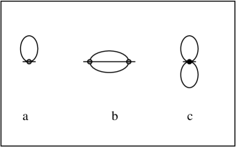
Figure 2: Feynman diagrams contributing to $C_{\phi\phi}$ in the disordered phase, to two-loop order. Shaded circles and a bullet represent ${\cal A}_{4}$ and ${\cal A}_{6}$ respectively. Lines represent $G^{0}_{\phi\phi}$. In the self-consistent theory the lines represent $G^{H}_{\phi\phi}$.

In practice the exact form of $C_{\phi\phi}$ cannot be calculated analytically. In the perturbation theory amit:84:0 ; zinn-justin:89:0 $G_{\phi\phi}$ is given by Feynman diagrams with the $2n$-point vertices ${\cal A}_{2n}$. The vertices at ${\bf x}$ and ${\bf x}^{\prime}$ are connected by lines representing $G^{0}_{\phi\phi}({\bf x}-{\bf x}^{\prime})$, and all lines are paired. The corresponding expressions are integrated over all vertex points, or in Fourier representation over all $\tilde{G}^{0}_{\phi\phi}(k)$-line loops. In this work we shall follow the selfconsistent, one-loop Hartree approximation for $\tilde{C}_{\phi\phi}$ brazovskii:75:0 . The one-loop contribution to $\tilde{C}_{\phi\phi}$ (Fig.2a) is proportional to ${\cal A}_{4}\int_{\bf k}\tilde{G}^{0}_{\phi\phi}(k)$. In the effectively one-loop $\phi^{6}$ theory (22), another contribution to $\tilde{C}_{\phi\phi}(k)$ is given by a diagram (Fig.2c) that is proportional to ${\cal A}_{6}(\int_{\bf k}\tilde{G}^{0}_{\phi\phi}(k))^{2}$ ciach:04:1 ; ciach:05:0 . The symmetry factors of the graphs are calculated according to standared rules amit:84:0 ; zinn-justin:89:0 . In the selfconsistent, effectively one-loop approximation $\tilde{C}_{\phi\phi}(k)$ assumes the approximate form brazovskii:75:0 ; ciach:04:1 ; ciach:05:0

$$\tilde{C}^{H}_{\phi\phi}(k)=r+\beta^{*}\Delta\tilde{V}(k),$$ (39)

where $r\equiv\tilde{C}^{H}_{\phi\phi}(k_{b})$, and by using (35), (31) and (74)-(77) we obtain

$$r=\beta^{*}\tau_{0}+\frac{{\cal A}_{4}{\cal G}(r)}{2}+\frac{{\cal A}_{6}{\cal G}(r)^{2}}{8}+\frac{1}{2}\Big{(}{\cal A}_{4}+\frac{{\cal A}_{6}{\cal G}(r)}{2}\Big{)}\int_{\bf x}\frac{\Phi^{2}({\bf x})}{V}+\frac{{\cal A}_{6}}{4!}\int_{\bf x}\frac{\Phi^{4}({\bf x})}{V}.$$ (40)

In the above $V=\int_{\bf x}1$ is a volume of the system and

$${\cal G}(r)\equiv\langle\psi({\bf x})^{2}\rangle=\int_{\bf k}\tilde{G}^{H}_{\phi\phi}(k).$$ (41)

The remaining diagrams (including the one shown in Fig.2b) are negligible in the $\phi^{4}$ theory for ${\cal A}_{4}\sqrt{\beta^{*}v_{2}}k_{b}\ll r$ brazovskii:75:0 . When the above condition is not satisified, the neglected diagrams, apart from a modification of the form of $r$, yield aditional, $k$-dependent contribution to $\tilde{C}^{H}_{\phi\phi}$ in Eq.(39). Inclusion of such contributions goes beyond the scope of this work.

In general, the integral in Eq.(41) cannot be calculated analytically. In fact the integral diverges because of the integrand behavior for $k\to\infty$. However, the contribution from $k\to\infty$ is unphysical (overlaping hard cores). When the fluctuations with $k\approx k_{b}$ dominate ($r\ll\beta^{*}v_{2}k_{b}^{2}$), then the main physical contribution to ${\cal G}(r)$ comes from $k\approx k_{b}$. In this case the regularized integral is brazovskii:75:0

$${\cal G}(r)=\int_{\bf k}\frac{1}{r+\beta^{*}\Delta\tilde{V}(k)}\simeq_{r\to 0}\int_{\bf k}\frac{1}{r+\beta^{*}v_{2}(k-k_{b})^{2}}=\frac{2a\sqrt{T}^{*}}{\sqrt{r}},$$ (42)

where

$$a=k_{b}^{2}/(4\pi\sqrt{v}_{2}).$$ (43)

The Eqs.(40) and (42) are to be solved selfconsistently for the ordered and the disordered phases. In the disordered phase, i.e. for $\Phi=0$, $r$ is denoted by $r_{0}$.

The second term in Eq.(38), with $\tilde{C}_{\phi\phi}(k)$ approximated by $\tilde{C}^{H}_{\phi\phi}(k)$ (see (39)), is

$$\log\int D\psi e^{-\beta{\cal H}_{G}}\approx-2a\sqrt{T^{*}r}V,$$ (44)

where the approximation (25) and the same regularization as in the case of Eq.(42) were used. For the last term in Eq.(38) we find (see (33), (31), (39) and (40))

$$\langle\beta\Delta{\cal H})\rangle_{G}/V=-\frac{{\cal G}(r)^{2}}{8}{\cal A}_{4}-\frac{{\cal G}(r)^{3}}{24}{\cal A}_{6}-\frac{{\cal G}(r)^{2}}{16}{\cal A}_{6}\int_{\bf x}\frac{\Phi^{2}({\bf x})}{V}.$$ (45)

The above results and Eq.(42) give the explicit form of the grand potential (38)

$$\beta\Omega(\rho_{0}^{*},T^{*};\Phi;r]/V=\beta{\cal H}_{WF}(\rho_{0}^{*},T^{*};\Phi]/V+2a\sqrt{rT^{*}}$$ (46)

$$-\frac{{\cal A}_{4}a^{2}}{2}\frac{T^{*}}{r}-\frac{{\cal A}_{6}a^{3}}{3}\Big{(}\frac{T^{*}}{r}\Big{)}^{3/2}-\frac{{\cal A}_{6}a^{2}}{4}\frac{T^{*}}{r}\int_{\bf x}\frac{\Phi^{2}({\bf x})}{V},$$

where $r=r(\rho_{0}^{*},T^{*};\Phi]$ is a function of $\rho_{0}^{*},T^{*}$ and a functional of $\Phi({\bf x})$ that is to be determined from Eqs. (40) and (42). For given values of $\rho_{0}^{*}$ and $T^{*}$, the value of the (dimensionless) grand potential for a considered phase corresponds to the minimum of $\beta\Omega(\rho_{0}^{*},T^{*};\Phi;r]$ with respect to $\Phi({\bf x})$, with $\rho_{0}^{*}$ and $T^{*}$ fixed.

$T^{*}$ represents temperature, but $\rho_{0}^{*}$ differs from the average number-density when the fluctuations are included (see(21)). The lowest-order fluctuation-induced density shift, given by the first term in Eq.(21), yields the leading contribution to the average local density $\rho^{*}({\bf x})$ of the form

$$\rho^{*}_{1}({\bf x})=\rho^{*}_{0}-\frac{\gamma_{2,1}}{2\gamma_{0,2}}\Big{(}{\cal G}(r)+\Phi({\bf x})^{2}\Big{)}.$$ (47)

The above gives the density shift in the $\phi^{4}$ theory. Higher order terms in Eq.(21) can be included simultaneously with higher-order terms in Eq.(22). In the $\phi^{6}$ theory the next-to-leading order term in Eq.(21) leads to the following approximation for the average density

$$\rho^{*}_{2}({\bf x})=\rho^{*}_{1}({\bf x})+\frac{a_{2}}{2}\Big{[}\Phi({\bf x})^{4}+6\Phi({\bf x})^{2}{\cal G}(r)+3{\cal G}(r)^{2}\Big{]},$$ (48)

where $a_{2}$ is expressed in terms of $\gamma_{2m,n}$ in Appendix A. The thermodynamic density is given by the space-averaged density profile according to

$$\rho^{*}=\int_{\bf x}\frac{\rho^{*}({\bf x})}{V}=\int_{V_{u}}\frac{\rho^{*}({\bf x})}{V_{u}},$$ (49)

where the integration $\int_{V_{u}}$ is over the unit cell of the ordered structure, and $V_{u}$ is the unit-cell volume. Explicit expression for the average density in the liquid is given in Appendix A.

In practice a determination of the equilibrium charge-density profile $\Phi({\bf x})$ and the phase transition between the charge-ordered and charge-disordered phases from Eqs.(46), (40) and (42) is difficult. The problem simplifies greatly when a form of $\Phi({\bf x})$ is limited to a particular function that depends on several parameters. In this case the functionals are reduced to functions of several variables, and the problem of obtaining a minimum of $\beta\Omega$ for a given class of functions becomes tractable.

For an ordered phase of a particular symmetry, $\Phi({\bf x})$ can be written as a linear combination of functions $g_{i}({\bf x})$ forming a corresponding orthonormal basis podneks:96:0 ,

$$\Phi({\bf x})=\sum_{i}\Phi_{i}g_{i}({\bf x}),$$ (50)

where $\Phi_{i}$ are the corresponding amplitudes. In Fourier representation the basis functions can be written in the form

$$\tilde{g}_{i}({\bf k})=\frac{(2\pi)^{d}}{\sqrt{2n_{i}}}\sum_{j=1}^{n_{i}}\Big{(}\delta({\bf k}-{\bf k}^{j}_{ib})+\delta({\bf k}+{\bf k}^{j}_{ib})\Big{)},$$ (51)

where for the considered symmetry $2n_{i}$ and ${\bf k}^{j}_{ib}$ are the number of vectors and the $j$-th vector in the i-th shell respectively. In order to specify the structure we need to know the vectors ${\bf k}^{j}_{ib}$ that determine the size of the unit cell of the structure, apart from the amplitudes $\Phi_{i}$. We assume that the vectors forming the first shell correspond to the wave-vectors of the most probable excitations in the uniform phase. In the theory outlined above such wave-vectors are determined by a minimum of $\tilde{C}_{\phi\phi}(k)$, since it yields a maximum of the probability $\propto\exp(-\beta{\cal H}_{G})$. In the one-loop approximation $\tilde{C}_{\phi\phi}(k)$ assumes a minimum for $|{\bf k}|=k_{b}$, we thus assume $|{\bf k}^{j}_{1b}|=k_{b}$.

When the form of $\Phi({\bf x})$ is restricted to Eq.(50) and $|{\bf k}^{j}_{1b}|=k_{b}$, then for given $\rho^{*}_{0}$ and $T^{*}$, $r=r(\rho_{0}^{*},T^{*};\Phi]$ and $\beta\Omega(\rho_{0}^{*},T^{*};\Phi;r]$ become functions of the amplitudes $\Phi_{i}$. Typically, only the first one- brazovskii:75:0 ; fredrickson:87:0 or two shells podneks:96:0 in Eq.(50) are taken into account in studies of the fluctuation-induced first-order phase transitions brazovskii:75:0 ; fredrickson:87:0 . Our explicit results are obtained in the one-shell approximation,

$$\Phi({\bf x})=\Phi_{1}g_{1}({\bf x}).$$ (52)

For a few points we also considered the two-shell approximation, but the long formulas will not be given here. In the one-shell approximation we can write

$$\int_{\bf x}\frac{\Phi({\bf x})^{2}}{V}=\Phi_{1}^{2},\hskip 28.45274pt\int_{\bf x}\frac{\Phi({\bf x})^{4}}{V}=\Phi_{1}^{4}s_{o},\hskip 28.45274pt\int_{\bf x}\frac{\Phi({\bf x})^{6}}{V}=\Phi_{1}^{6}\kappa_{o},$$ (53)

where

$$s_{o}=\int_{\bf x}\frac{g_{1}({\bf x})^{4}}{V}=\int_{V_{u}}\frac{g_{1}({\bf x})^{4}}{V_{u}}\hskip 28.45274pt\rm{and}\hskip 28.45274pt\kappa_{o}=\int_{\bf x}\frac{g_{1}({\bf x})^{6}}{V}=\int_{V_{u}}\frac{g_{1}({\bf x})^{6}}{V_{u}}$$ (54)

are the geometric factors associated with a particular symmetry of the ordered phase. In the one-shell approximation the above relations should be inserted into Eqs.(40) and (46), and the extremum condition for $\beta\Omega$ can be written in the explicit form

$$r+\Big{(}{\cal A}_{4}+a{\cal A}_{6}\sqrt{\frac{T^{*}}{r}}\Big{)}\Big{(}\frac{s_{o}}{3!}-\frac{1}{2}\Big{)}\Phi_{1}^{2}+\frac{{\cal A}_{6}}{5!}\big{(}\kappa_{o}-5s_{o}\big{)}\Phi_{1}^{4}=0.$$ (55)

The resulting set of equations can be solved for each point $(\rho^{*}_{0},T^{*})$ with respect to $r$ and $\Phi_{1}$. When the results are inserted in Eq.(46), the minimum of the grand-potential is obtained for a given pair of $s_{o}$ and $\kappa_{o}$, i.e. for a chosen structure of the ordered phase. The above method of obtaining the grand potential is equivalent to the method used in Ref.brazovskii:75:0 ; fredrickson:87:0 and outlined in Appendix D. We verified our calculations by comparing the results obtained by both methods.

IV Transition between the charge-ordered and charge-disordered phases

Let us focus on effects of fluctuations on the $\lambda$-line, which on the MF level is given in Eq.(11). At the $\lambda$-line the system becomes unstable with respect to the dominant charge-density fluctuations with the wave number $k_{b}>0$. At the boundary of stability, the second functional-derivative of the grand-potential functional (38) is $\tilde{C}_{\phi\phi}(k_{b})=0$. In the effectively one-loop self-consistent Hartree approximaiton we have $\tilde{C}^{H}_{\phi\phi}(k_{b})=r_{0}$, where $r_{0}$ is a self-consitent solution of Eqs.(40) and (41) with $\Phi=0$. For $r_{0}\ll 1$ the approximation (42) is valid, and we easily find that $r_{0}=0$ is a solution of Eqs.(40) and (42) with $\Phi=0$ only for $T^{*}=0$. Thus, in a presence of fluctuations the $\lambda$-line disappears.

For a given thermodynamic state there may exist one or several minima of $\beta\Omega$ (Eq.(46)), associated with ordered phases with different symmetries. The lowest value of the grand potential for given $\rho^{*}_{0},T^{*}$ corresponds to the stable phase. Other phases are metastable (unstable) if a minimum of the grand potential exists (does not exist). At the phase coexistence two minima of the thermodynamic potential, corresponding to the two coexisting phases, are equal; other minima, if present, are associated with larger values of the grand potential.

When the expansion for $\Phi({\bf x})$ in Eq.(50) is truncated at the first shell, analytical results for the phase coexistence are possible. However, only a very crude approximation for the ordered structure can be obtained. In this study we shall limit ourselves to analytical calculations in the one-shell approximation. More accurate results for the structure of the ordered phase can be obtained numerically in a future work.

We are interested in a stability of the ionic crystal. In the case of the CsCl symmetry ($Pn3m$), the first shell is formed by the three vectors ${\bf k}_{b}^{1}/k_{b}=(1,0,0),{\bf k}_{b}^{2}/k_{b}=(0,1,0)$ and ${\bf k}_{b}^{3}/k_{b}=(0,0,1)$, i.e. $n_{1}=3$, and in real space

$$g^{P}_{1}(x,y,z)=\frac{2}{\sqrt{6}}\Big{(}\cos(k_{b}x)+\cos(k_{b}y)+\cos(k_{b}z)\Big{)}.$$ (56)

The above first shell determines the so called P structure. Unfortunatelly, topological properties of P differ from that of the CsCl crystal. Namely, the P structure is bicontinuous, i.e. the surface $g_{1}({\bf x})=0$ separates space into the positively and negatively charged regions, and both regions are continuous, as shown in Fig.3. In the ionic crystal, however, the positively and negatively charged regions are topologically eqivalent to spheres separated by the uncharged solvent of nonvanishing volume. In addition, the nn distance in the P structure is $\sqrt{3}\pi/k_{b}\approx 2.2$. This distance is much larger than in the actual CsCl crystal. The nn distance in the ionic crystal is closer to the nn distance, $\pi/k_{b}\approx 1.27$, in the case of the one dimensional ordering (lamellar phase), where $n_{1}=1$ and

$$g^{lam}_{1}(x)=\sqrt{2}\cos(k_{b}x).$$ (57)

Since the precise structure of the crystalline phase cannot be determined within the one- or two-shell approximation, we consider both phases to find and compare the transition lines between them and the disordered phase. In this way we gain some insight in the approximate location of the actual phase transition.

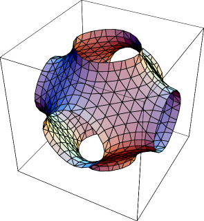
Figure 3: The surface $g_{1}^{P}({\bf x})=0$ in the unit cell of the periodic structure P. This surface separates the positively and negatively charged regions. The lattice constant is $2\pi/k_{b}\approx 2.55$ in ion-diameter units.

IV.1 MF approximation

In the MF the fluctuation contribution to (38) is neglected. In the one-shell approximation the grand potential is a function of the amplitude $\Phi_{1}$,

$$\beta{\cal H}_{WF}(\rho_{0},T^{*},\Phi_{1})/V=\frac{1}{2}\beta^{*}\tau_{0}\Phi_{1}^{2}+\frac{{\cal A}_{4}}{4!}s_{o}\Phi_{1}^{4}+\frac{{\cal A}_{6}}{6!}\kappa_{o}\Phi_{1}^{6},$$ (58)

where the geometric factors $s_{o}$ and $\kappa_{o}$ are found to be

$$s_{o}=\left\{\begin{array}[]{ll}3/2&\;\;\mbox{lamellar structure}\\ 5/2&\;\;\mbox{P structure },\end{array}\right.$$ (61)

and

$$\kappa_{o}=\left\{\begin{array}[]{ll}5/2&\;\;\mbox{lamellar structure}\\ 155/18&\;\;\mbox{P structure }.\end{array}\right.$$ (64)

For $\rho^{*}_{0}>\rho^{*}_{tc}$ the order-disorder transition is continuous and coincides with the line of instability (11), whereas for $\rho^{*}_{0}<\rho^{*}_{tc}$ the order-disorder transition is first order, and occurs when the condition

$$\frac{\partial\beta{\cal H}_{WF}(\rho_{0},T^{*},\Phi_{1})}{\partial\Phi_{1}}=0=\beta{\cal H}_{WF}(\rho_{0},T^{*},\Phi_{1})$$ (65)

is satisfied. The expressions for the transition lines $T^{*}_{lam}$ and $T^{*}_{P}$, and the amplitude $\Phi_{1}$ are given in Appendix C (Eqs.(79) and (80)). It turns out that the P phase is only metastable. However, the relative difference $(T^{*}_{lam}-T^{*}_{P})/T^{*}_{lam}$ is very small.

The density in the ordered phase can be obtained from Eq.(47) by neglecting the fluctuation contribution. In the lowest nontrivial order we have

$$\rho^{*}({\bf x})=\rho^{*}_{0}-\frac{\gamma_{2,1}}{2\gamma_{0,2}}\Phi({\bf x})^{2}.$$ (66)

We verified that Eq.(66) yields $\rho^{*}_{\pm}({\bf x})=(\rho^{*}({\bf x})\pm\Phi({\bf x}))/2\geq 0$ for all space positions. The space-averaged density in the ordered phases is given in Eq.(49). The explicit expression for $\Delta\rho^{*}=\rho^{*}-\rho^{*}_{0}$ is given in Appendix C. The resulting density-temperature phase diagram is shown in Fig.4.

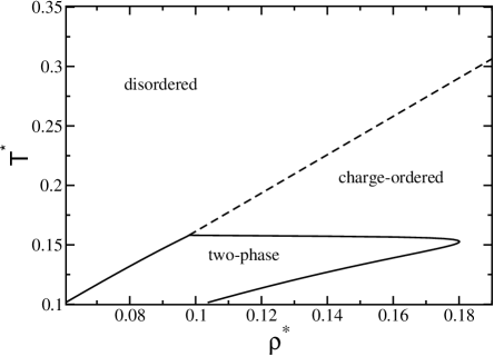
Figure 4: Density-temperature MF phase diagram obtained from the approximate functional (58). Temparature $T^{*}$ and density$\rho^{*}$ are in standard reduced units defined in sec.II.

The diagram shown in Fig.4 is obtained with the functional $\beta\Delta\Omega^{MF}[\phi,\eta]$, Eq.(7), approximated by the functional ${\cal H}_{WF}$, Eq.(22). In order to verify the accuracy of the approximation (22), we calculated the functional $\beta\Delta\Omega^{MF}[\Phi(x),\rho^{*}(x)-\rho^{*}_{0}]$ along the line $T^{*}_{lam}(\rho^{*}_{0})$, for the fields $\Phi(x)$ and $\rho^{*}(x)-\rho^{*}_{0}$ that yield ${\cal H}_{WF}=0$. The result shown in Fig.5 indicates that our approximate functional (22) yields the poorest accuracy in this part of the phase diagram where ${\cal A}_{6}$ is very small (see the discussion below Eqs.(13) and (22)), and the term $\propto\phi^{8}$ should be included. We also considered the two-shell approximation for $\Phi({\bf x})$. We found very similar results, with somewhat lower transition temperatures, and with a smaller difference between them. We conclude that the transition-temperature obtained in the approximate theory (Eq.(22)) is overestimated.

Our main concern in this work is to determine the fluctuation contribution to the grand potential in Eq.(38). We shall not attempt to find better MF results by numerical minimization of the functional (7).

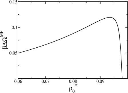
Figure 5: The MF grand potential $\beta\Delta\Omega^{MF}[\Phi({\bf x}),\rho^{*}({\bf x})-\rho^{*}_{0}]$ (see Eq.(7)) along the approximate transition line (79), where ${\cal H}_{WF}=0$. $\Phi({\bf x})$ and $\rho^{*}({\bf x})$ are given in Eq. (52) with (80), and in Eq. (66) respectively.

IV.2 Effects of fluctuations on phase transitions

In this subsection we include the fluctuation contribution to $\Omega$ in Eq.(38).

We consider two cases, the $\phi^{4}$ theory (${\cal A}_{6}\equiv 0$ in the above equations), as in the Brazovskii work brazovskii:75:0 , and the $\phi^{6}$ theory.

IV.2.1 Results of the $\phi^{4}$ theory

The $\phi^{4}$ theory is stable for $\rho^{*}_{0}>\rho^{*}_{tc}$, and for such densities the term $O(\phi^{6})$ can be neglected. In this case analytical solutions for $r_{0}$ and $r$ of Eqs.(40) and (55) can be obtained. Physical solution for $r$ corresponds to the lowest value of $\Phi_{1}$. The transition lines between the uniform and the two ordered phases are shown in Fig.6. In the one-shell approximation the lamellar order turns out to be more stable than the P phase. We also considered the much more tedious two-shell approximation for a few points. We found $\Phi_{2}$ significantly smaller than $\Phi_{1}$, and the phase-transition lines shifted to somewhat lower temperatures compared to the one-shell approximation. The rest of our results is obtained in the much simpler one-shell approximation.

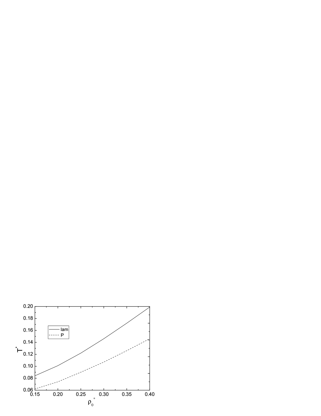
Figure 6: The fluctuation-induced first-order transition lines between the fused salt and the ordered phases in the $\phi^{4}$ theory in the $(\rho_{0}^{*},T^{*})$ phase diagram. The transition to the P phase is metastable.

Recall that our results rely on the approximate Eq.(42), which is valid provided that the condition $r\ll v_{2}k^{2}_{b}/T^{*}(\rho_{0}^{*})$ is satisfied. We verified that along the coexistence lines $T^{*}(\rho_{0}^{*})$ (Fig.6), the $r$ and $r_{0}$ are one and two orders of magnitude smaller than $v_{2}k^{2}_{b}/T^{*}(\rho_{0}^{*})\approx 6/T^{*}(\rho_{0}^{*})$, respectively. Thus, close to the phase coexistence the approximation (42) used in our calculations is valid. However, the condition ${\cal A}_{4}\sqrt{\beta^{*}v_{2}}k_{b}\ll r$, under which the disregarded diagrams (including Fig.2b) can be neglected brazovskii:75:0 is satisfied only for high densities. Therefore the accuracy of our results increases with increasing density.

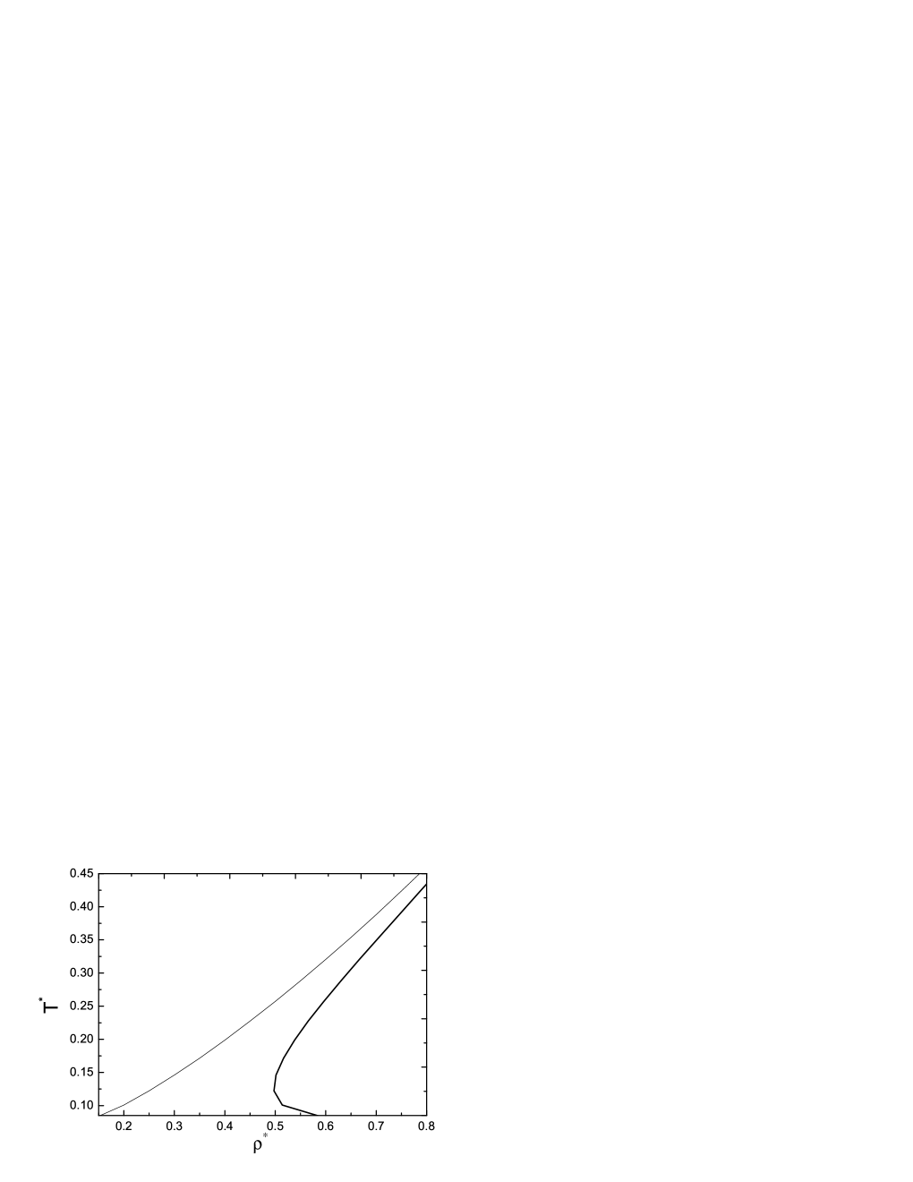
Figure 7: Temperature at the liquid- lamellar phase transition in the $\phi^{4}$ theory as a function of the average density in the liquid phase at different levels of approximation in Eq.(21). Thin solid line corresponds to the zeroth-order term in Eq.(21), i.e. $\rho^{*}$ is approximated by $\rho^{*}_{0}$. Thick solid line is obtained by including the leading-order contribution to the fluctuation-induced density shift, i.e. $\rho^{*}$ is approximated by $\rho^{*}_{1}$ (Eq.(47)). Explicit expression for the average density in the liquid is given Eq.(73).

In Fig.7 the temperature at the transition to the lamellar phase is shown as a function of the most probable density (MF result) and as a function of the average density, given by the approximate expressions (47) and (73). The average density is a nonmonotonic function of $T^{*}$ along the phase coexistence (Fig.7) for $T^{*}<0.15$. As already discussed in sec.3a, for the corresponding range of $\rho^{*}_{0}$ the approximate functional (22) is oversimplified. Moreover, the neglected diagrams (Fig.2b) may yield a relevant contribution to the grand potential for low densities.

Let us compare the temperatures at the continuous transition in MF and at the first-order transition in our theory (Figs.4 and 7). In particular, for $\rho^{*}=0.8$ we find $T^{*}\approx 1.29$ and $T^{*}\approx 0.43$ in the first and in the second case respectively. For $T^{*}\approx 0.43$, on the other hand, we find in MF the transition-density $\rho^{*}_{0}\approx 0.28$, a much lower value than in our theory. As we see, in this approximation the fluctuation-induced shift of the liquid-phase boundary is substantial. However, for $\rho^{*}=0.8$ the temperature at the transition between liquid and the CsCl crystal obtained in simulations  vega:03:0 is $T^{*}\approx 0.1$. Before we identify the charge-ordered phase, we need to find out how the transition temperature and density change when better approximations for ${\cal H}_{WF}$, for the function $\Phi({\bf x})$ and for the average density are made within our theory. In the next section we study the role of the $\phi^{6}$ term in Eq.(22).

IV.2.2 Results of the $\phi^{6}$ theory

In this subsection we determine the effect of the $\phi^{6}$ term on the phase behavior. Analytical solutions for the phase transitions can be obtained by using the original Brazovskii method brazovskii:75:0 ; fredrickson:87:0 , if in equations determining the phase transition the terms of the highest order in $\Phi_{1}$ are neglected. This is justified when $\Phi_{1}\ll 1$. In Appendix D we explain the key steps of the calculations. The full equations in the $\phi^{6}$-theory can only be solved numerically. Results for the transition lines between the uniform and the two ordered phases are shown in Fig.8, where analytical results of the approximate theory and numerical results of the full $\phi^{6}$-theory are shown as lines and as symbols respectively. The liquid-phase boundary, $T^{*}(\rho^{*}_{0})$, is shown in Fig.9 as a function of the average density at different levels of approximation in Eq.(21). The thick solid line is obtained from Eq.(21) with the two leading-order terms included, i.e. in an approximation consistent with Eq.(22). We verified that Eq.(42) used in our calculations is also valid in the $\phi^{6}$-theory.

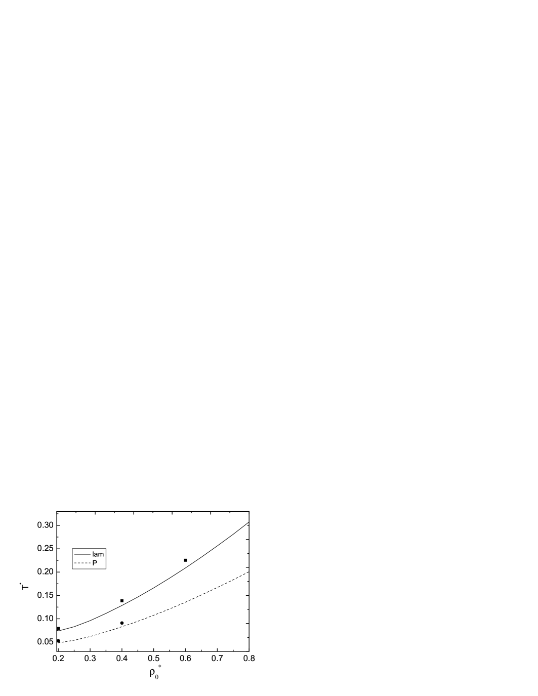
Figure 8: The fluctuation-induced first-order transition lines between the liquid- and the ordered phases in the $\phi^{6}$ theory in the $(\rho_{0}^{*},T^{*})$ phase diagram. Lines are the analytical solutions of the approximate equations (Appendix D) and symbols are the numerical solutions of the full equations described in the text. The transition to the P phase is metastable.

Figure 9: Temperature at the first-order phase transition between liquid and the charge-ordered phase in the $\phi^{6}$ theory, as a function of the average density (21) at different levels of approximation. Thin solid line corresponds to $\rho^{*}$ approximated by the MF result, $\rho^{*}_{0}$. Along the dashed line $\rho^{*}$ is given by the space-averaged leading-order fluctuation-contribution to the average density $\rho^{*}_{1}$ ( Eq.(47)). Thick solid line corresponds to $\rho^{*}_{2}$ ( Eq.(48)), where the next-to-leading orderd term in (21) is taken into account.

By comparing Figs.6 and 8 we see that in the $\phi^{6}$-theory both transition lines are significantly shifted to lower temperatures compared to the $\phi^{4}$-theory. Fig.9 shows that in the consistent approximation for the average density, higher density at the phase coexistence is obtained. The results of the $\phi^{6}$ theory are thus closer to the simulation results for the liquid-CsCl transition, but the transition temperatures are still too high. For example, for $\rho^{*}=0.8$ we have $T^{*}\approx 0.43$ and $T^{*}\approx 0.28$ in the $\phi^{4}$ and in the $\phi^{6}$ theory respectively, whereas for the liquid-CsCl transition $T^{*}\approx 0.1$ for the same density vega:03:0 . Note that the MF results (see the discussion at the end of sec.4a) suggest that the truncated functional (22) leads to overestimated transition temperatures compared to the original functional (7). We can expect that by addition of the term $\sim\phi^{8}$ in Eq.(22) and the third-order term in Eq.(21), lower temperatures and higher densities at the transition should be obtained. Better forms of the charge-density profile $\Phi({\bf x})$ should lead to lower transition-temperatures as well, as indicated by the (partial) results that we obtained in the two-shell approximation. Thus, systematic improvement of the approximations that we make in explicit calculations, should lead to systematically decreasing transition temperature and increasing density, and our results should systematically approach the simulation results for the liquid – ionic-crystal transition vega:03:0 .

For the two quite different charge-ordered phases the transitions to the disordered phase are not far from each other (Fig.8). It is thus plausible that the transitions to the other ordered structures, including the stable one, are located in the same part of the phase diagram.

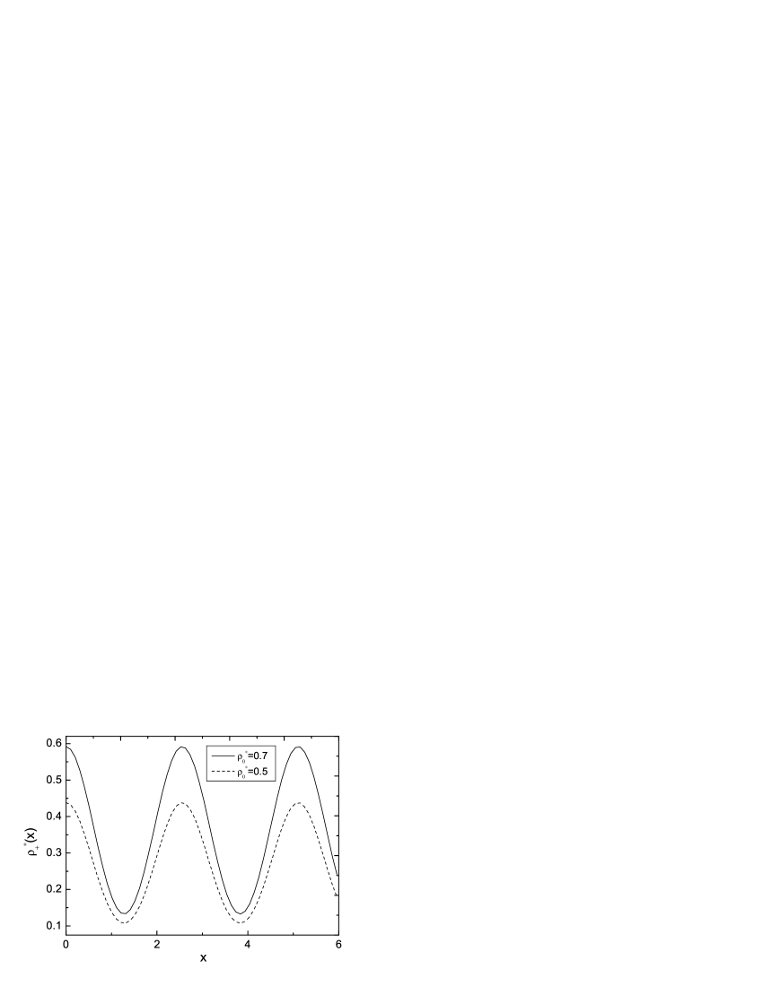
Figure 10: The density profiles of cations, $\rho^{*}_{+}(x)$, in the charge-ordered phase at the coexistence with the liquid phase for two different densities in the $\phi^{6}$ theory. Dashed line corresponds to $\rho_{0}^{*}=0.5$ ($\rho^{*}\approx 0.6$) and the solid line corresponds to $\rho^{*}_{0}=0.7$ ($\rho^{*}\approx 0.75$). $x$ is in $\sigma$-units and $\rho^{*}_{+}$ is dimensionless.

Let us focus on the density difference between the coexisitng phases. In the high-temperature part of the phase coexistence the density difference $\Delta\rho^{*}$ between the coexisting phases is rather small (see Ref.vega:03:0 and Fig.1). By using Eqs.(49) and (48) we find a vanishingly small density difference between the coexisting liquid- and lamellar phases. This result probably follows from the poor, one-shell ansatz for the charge-density profile. The density profile of cations, $\rho^{*}_{+}(x)=(\rho^{*}_{2}(x)+\Phi(x))/2$, where $\rho^{*}_{2}(x)$ is given in Eq.(48), is shown in Fig.10 for two densities at the coexistence with the liquid phase. Beyond the effectively one-loop approximation we expect some (probably weak) dependence of the unit cell of the crystal on density, but its determination requires further studies. The shape of the density profile in the charge-ordered phase resembles an average density profile in a crystal (but only in one direction). Of course in the one-shell approximation the crystalline structure cannot be reproduced accurately. Our results for the liquid phase are more accurate, because they do not depend on the form of $\Phi({\bf x})$, which is the weakest point of our explicit results.

V summary

In this work we considered the fluctuation contribution to the grand-thermodynamic potential in Eq.(32) within the field-theoretic description of the RPM. Our main purpose was a determination of an order, location and nature of the transition between the charge-disordered and charge-ordered phases. We obtained an approximate expression (Eqs.(46), (40) and (42)) for the grand-potential functional of the charge-density profile $\Phi({\bf x})$ in the ordered phase. Our approximation is based on the self-consistent, effectively one-loop Hartree approximation, applied to the $\phi^{6}$ theory that was derived for the RPM in Ref.ciach:04:1 .

We found that in the continuum-space RPM the $\lambda$-line of continuous transitions disappears when the charge-density fluctuations are included. Instead, a first-order transition to a charge-ordered phase appears. The range of temperatures and densities at the first-order transition to the charge-ordered phase is similar to the range of temperatures and densities at the liquid - ionic-crystal transition found in simulations vega:03:0 . In the charge-ordered phase the average charge-density exhibits oscillations with a period $\sim 2.5\sigma$ (beyond the one-loop approximation the period may be slightly different), and with an amplitude $\sim 0.5$. Thus, our results strongly indicate that the fluctuation-induced first-order order-disorder transition should be identified with ionic crystallization. We can conclude that the $\lambda$-line found in different theories of the MF type is in fact a MF indication of ionic crystallization.

The explicit results for the first-order phase transition were obtained analytically within the simplest, one-shell approximation for $\Phi({\bf x})$ (see (52)), for two ordered structures: one-dimensional, lamellar phase, and three-dimansional, P phase shown in Fig.3. We do not expect that the structure of the charge-ordered phase can be correctly reproduced on this simple level of approximation. Our approximate result for the crystalline structure is only a very crude approximation. The transition lines for the two different structures, however, are located close to each other on the $(\rho^{*},T^{*})$ phase diagram. It is thus very plausible that the transition line to the stable phase should be located near the two transition lines, and conclusions concerning the approximate location of the order-disorder transition are justified.

In the effectively one-loop approximation we find the same lattice constant of the CsCl crystal $2\pi/k_{b}$ for a range of densities. Beyond the one-loop approximation we expect a weak dependence of the lattice constant on density. This result and Fig.10 suggest that the number of defects (vacancies) in the crystal coexisitng with the liquid (fused salt) increases with decreasing $T^{*}$. The crystal melts either when at relatively low $T^{*}$ many defects are present (low $\rho^{*}$), or when there are only few defects, but $T^{*}$ is high.

Our results show a reasonable agreement with simulations even for the very crude approximation for $\Phi({\bf x})$, and we verified that by addition of further terms to Eqs.(22), (47) and (52) a better agreement should be obtained. The accuracy of the results can be significantly improved within the approach developed in this work by choosing a better ansatz for the form of $\Phi({\bf x})$. Note that the fluctuation contribution to $\beta\Omega$ depends only on global characteristics of $\Phi({\bf x})$, i.e. on integrals of $\Phi({\bf x})^{2n}$, where $n\leq 3$ in the case of the $\phi^{6}$ theory. Only the MF contribution depends on a detailed shape of $\Phi({\bf x})$ through the term $\int_{\bf x}\int_{\bf x^{\prime}}\Phi({\bf x})C^{0}_{\phi\phi}({\bf x}-{\bf x}^{\prime})\Phi({\bf x}^{\prime})=\int_{\bf k}\tilde{\Phi}({\bf k})\tilde{C}^{0}_{\phi\phi}({\bf k})\tilde{\Phi}({\bf k}^{\prime})$. Numerical determination of the structure of the charge-ordered phase is thus possible within our apporach, but it goes beyond the scope of the present work. We conclude that the field-theoretic approach developed in this work is suitable for a description of ionic crystallization on a semiquantitative level.

VI Appendices

VI.1 Coefficients ${\cal A}_{4},{\cal A}_{6}$ and $a_{2}$ in the WF approximation

The coupling constants in the WF approximation are given in terms of the coefficients $\gamma_{2m,n}$ ciach:04:1 ,

$${\cal A}_{4}=\gamma_{4,0}-3\frac{(-\gamma_{2,1})^{2}}{\gamma_{0,2}},$$ (67)

$${\cal A}_{6}=\gamma_{6,0}-15\frac{(-\gamma_{2,1})(-\gamma_{4,1})}{\gamma_{0,2}}-15\frac{(-\gamma_{2,1})^{3}(-\gamma_{0,3})}{\gamma_{0,2}^{3}}-45\frac{(-\gamma_{2,2})(-\gamma_{2,1})^{2}}{\gamma_{0,2}^{2}},$$ (68)

and in the CS approximation they assume the explicit forms

$${\cal A}_{4}=-\frac{1-20s+10s^{2}-4s^{3}+s^{4}}{{\rho_{0}^{*}}^{3}(1+4s+4s^{2}-4s^{3}+s^{4})}$$ (69)

and

$${\cal A}_{6} = \frac{3W(s)}{{\rho^{*}_{0}}^{5}(1+4s+4s^{2}-4s^{3}+s^{4})^{5}},$$ (70)

where

$$W(s)=3-84s+360s^{2}+2644s^{3}+1701s^{4}-8736s^{5}$$

$$+11240s^{6}-8304s^{7}+3861s^{8}-1164s^{9}+240s^{10}-36s^{11}+3s^{12}$$

The coefficient $a_{2}$ in Eqs.(21) and (48) is

$$\frac{a_{2}}{2}=-\frac{\Gamma^{0}_{4,1}}{4!\gamma_{0,2}}.$$ (71)

where

$$\Gamma^{0}_{4,1}=\gamma_{4,1}-\frac{6(-\gamma_{2,2})(-\gamma_{2,1})}{\gamma_{0,2}}-\frac{3(-\gamma_{3,0})(-\gamma_{2,1})^{2}}{\gamma_{0,2}^{2}}.$$ (72)

In the liquid phase the explicit form of the average density (47) is

$$\rho^{*}_{1}=\rho_{0}^{*}+\frac{a(1-s)^{4}}{\rho_{0}^{*}(1+4s+4s^{2}-4s^{3}+s^{4})}\sqrt{\frac{T^{*}}{r_{0}}},$$ (73)

where Eq.(42), Eq.(40) with $\Phi=0$, and the CS reference system have been used. The explicit form of $\rho^{*}_{2}$ can be obtained in the same way with the help of Eqs. (71), (72).

VI.2 Explicit forms of the functions $C_{\phi\phi}^{fluc}$ and $C_{i}$ in the functional (31)

$$C_{\phi\phi}^{fluc}({\bf x}-{\bf x}^{\prime})=C_{\phi\phi}^{0}({\bf x}-{\bf x}^{\prime})+\Big{(}\frac{{\cal A}_{4}}{2!}\Phi^{2}({\bf x})+\frac{{\cal A}_{6}}{4!}\Phi^{4}({\bf x})\Big{)}\delta({\bf x}-{\bf x}^{\prime}),$$ (74)

$$C_{1}({\bf x})=\int_{\bf y}\Phi({\bf y})C_{\phi\phi}^{0}({\bf y}-{\bf x})+\frac{{\cal A}_{4}}{3!}\Phi^{3}({\bf x})+\frac{{\cal A}_{6}}{5!}\Phi^{5}({\bf x}),$$ (75)

$$C_{3}({\bf x})={\cal A}_{4}\Phi({\bf x})+\frac{{\cal A}_{6}}{6}\Phi({\bf x})^{3},$$ (76)

$$C_{4}({\bf x})={\cal A}_{4}+\frac{{\cal A}_{6}}{2}\Phi({\bf x})^{2},$$ (77)

and

$$C_{5}({\bf x})=\Phi({\bf x}).$$ (78)

VI.3 Explicit expressions for the phase transitions in the MF approximation

The line of the first-order transition and the amplitude of the charge-density wave are given by

$$T^{*}=\frac{8{\cal A}_{6}\kappa_{o}\tilde{V}(k_{b})\rho^{*}_{0}}{5({\cal A}_{4}s_{o})^{2}\rho^{*}_{0}-8{\cal A}_{6}\kappa_{o}}.$$ (79)

and

$$\Phi_{1}^{2}=-\frac{{\cal A}_{4}s_{o}}{{\cal A}_{6}\kappa_{o}}$$ (80)

respectively. The space-averaged density shift has the form

$$\Delta\rho^{*}=\frac{15\gamma_{2,1}{\cal A}_{4}s_{o}^{lam}}{2\gamma_{0,2}{\cal A}_{6}\kappa_{o}^{lam}}.$$ (81)

VI.4 Explicit expression for the grand-potential difference

After a substitution of Eqs.(27) and (28) into Eq.(22), the Brazovskii’s equation of state [22],

$$h=\frac{\delta\Omega}{\delta\tilde{\Phi}({{\bf k}_{b}})},$$

can be written as

$$h = \Big{(}\tilde{C}^{0}_{\phi\phi}({\bf k}_{b})+\frac{{\cal A}_{4}{\cal G}}{2}+\frac{{\cal A}_{6}{\cal G}^{2}}{8}\Big{)}\tilde{\Phi}(-{\bf k}_{b})$$

$$+\Big{(}\frac{{\cal A}_{4}}{3!}+\frac{{\cal A}_{6}}{12}{\cal G}\Big{)}\int_{\bf k^{\prime}}\int_{\bf k^{\prime\prime}}\int_{\bf k^{\prime\prime\prime}}\delta({\bf k}_{b}+{\bf k^{\prime}}+{\bf k^{\prime\prime}}+{\bf k^{\prime\prime\prime}})\tilde{\Phi}({\bf k^{\prime}})\tilde{\Phi}({\bf k^{\prime\prime}})\tilde{\Phi}({\bf k^{\prime\prime\prime}})$$

$$+\frac{{\cal A}_{6}}{5!}\int_{\bf k^{\prime}}\int_{\bf k^{\prime\prime}}\int_{\bf k^{\prime\prime\prime}}\int_{\bf k^{\prime\prime\prime\prime}}\int_{\bf k^{\prime\prime\prime\prime\prime}}\delta({\bf k}_{b}+{\bf k^{\prime}}+{\bf k^{\prime\prime}}+{\bf k^{\prime\prime\prime}}+{\bf k^{\prime\prime\prime\prime}}+{\bf k^{\prime\prime\prime\prime}})\prod_{i}\tilde{\Phi}({\bf k}^{i}),$$

where $\tilde{C}^{0}_{\phi\phi}({\bf k})$ and ${\cal G}$ are given in Eqs. (26) and (43) respectively. For $\tilde{C}_{\phi\phi}(k)$ (see Eq.(27)) we obtain Eq.(39) with (40).

For $|\Phi|\ll 1$ we truncate the expansions in $\Phi$ in Eqs.(VI.4) and (40) at the $O(\Phi^{3})$ and $O(\Phi^{2})$ terms respectively. As a result, the correlation function is given in Eq.(40) with the term $O(\Phi^{4})$ neglected. The truncated Eq.(VI.4), and Eq.(40) give for $h$ the result

$$h=r\tilde{\Phi}(-{\bf k}_{b})+\Big{(}{\cal A}_{4}+\frac{{\cal A}_{6}{\cal G}}{2}\Big{)}\int_{{\bf k}_{1}}\int_{{\bf k}_{2}}\tilde{\Phi}({\bf k}_{1})\tilde{\Phi}({\bf k}_{2})\Big{(}\frac{1}{3!}\tilde{\Phi}({\bf k}_{b}-{\bf k}_{1}-{\bf k}_{2})-\frac{1}{2}\tilde{\Phi}({\bf k}_{b})\Big{)}.$$ (83)

In the one-shell approximation the explicit form of the equilibrium condition $h=0$ is

$$r+\Big{(}{\cal A}_{4}+\frac{{\cal A}_{6}\alpha}{\sqrt{r}}\Big{)}b_{n}\Phi_{1}^{2}=0$$ (84)

where $\alpha=a\sqrt{T}^{*}$, with $a$ given in Eq.(43), and

$$b_{n}=\frac{\sqrt{2n_{1}}}{3!}\int_{{\bf k}_{1}}\int_{{\bf k}_{2}}\tilde{g}_{1}({\bf k}_{1})\tilde{g}_{1}({\bf k}_{2})\tilde{g}_{1}({\bf k}_{b}-{\bf k}_{1}-{\bf k}_{2})-\frac{1}{2}.$$ (85)

For both the lamelar and P structures $b_{n}=-1/(4n_{1})$ .

The difference between the thermodynamic potential in the ordered and the disordered phases can be obtained in the same way as in Ref.fredrickson:87:0 , and we find

$$\Delta\Omega=\frac{{\cal A}_{4}b_{n}}{4}\Phi_{1}^{4}+\Omega_{r},$$ (86)

where

$$\Omega_{r}=\int_{0}^{\Phi_{1}}d\varphi\varphi\Big{(}r+\frac{{\cal A}_{6}b_{n}\alpha}{\sqrt{r}}\varphi^{2}\Big{)},$$ (87)

$$\varphi^{2}=\frac{2r^{3/2}-2\sqrt{r}\beta^{*}\tau_{0}-{\cal A}_{4}\alpha}{{\cal P}}-\frac{\alpha}{\sqrt{r}},$$ (88)

and

$$\varphi d\varphi=\Big{(}\frac{\sqrt{r}}{{\cal P}}+\frac{\alpha}{2r^{3/2}}+\frac{{\cal A}_{6}\alpha\varphi^{2}}{2r{\cal P}}\Big{)}dr,\qquad{\cal P}={\cal A}_{4}\sqrt{r}+{\cal A}_{6}\alpha.$$ (89)

After inserting (88) and (89) into (87) we obtain an integral which can be calculated analytically (e.c. with the help of Mathematica). In order to obtain $r$ and $\Phi_{1}$ at the coexistence, we solve Eq. (40) supplemented with the condition (84). As a result, we arrive at the explicit expressions for $\Delta\Omega$ and $r$, which were used in a determination of the phase diagram shown in Fig.9, but are too cumbersome to be presented here.

References

- (1) G. Stell, J. Stat. Phys. 78, 197 (1995).
- (2) M. E. Fisher, J. Stat. Phys. 75, 1 (1994).
- (3) F. H. Stillinger, J. G. Kirkwood, and P. J. Wojtowicz, J. Chem. Phys. 32, 1837 (1960).
- (4) C. Vega, J. Abascal, C. McBride, and F. Bresme, J. Chem. Phys. 119, 964 (2003).
- (5) Y. Levin, Rep. Prog. Phys. 65, 1577 (2002).
- (6) M. Kleemeier, S. Wiegand, W. Schröer, and H. Weingärtner, J. Chem. Phys. 110, 3085 (1999).
- (7) M. Wagner, O. Stanga, and W. Schröer, PCCP 4, 5300 (2002).
- (8) M. Wagner, O. Stanga, and W. Schröer, PCCP 6, 580 (2004).
- (9) W. Schröer, M. Wagner, and O. Stanga, (2006), preprint.
- (10) A. F. Kostko, M. A. Anisimov, and J. V. Sengers, Phys. Rev. E 70, 026118 (2004).
- (11) E. Luijten, M. Fisher, and A. Panagiotopoulos, Phys. Rev. Lett. 88, 185701 (2002).
- (12) Y. C. Kim, M. E. Fisher, and E. Luijten, Phys. Rev. Lett. 91, 065701 (2003).
- (13) A. Ciach and G. Stell, J. Mol. Liq. 87, 253 (2000).
- (14) O. Patsahan and I. Mryglod, J. Phy.:Condens. Matter 16, L235 (2004).
- (15) A. Ciach, cond.mat/0601052 (2006).
- (16) B. Smit, K. Esselink, and D. Frenkel, Mol. Phys. 87, 159 (1996).
- (17) J.-L. Barrat, J. Phys. C 20, 1031 (1987).
- (18) C. V. F.Bresme and J.L.F.Abascal, Phys. Rev. Lett. 85, 3217 (2000).
- (19) C. Outhwaite, in Statistical maechanics. A Specialist periodic Report, edited by K.Singer (The Chemical Society, London, 1975), Vol. 2, p.188.
- (20) G. Stell, in New Approaches to Problems in Liquid-State Theory, edited by C. Caccamo, J.-P. Hansen, and G. Stell (Kluwer Academic Publishers, Dordrecht, 1999).
- (21) O. Patsahan, Cond.Matt.Phys (Ukraine) 7, 35 (2004).
- (22) O. Patsahan and I. Mryglod, Cond.Matt.Phys. 7, 755 (2004).
- (23) A. Ciach and G. Stell, J. Chem. Phys. 114, 3617 (2001).
- (24) R. L. de Carvalho and R. Evans, Mol. Phys. 83, 619 (1994).
- (25) R. L. de Carvalho and R. Evans, J. Phys. Condens. Matter 7, 575 (1995).
- (26) A. Ciach and G. Stell, Int.J. Mod. Phys. B 21, 3309 (2005).
- (27) R. Dickman and G. Stell, in Simulation and theory of electrostatic interactions in solution, edited by L. Pratt and G. Hummer (AIP Conf. Proceedings 492, Melville, NY, 1999).
- (28) V. Kobelev, A. B. Kolomeisky, and M. Fisher, J. Chem. Phys. 117, 8897 (2002).
- (29) A. Ciach, W. T. Góźdź, and R.Evans, J. Chem. Phys. 118, 3702 (2003).
- (30) J. M. Caillol, J. Stat. Phys. 115, 1461 (2004).
- (31) A. Z. Panagiotopoulos and S. Kumar, Phys. Rev. Lett. 83, 2981 (1999).
- (32) A. Ciach and G. Stell, J. Chem. Phys. 114, 382 (2001).
- (33) A. Ciach and G. Stell, Phys. Rev. Lett. 91, 60601 (2003).
- (34) A. Ciach and G. Stell, Phys. Rev. E 70, 16114 (2004).
- (35) A. Ciach, Phys. Rev. E 70, 046103 (2004).
- (36) A.Diehl and A.Z.Panagiotopoulos, J. Chem. Phys. 118, 4993 (2003).
- (37) A. Diehl and A. Z. Panagiotopolous, Phys. Rev. E 71, 046118 (2005).
- (38) A. Diehl and A. Panagiotopoulos, J. Chem. Phys. (2006).
- (39) J. Hoye and G. Stell, J. Stat. Phys. 89, 177 (1997).
- (40) S. A. Brazovskii, Sov. Phys. JETP 41, 8 (1975).
- (41) G. Stell, Phys. Rev. A 45, 7628 (1992).
- (42) S. Wiegand et al., J. Chem. Phys. 109, 9038 (1998).
- (43) G. Orkoulas and A. Z. Panagiotopoulos, J. Chem. Phys. 110, 1581 (1999).
- (44) Q. Yan and J. J. de Pablo, J. Chem. Phys. 111, 9509 (1999).
- (45) E. Luijten, M. Fisher, and A. Panagiotopoulos, J. Chem. Phys. 114, 5468 (2001).
- (46) J.-M. Caillol, D. Levesque, and J.-J. Weis, J. Chem. Phys. 116, 10794 (2002).
- (47) G. H. Fredrickson and E. Helfand, J. Chem. Phys. 87, 67 (1987).
- (48) V. E. Podneks and I. W. Hamley, Pis’ma Zh. Exp. Teor. Fiz. 64, 564 (1996).
- (49) Y.Levin, C. Mundy, and K. Dawson, Phys. Rev. A 45, 7309 (1992).
- (50) A. Ciach, W. T. Góźdź, and G. Stell, J. Phys. Cond-mat. 18, 1629 (2006).
- (51) N. V. Brilliantov, C. Bagnuls, and C. Bervillier, Phys. Lett. A 245, 247 (1998).
- (52) D. J. Amit, Field Theory, the Renormalization Group and Critical Phenomena (World Scientific, Singapore, 1984).
- (53) Zinn-Justin, Quantum Field Theory and Critical Phenomena (Clarendon Press, Oxford, 1989).