Multi-impurity Anderson model for quantum dots coupled in parallel

Abstract

The system of several ($N$) quantum dots coupled in parallel to the same single-mode conduction channel can be modelled as a single-channel $N$-impurity Anderson model. Using the generalized Schrieffer-Wolff transformation we show that near the particle-hole symmetric point, the effective Hamiltonian in the local moment regime is the $N$-impurity $S=1/2$ Kondo model. The conduction-band-mediated RKKY exchange interaction between the dots is ferromagnetic and at intermediate temperatures locks the moments into a maximal spin $S=N/2$ ground state. We provide an analytical estimate for the RKKY interaction. At low temperatures the spin is partially screened by the conduction electrons to $N/2-1/2$ due to the Kondo effect. By comparing accurate numerical renormalization group results for magnetic susceptibility of the $N-$impuriy Anderson model to the exact Bethe-Ansatz results of a $S=N/2$ $SU(2)$ Kondo system we show, that at low-temperature the quantum dots can be described by the effective $S=N/2$ Kondo model. Moreover, the Kondo temperature is independent of the number of impurities $N$. We demonstrate the robustness of the spin $N/2$ ground state as well as of the associated $S=N/2$ Kondo effect by studying the stability of the system with respect to various experimentally relevant perturbations. We finally explore various quantum phase transitions driven by these perturbations.

I Introduction

The Kondo effect emerges as the increased scattering rate of the conduction band electrons at low temperatures due to the presence of magnetic impurities which induce spin-flip scattering. It leads to various anomalies in the thermodynamic and transport properties of the Kondo systems. It is usually described using simplified quantum impurity models such as the Kondo model and the Anderson model Anderson (1961).The quantum impurity models attract the interest of the solid state physics community both due to their unexpectedly complex behavior and intrinsic beauty, as well as due to their ubiquitous applicability to a vast array of physical systems such as bulk Kondo systems, heavy-fermion compounds and other strongly correlated systems Hewson (1993), dissipative two-level systems Vladár and Zawadowski (1983), single magnetic impurities and quantum dots Madhavan et al. (1998); Li et al. (1998); Cronenwett et al. (1998).

After the properties of single-impurity models were unraveled using a complementary set of techniques (the scaling approach, Wilson’s numerical renormalisation group, Bethe-Ansatz solution and various large-$N$ expansion schemes) Hewson (1993), the attention has increasingly focused to multi-impurity models. Research in this field has recently increased due to a multitude of experimental results made possible by advances in micro- and nanotechnology. The multi-impurity magnetic nanostructures under study are predominantly of two kinds: clusters of magnetic adsorbates on surfaces of noble metals (Ni dimers Madhavan et al. (2002), Ce trimers Jamneala et al. (2001), molecular complexes Wahl et al. (2005)) and systems of multiple quantum dots Jeong et al. (2001); Holleitner et al. (2002); van der Wiel et al. (2003); Craig et al. (2004); Chen et al. (2004).

The most important additional element that emerges in multi-impurity models is the Ruderman-Kittel-Kasuya-Yosida (RKKY) exchange interaction Ruderman and Kittel (1954). It arises when the magnetic moments on the impurities induce spin polarization in the conductance band which leads to magnetic coupling of moments that are separated in space. The RKKY interaction depends on the inter-impurity distance and can be either ferromagnetic or antiferromagnetic.

The competition between the antiferromagnetic RKKY interaction and the Kondo effect in two magnetically coupled local moments leads to a quantum phase transition at $J\sim T_{K}$ between strongly bound local magnetic singlet for $J\gg T_{K}$ and two separate Kondo singlets for $J\ll T_{K}$ Jones and Varma (1987); Jones et al. (1988, 1989); Sire et al. (1993); Affleck et al. (1995). The role of the antiferromagnetic exchange interaction was also studied in the context of double quantum dots (DQD) Georges and Meir (1999); Izumida and Sakai (2000); Aono and Eto (2001); Boese et al. (2002); Lopez et al. (2002). Two mechanisms can contribute to the effective exchange interaction between the dots: the conduction-band mediated RKKY interaction and the super-exchange mechanism due to inter-dot electron hopping. Depending on the setup (serial or parallel embedding of the dots between the source and drain leads), either or both mechanisms may be significant. In magnetically coupled dots, embedded between the leads in series, the conductance is low for small exchange coupling when the Kondo singlets are formed between each dot and adjacent lead. Conductance is also low for large exchange coupling, when a local singlet state forms between the moments on the dots. In contrast, the conductance reaches the unitary limiting value of $2e^{2}/h$ in a narrow interval of $J$, such that $J\sim T_{K}$ Georges and Meir (1999); Izumida and Sakai (2000). The introduction of additional electron hopping between dots breaks the quantum critical transition, nevertheless, some signatures of the quantum phase transition remain detectable Izumida and Sakai (2000).

Strong ferromagnetic RKKY interaction between two magnetic impurities coupled to two conduction channels leads to three different regimes. At temperatures comparable to RKKY interaction, ferromagnetic locking of impurity spins occurs; this is followed by a two-stage freezing out of their local moment as they become screened by the conduction electrons Jayaprakash et al. (1981). This scenario was corroborated by numerical studies of the two-impurity Kondo model Silva et al. (1996) and the Alexander-Anderson model Paula et al. (1999). Antiferromagnetic and ferromagnetic RKKY interactions lead to different transport properties of DQD systems Simon et al. (2005); Vavilov and Glazman (2005). Due to recent advances in nanotechnology, the effects of RKKY interaction on transport properties became directly observable Craig et al. (2004). Conductance through Aharonov-Bohm (AB) interferometers with embedded quantum dots also depends on the RKKY interactions, which in turn depends on the magnetic flux Utsumi et al. (2004); López et al. (2005); Izumida and Sakai (2005). A similar system of two quantum dots, side-coupled to a single-mode channel, allows to study the crossover between fully screened and underscreened Kondo impurity Tamura and Glazman (2005).

The physics of RKKY interactions is also related to the studies of the Kondo effect in integer-spin quantum dots Sasaki et al. (2000). By tuning the magnetic field, the energy difference between singlet and triplet spin states can be tuned to zero. At the degeneracy point, a large zero-bias resonance with an increased Kondo temperature is observed Sasaki et al. (2000), which can be understood in the framework of a two-orbital Anderson model Izumida et al. (2001).

The interplay of the Kondo effect and the inter-impurity exchange interaction leads to a number of interesting phenomena observed in different realizations of the double quantum dot systems. For this reason, we present in this work a study of a more general $N$ quantum dot systems. Using numerical renormalization group (NRG) technique as our primary tool and various analytical approaches we investigate the effects of the RKKY interaction in a multi-impurity Anderson model. We present results of thermodynamic properties, in particular the impurity contribution to the magnetic susceptibility and the entropy, as well as various correlation functions. This work also provides a setting for further studies of transport properties of this class of systems.

The paper is organized as follows. In section II we describe the class of models under study as well as model parameters and approximations used in this work. In section III we describe the existence of a hierarchy of separated time (and energy) scales and we introduce effective models valid at different temperatures. In section IV we describe the numerical methods that are used in section V to study the multi-impurity Anderson models. Finally, in section VI we test the stability of the $S=1$ state in the two impurity model with respect to various perturbation. Tedious derivations of scaling equations and perturbation theory approaches are given in the appendices.

II The Model

We study models of $N$ impurities coupled to one single-mode conduction channel. The motivation for such models comes primarily from experiments performed on systems of several quantum dots connected in parallel between source and drain electron reservoirs. Since quantum dots can be made to behave as single magnetic impurities, such systems can be modelled in the first approximation as several Anderson impurities embedded between two tight-binding lattices as shown schematically in Fig. 1. If the coupling to the left and right electrode of each quantum dot is symmetric, it can be shown that each dot couples only to the symmetric combination of conduction electron wave-functions from left and right lead, while the antisymmetric combinations of wave-functions are totally decoupled and are irrelevant for our purpose Glazman and Raikh (1988). We can thus model the parallel quantum dots using the following simplified Hamiltonian, which we name the “$N$-impurity Anderson model”:

$$H=H_{\mathrm{band}}+H_{\mathrm{dots}}+H_{\mathrm{c}}.$$ (1)

Here $H_{\mathrm{band}}=\sum_{k\sigma}\epsilon_{k}c^{\dagger}_{k\sigma}c_{k\sigma}$ is the conduction band Hamiltonian. $H_{\mathrm{dots}}=\sum_{i=1}^{N}H_{\mathrm{dot},i}$ with

$$\begin{split}H_{\mathrm{dot},i}&=\delta\left(n_{i}-1\right)+\frac{U}{2}\left(n_{i}-1\right)^{2}\\ &=\epsilon_{d}n_{i}+Un_{\uparrow i}n_{\downarrow i}\end{split}$$ (2)

is the quantum dot Hamiltonian. Finally,

$$H_{\mathrm{c}}=\frac{1}{\sqrt{L}}\sum_{k\sigma i}\left(V_{k}d^{\dagger}_{i\sigma}c_{k\sigma}+\text{H.c.}\right)$$ (3)

is the coupling Hamiltonian, where $L$ is a normalization constant. The number operator $n_{i}$ is defined as $n_{i}=\sum_{\sigma}d^{\dagger}_{i\sigma}d_{i\sigma}$. Parameter $\delta$ is related to the more conventional on-site energy $\epsilon_{d}$ by $\delta=\epsilon_{d}+U/2$, where $U$ is the on-site Coulomb electron-electron (e-e) repulsion. For $\delta=0$ the model is particle-hole symmetric under the transformation $c^{\dagger}_{k\sigma}\to c_{k,-\sigma}$, $d^{\dagger}_{i\sigma}\to-d_{i,-\sigma}$. Parameter $\delta$ thus represents the measure for the departure from the particle-hole symmetric point.

To cast the model into a form that is more convenient for a numerical renormalization group study, we make two more approximations. We first linearize the dispersion relation $\epsilon_{k}$ of the conduction band, which gives $\epsilon_{k}=Dk$. The wave-number $k$ runs from $-1$ to $1$, therefore $2D$ is the width of the conduction band. This assumption is equivalent to adopting a constant density of states, $\rho_{0}=1/(2D)$. Second, we approximate the dot-band coupling with a constant hybridization strength, $\Gamma=\pi\rho_{0}|V_{k_{F}}|^{2}$. Neither of these approximations affects the results in a significant way. In the rest of the paper, we will present results in terms of the parameters $D$ and $\Gamma$, instead of the parameters $t$ and $t^{\prime}$ of the original tight-binding models depicted in Fig. 1. Our notation follows that of Refs. Krishnamurthy et al., 1980; Krishnaurthy et al., 1980 for easier comparison of the $N$-impurity results with the single-impurity case.

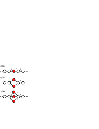
Figure 1: (Color online) Systems of parallel quantum dots. The tight-binding hopping parameter $t$ determines the half-width of the conduction band, $D=2t$, while parameter $t^{\prime}$ is related to the hybridization $\Gamma$ by $\Gamma/D=(t^{\prime}/t)^{2}$.

III Low-temperature effective models

Our primary goal is to demonstrate that the low-temperature effective model for the multiple impurity system is the $S=N/2$ $SU(2)$ Kondo model:

$$H=H_{\mathrm{band}}+\sum_{k^{\prime}k}J_{k^{\prime}k}\boldsymbol{s}_{kk^{\prime}}\cdot\boldsymbol{S},$$ (4)

where $\boldsymbol{s}_{kk^{\prime}}=\frac{1}{2}\sum_{\alpha\alpha^{\prime}}c^{\dagger}_{k\alpha}\boldsymbol{\sigma}_{\alpha\alpha^{\prime}}c_{k^{\prime}\alpha^{\prime}}$ is the local-spin density in the Wannier orbital in the conduction band that couples to all $N$ impurities. $\boldsymbol{S}$ is the collective impurity $S=N/2$ spin operator and $J_{k^{\prime}k}$ is the momentum-dependent anti-ferromagnetic spin-exchange interaction that can be derived using the Schrieffer-Wolff transformation. Results for $J_{k^{\prime}k}$ are independent of $N$.

We first argue in favor of the validity of the effective Hamiltonian, proposed in Eq. (4), by considering the different time scales of the original $N$-impurity Anderson problem. To simplify the argument we further focus on the (nearly) symmetric case $\delta\ll U$ within the Kondo regime, $U/(\Gamma\pi)\gg 1$.

The shortest time scale, $\tau_{U}\sim\hbar/U$, represents charge excitations. The longest time scale is associated with the Kondo effect (magnetic excitations) and it is given by $\tau_{K}\sim\hbar/T_{K}$ where $T_{K}$ is the Kondo temperature of the single impurity Anderson model, given by Haldane’s expression

$$T_{K}=0.182U\sqrt{\rho_{0}J_{\mathrm{K}}}\exp\left(-\frac{1}{\rho_{0}J_{\mathrm{K}}}\right),$$ (5)

where $J_{K}$ is the effective anti-ferromagnetic Kondo exchange interaction and $\rho_{0}J_{K}=8\Gamma/\pi U$. This expression is valid for $U\ll D$ and $\delta=0$.

As we will show later, there is an additional time scale $\tau_{J}\sim\hbar/J_{\mathrm{RKKY}}$, originating from the ferromagnetic RKKY dot-dot interactions:

$$J_{\mathrm{RKKY}}\sim U(\rho_{0}J_{K})^{2}=\frac{64}{\pi^{2}}\frac{\Gamma^{2}}{U}.$$ (6)

From the condition for a well developed Kondo effect, $U/(\Gamma\pi)\gg 1$, we obtain $J_{\mathrm{RKKY}}\ll U$. We thus establish a hierarchy of time scales $\tau_{U}\ll\tau_{J}\ll\tau_{K}$.

Based on the three different time-scales, we predict the existence of three distinct regimes close to the particle-hole symmetric point. The local moment regime is established at $T\sim T_{1}^{*}$, where $T_{1}^{*}=U/\alpha$ and $\alpha$ is a constant of the order one Krishnamurthy et al. (1980). In this regime the system behaves as $N$ independent spin $S=1/2$ impurities. At $T\sim T_{F}^{*}$, where $T_{F}^{*}=J_{\mathrm{RKKY}}/\beta$ and $\beta$ is a constant of the order one, spins bind into a high-spin $S=N/2$ state. With further lowering of the temperature, at $T\sim T_{K}$ the $S=N/2$ object experiences the Kondo effect which screens half a unit of spin (since there is a single conduction channel) to give a ground-state spin of $S-1/2=(N-1)/2$.

III.1 Schrieffer-Wolff transformation for multiple impurities

For $T<T_{1}^{*}$, the single impurity Anderson model can be mapped using the Schrieffer-Wolff transformation Schrieffer and Wolff (1966) to an $s-d$ exchange model (the Kondo model) with an energy dependent anti-ferromagnetic exchange interaction $J_{k^{\prime}k}$. In this subsection we show that for multiple impurities a generalized Schrieffer-Wolff transformation can be performed and that below $T_{1}^{*}$, the $N$-impurity Anderson model maps to the $N$-impurity $S=1/2$ Kondo model. Furthermore, the exchange constant is shown to be the same as in the single impurity case.

Due to the hybridization term $V_{k}$, the electrons are hopping on and off the impurities. Since all impurities are coupled to the same Wannier orbital, it could be expected that these hopping transitions would somehow “interfere”. It should be recalled, however, that the dwelling time $\tau_{U}$ is much shorter than the magnetic time scales $\tau_{J}$ and $\tau_{K}$. In other words, spin-flips are realized on a much shorter time-scale compared to the mean-time between successive spin-flips; for this reason, each local moment may be considered as independent. Note that the impurities do in fact “interfere”: there are ${\mathcal{O}}(V_{k}^{4})$ processes which lead to an effective ferromagnetic RKKY exchange interaction between pairs of spins and ultimately to the ferromagnetic ordering of spins at temperatures below $\sim J_{\mathrm{RKKY}}$. This will be discussed in the following subsection.

The Schrieffer-Wolff transformation is a canonical transformation that eliminates hybridization terms $V_{k}$ to first order from the Hamiltonian $H$, i.e. it requires that Schrieffer and Wolff (1966)

$${\bar{H}}\equiv e^{\mathcal{S}}He^{-{\mathcal{S}}}$$ (7)

have no terms which are first order in $V_{k}$. We expand ${\bar{H}}$ in terms of nested commutators:

$${\bar{H}}=H+[{\mathcal{S}},H]+\frac{1}{2}[{\mathcal{S}},[{\mathcal{S}},H]]+\ldots$$ (8)

and write $H=H_{0}+H_{c}$, where $H_{0}=H_{\mathrm{band}}+H_{\mathrm{dots}}$. We then choose ${\mathcal{S}}$ to be first order in $V_{k}$ so that

$$[{\mathcal{S}},H_{0}]+H_{c}=0.$$ (9)

As previously discussed, each impurity can be considered independent due to the separation of time scales. Therefore, we choose the generator ${\mathcal{S}}$ to be the sum ${\mathcal{S}}=\sum_{i}{\mathcal{S}}_{i}$ of generators ${\mathcal{S}}_{i}$, where the generator ${\mathcal{S}}_{i}$ for each impurity has the same form as in the single-impurity case:

$${\mathcal{S}}_{i}=\sum_{k\sigma\alpha}\frac{V_{k}}{\epsilon_{k}-\epsilon_{\alpha}}n_{i,-\sigma}^{\alpha}c_{k\sigma}^{\dagger}d_{i\sigma}-\text{H.c.}$$ (10)

with $\epsilon_{\pm}=\delta\pm U/2$ and the projection operators $n_{i,-\sigma}^{\alpha}$ are defined by

$$\begin{split}n_{i,-\sigma}^{+}&=n_{i,-\sigma},\\ n_{i,-\sigma}^{-}&=1-n_{i,-\sigma}.\end{split}$$ (11)

The resulting effective Hamiltonian is then given by

$$H_{\mathrm{eff}}=H_{0}+\frac{1}{2}[{\mathcal{S}},H_{c}],$$ (12)

which features $\mathcal{O}(V_{k}^{2})$ effective interactions with the leading terms that can be cast in the form of the Kondo antiferromagnetic exchange interaction

$$H_{\mathrm{ex}}=\sum_{i}\left(\sum_{kk^{\prime}}J_{k^{\prime}k}\boldsymbol{s}_{kk^{\prime}}\cdot\boldsymbol{S}_{i}\right),$$ (13)

where $\boldsymbol{S}_{i}$ is the $S=1/2$ spin operator on impurity $i$ defined by $\boldsymbol{S}_{i}=\frac{1}{2}\sum_{\alpha\alpha^{\prime}}d^{\dagger}_{i\alpha}\boldsymbol{\sigma}d_{i\alpha^{\prime}}$ and the exchange constant $J_{k^{\prime}k}$ is given by

$$\begin{split}J_{k^{\prime}k}=&V_{k^{\prime}}V_{k}\Bigl{(}\frac{1}{\epsilon_{k}-(\delta+U/2)}+\frac{1}{\epsilon_{k^{\prime}}-(\delta+U/2)}\\ &-\frac{1}{\epsilon_{k}-(\delta-U/2)}-\frac{1}{\epsilon_{k^{\prime}}-(\delta-U/2)}\Bigr{)}.\end{split}$$ (14)

If we limit the wave-vectors to the Fermi surface, i.e. for $k=k^{\prime}=k_{F}$, we obtain

$$J_{K}\equiv 2|V_{k_{F}}|^{2}\left(\frac{1}{|\delta-U/2|}+\frac{1}{|\delta+U/2|}\right).$$ (15)

This result is identical to $J_{k^{\prime}k}$ obtained for a single impurity Schrieffer and Wolff (1966).

As it turns out, the Schrieffer-Wolff transformation, Eqs. (7)-(12), produces inter-impurity interaction terms in addition to the expected impurity-band interaction terms. In the particle-hole symmetric case ($\delta=0$), these additional terms can be written as

$$\Delta H_{\mathrm{eff}}=2\frac{|V_{k}|^{2}}{U}\left(\sum_{i=1}^{N}n_{i}-N\right)h_{\mathrm{hop}},$$ (16)

where

$$h_{\mathrm{hop}}=\sum_{i<j,\sigma}\left(d^{\dagger}_{i\sigma}d_{j\sigma}+d^{\dagger}_{j\sigma}d_{i\sigma}\right).$$ (17)

Since the on-site charge repulsion favors states with single occupancy of each impurity, the term in the parenthesis in Eq. (16) is on the average equal to zero. Furthermore, if each site is singly occupied, possessing small fluctuations of the charge $\langle n_{i}^{2}\rangle-\langle n_{i}\rangle^{2}\sim 0$, hopping between the sites is suppressed and the term $h_{\mathrm{hop}}$ represents another small factor. The Hamiltonian $\Delta H$ is thus clearly not relevant: impurities are indeed independent.

On departure from the particle-hole symmetric point ($\delta\neq 0$), $\Delta H_{\mathrm{eff}}$ generalizes to

$$\Delta H_{\mathrm{eff}}=2\frac{U|V_{k}|^{2}}{U^{2}-4\delta^{2}}\left(\left(\sum_{i=1}^{2}n_{i}-N\right)-2N\frac{\delta}{U}\right)h_{\mathrm{hop}}.$$ (18)

For moderately large $\delta/U$ this Hamiltonian term still represents only a small correction to Eq. (13). However, for strong departure from the particle-hole (p-h) symmetric point, close to the valence-fluctuation regime (i.e. $\delta\to U/2$), the $\Delta H_{\mathrm{eff}}$ becomes comparable in magnitude to $H_{\mathrm{ex}}$ and generates hopping of electrons between the impurities.

The above discussion leads us to the conclusion that just below $T_{1}^{*}$ the effective Hamiltonian close to the p-h symmetric point is

$$H_{\mathrm{eff}}=H_{\mathrm{band}}+\sum_{i}\sum_{k^{\prime}k}J_{k^{\prime}k}\boldsymbol{s}_{kk^{\prime}}\cdot\boldsymbol{S}_{i}.$$ (19)

If the dots are described by unequal Hamiltonians $H_{\mathrm{dot},i}$ or have unequal hybridizations $V^{i}_{k}$, then the mapping of the multi-impurity Anderson model to a multi-impurity Kondo model still holds, however with different effective exchange constants $J_{k^{\prime}k}^{i}$.

III.2 RKKY interaction and ferromagnetic spin ordering

We now show that the effective RKKY exchange interaction between the spins in the effective $N$-impurity Kondo model, Eq. (19), is ferromagnetic and also responsible for locking of spins in a state of high total spin for temperatures below $T<J_{\rm RKKY}$.

The ferromagnetic character of the RKKY interaction is expected, as shown by the following qualitative argument. We factor out the spin operators in the effective Hamiltonian Eq. (19):

$$H_{\mathrm{eff}}=H_{\mathrm{band}}+\left(\sum_{k^{\prime}k}J_{k^{\prime}k}\boldsymbol{s}_{kk^{\prime}}\right)\cdot\sum_{i}\boldsymbol{S}_{i}.$$ (20)

Spins $\boldsymbol{S}_{i}$ are aligned in the ground state since such orientation minimizes the energy of the system. This follows from considering a spin chain with $N$ sites in a “static magnetic field” $\sum_{k^{\prime}k}J_{k^{\prime}k}\boldsymbol{s}_{kk^{\prime}}$. The assumption of a static magnetic field is valid due to the separation of relevant time scales, $\tau_{K}\gg\tau_{J}$. States with $S<N/2$ are clearly excited states with one or several “misaligned” spins.

Since the inter-dot spin-spin coupling is a special case of the Ruderman-Kittel-Kasuya-Yosida (RKKY) interaction in bulk systems Ruderman and Kittel (1954), a characteristic functional dependence given by

$$J_{\mathrm{RKKY}}\propto U(\rho_{0}J_{\mathrm{K}})^{2}=\frac{64}{\pi^{2}}\frac{\Gamma^{2}}{U}=\frac{16V_{k_{F}}^{4}}{U},$$ (21)

is expected. The factor $U$ in front of $(\rho_{0}J_{K})^{2}$ plays the role of a high-energy cut-off, much like the $0.196U$ effective-bandwidth factor in the expression for $T_{K}$, Eq. (5).

Using the Rayleigh-Schrödinger perturbation theory we calculated the singlet and triplet ground state energies $E_{S}$ and $E_{T}$ to the fourth order in $V_{k}$ for the two-impurity case (see Appendix A). We define the RKKY exchange parameter by $J_{\mathrm{RKKY}}=E_{S}-E_{T}$; positive value of $J_{\mathrm{RKKY}}$ corresponds to ferromagnetic RKKY interaction. For $U/d\lesssim 0.1$, the prefactor of $(\rho_{0}J_{K})^{2}$ in the expression (21) is indeed found to be linear in $U$. Together with the prefactor the perturbation theory leads to

$$J_{\mathrm{RKKY}}=0.62U(\rho_{0}J_{K})^{2}\quad\text{for}\quad U/D\ll 1,$$ (22)

which, as we will show later, fits very well our numerical results. The RKKY interaction becomes fully established for temperatures below $T_{J}$ which is roughly one or two orders of magnitude smaller than $T_{1}^{*}$ ($T_{J}$ is defined in Appendix A). Since the RKKY interactions in the first approximation do not depend much on the number of impurities, for $N>2$ the exchange interaction between each pair of impurities has the same strength as in the two impurity case. Therefore, for temperatures just below $T_{J}$, the effective Hamiltonian for the $N$-impurity Anderson model becomes

$$H_{\mathrm{eff}}=H_{\mathrm{band}}+\left(\sum_{k^{\prime}k}J_{k^{\prime}k}\boldsymbol{s}_{kk^{\prime}}\right)\cdot\sum_{i}\boldsymbol{S}_{i}-J_{\mathrm{RKKY}}\sum_{i<j}\boldsymbol{S}_{i}\cdot\boldsymbol{S}_{j}.$$ (23)

When the temperature drops below a certain temperature $T_{F}^{*}$, the spins align and form a ferromagnetically-frozen state of maximum spin $S=N/2$. The transition temperature $T_{F}^{*}$ is generally of the same order as $J_{\mathrm{RKKY}}$, i.e. $T_{F}^{*}=J_{\mathrm{RKKY}}/\beta$, where $\beta$ is an $N$-dependent constant of the order one. This relation holds if $T_{F}^{*}\ll T_{J}$, otherwise $T_{F}^{*}$ needs to be determined using a self-consistency equation (57), as discussed in Appendix A.

In conclusion, for $T\lesssim T_{F}^{*}$ the states with total spin less than $N/2$ can be neglected, and the system behaves as if it consisted of a single spin $\boldsymbol{S}$ of magnitude $S=N/2$. The effective Hamiltonian at very low temperatures is therefore the $S=N/2$ $SU(2)$ Kondo model

$$H_{\mathrm{eff}}=H_{\mathrm{band}}+\sum_{k,k^{\prime}}J_{k^{\prime}k}\boldsymbol{s}_{k,k^{\prime}}\cdot\boldsymbol{S},$$ (24)

where $\boldsymbol{S}={\mathcal{P}}\left(\sum_{i}\boldsymbol{S}_{i}\right){\mathcal{P}}$ and ${\mathcal{P}}$ is the projection operator on the subspace with total spin $S=N/2$. Other multiplets are irrelevant at temperatures below $T_{F}^{*}$. We point out that the Kondo temperature for this model is given by the formula for the single impurity Anderson model, Eq. (5), irrespective of the number of dots $N$, since the ferromagnetic interaction only leads to moment ordering, while the exchange interaction of the collective spin is still given by the same $J_{k^{\prime}k}$.

It should be mentioned that if the exchange constants $J^{i}_{k^{\prime}k}$ for different impurities are different, there will be some mixing between the spin multiplets. The simple description of impurities as a collective $S=N/2$ spin still holds even for relatively large differences, but in general the virtual excitations to other spin multiplets must be taken into account. This is studied in detail for the case of two dots in Section VI.4.

IV The methods

IV.1 Numerical renormalization group

The method of choice to study the low-temperature properties of quantum impurity models is the Wilson’s numerical renormalization group (NRG) Wilson (1975); Krishnamurthy et al. (1980); Krishnaurthy et al. (1980). The NRG technique consists of logarithmic discretization of the conduction band described by $H_{\mathrm{band}}$, mapping onto a one-dimensional chain with exponentially decreasing hopping constants, and iterative diagonalization of the resulting Hamiltonian. Since all $N$ impurities couple to the band in the same manner, they all couple to the same, zero-th site of the chain Hamiltonian Krishnamurthy et al. (1980):

$$\begin{split}\frac{H_{C}}{D}&=\frac{1}{2}(1+\Lambda^{-1})\\ &\sum_{n=0}^{\infty}\sum_{\sigma}\Lambda^{-n/2}\xi_{n}\left[f^{\dagger}_{n,\sigma}f_{n+1,\sigma}+f^{\dagger}_{n+1,\sigma}f_{n,\sigma}\right]\\ &+H_{\mathrm{dots}}+\sum_{i,\sigma}\left(\frac{2\Gamma}{\pi D}\right)^{1/2}\left(f^{\dagger}_{0\sigma}d_{i\sigma}+d^{\dagger}_{i\sigma}f_{0\sigma}\right).\end{split}$$ (25)

Here $f^{\dagger}_{n\sigma}$ are the chain creation operators and $\xi_{n}$ are constants of order 1. In addition to the conventional Wilson’s discretization scheme Wilson (1975), we also used Campo and Oliveira’s new discretization approach using an over-complete basis of states Campo and Oliveira (2005) with $\Lambda=4$, which improved convergence to the continuum limit. We made use of the “$z$-trick” with typically 6 equally spaced values of the parameter $z$ Oliveira and Oliveira (1994).

IV.1.1 Symmetries

The Hamiltonian (1) has the following symmetries: a) $U(1)_{\mathrm{gauge}}$ symmetry due to global phase (gauge) invariance. The corresponding conserved quantity is the total charge (defined with respect to half-filling case): $Q=\sum_{i}\left(n_{i}-1\right)$, where the sum runs over all the impurity as well as the lead sites; b) $SU(2)_{\mathrm{spin}}$ spin symmetry with generators $\boldsymbol{S}=\sum_{i}\frac{1}{2}\sum_{\alpha\alpha^{\prime}}a^{\dagger}_{i\alpha}\boldsymbol{\sigma}_{\alpha\alpha^{\prime}}a_{i\alpha^{\prime}}$, where $\boldsymbol{\sigma}$ are the Pauli matrices. Since operators $Q$, $\boldsymbol{S}^{2}$ and $S_{z}$ commute with $H$, the invariant subspaces can be classified according to quantum numbers $Q$, $S$ and $S_{z}$. Computation of matrix elements can be further simplified using the Wigner-Eckart theorem Krishnamurthy et al. (1980).

In the particle-hole symmetric point, i.e. $\delta=0$, Hamiltonian has an additional $SU(2)_{\mathrm{iso}}$ isospin symmetry Jones et al. (1988). We define isospin operators on impurity site $i$ using

$$\boldsymbol{I}_{i}=\sum_{\alpha\alpha^{\prime}}\eta^{\dagger}_{i,\alpha}\boldsymbol{\sigma}_{\alpha\alpha^{\prime}}\eta_{i,\alpha^{\prime}},$$ (26)

where the Nambu spinor $\eta^{\dagger}_{i}$ on the impurity orbitals is defined by

$$\eta^{\dagger}_{i}=\begin{pmatrix}d^{\dagger}_{i,\uparrow}\\ -d_{i,\downarrow}\end{pmatrix}.$$ (27)

We also define $I^{+}=I^{x}+iI^{y}$ and $I^{-}=(I^{+})^{\dagger}$. We then have, for example, $I^{z}_{i}=(n_{i}-1)/2=Q_{i}/2$ and $I^{+}_{i}=d^{\dagger}_{i\downarrow}d^{\dagger}_{i\uparrow}$. The isospin symmetry is thus related to the electron pairing. In terms of the isospin operators the impurity Hamiltonian can be written as

$$H_{\mathrm{dot},i}=2\delta I^{z}_{i}+4U(I^{z}_{i})^{2}=2\delta I^{z}_{i}+\frac{4}{3}U(I_{i})^{2},$$ (28)

where we took into account that for spin-1/2 operators (Pauli matrices) $(I_{i}^{z})^{2}=1/3(I_{i})^{2}$.

On the Wilson chain the isospin is defined similarly but with a sign alternation in the definition of the Nambu spinors $\xi_{n}$:

$$\xi^{\dagger}_{n}=\begin{pmatrix}f^{\dagger}_{n,\uparrow}\\ (-1)^{n}f_{n,\downarrow}\end{pmatrix}.$$ (29)

The total isospin operator is obtained through a sum of $\boldsymbol{I}_{i}$ for all orbitals of the problem (impurities and conduction band). For $\delta=0$, both $\boldsymbol{I}^{2}$ and $I_{z}$ commute with $H$ and $I$ and $I_{z}$ are additional good quantum numbers. Note that $I_{z}=Q/2$, therefore $U(1)_{\mathrm{gauge}}$ is in fact a subgroup of $SU(2)_{\mathrm{iso}}$. Due to isotropy in isospin space, the $I_{z}$ dependence can again be taken into account using the Wignert-Eckart theorem.

Spin and isospin operators commute, $[S_{i},I_{j}]=0$ for all $i,j$. Therefore, for $\delta=0$ the problem has a $SU(2)_{\mathrm{spin}}\otimes SU(2)_{\mathrm{iso}}$ symmetry which, when explicitly taken into account, leads to a further significant reduction of the numerical task.

In all our NRG calculations we took into account the conservation of the charge and the rotational invariance in the spin space, i.e. the $U(1)_{\mathrm{gauge}}\otimes SU(2)_{\mathrm{spin}}$ symmetry which holds for all perturbed models considered, or the $SU(2)_{\mathrm{spin}}\otimes SU(2)_{\mathrm{isospin}}$ symmetry where applicable. The number of states that we kept in each stage of the NRG iteration depended on the number of the dots $N$, since the degeneracy increases exponentially with $N$: approximately as $4^{N}$ at the high-temperature free orbital regime and as $2^{N}$ in the local-moment regime. In the most demanding $N=4$ calculation we kept up to 12000 states at each iteration (which corresponds to $>32000$ states taking into account the spin multiplicity of states), which gave fully converged results for the magnetic susceptibility.

For large scale NRG calculations it is worth taking into account that the calculation of eigenvalues scales as ${\mathcal{O}}(n^{2})$ and the calculation of eigenvectors as ${\mathcal{O}}(n^{3})$, where $n$ is the dimension of the matrix being diagonalized. Since eigenvectors of the states that are truncated are not required to recalculate various matrices prior to performing a new iteration, considerable amount of time can be saved by not calculating them at all.

IV.1.2 Calculated quantities

We have computed the following thermodynamic quantities

• the temperature-dependent impurity contribution to the magnetic susceptibility $\chi_{\mathrm{imp}}(T)$

  $$\chi_{\mathrm{imp}}(T)=\frac{(g\mu_{B})^{2}}{k_{B}T}\left(\langle S_{z}^{2}\rangle-\langle S_{z}^{2}\rangle_{0}\right)$$ (30)

  where the subscript $0$ refers to the situation when no impurities are present (i.e. $H$ is simply the band Hamiltonian $H_{\mathrm{band}}$), $g$ is the electronic $g$ factor, $\mu_{B}$ the Bohr magneton and $k_{B}$ the Boltzmann’s constant. It should be noted that the combination $T\chi_{\mathrm{imp}}/(g\mu_{B})^{2}$ can be considered as an effective moment of the impurities, $\mu_{\mathrm{eff}}$.

• the temperature-dependent impurity contribution to the entropy $S_{\mathrm{imp}}(T)$

  $$S_{\mathrm{imp}}(T)=\frac{\left(E-F\right)}{T}-\frac{\left(E-F\right)_{0}}{T},$$ (31)

  where $E=\langle H\rangle=\mathrm{Tr}\left(He^{-H/(k_{B}T)}\right)$ and $F=-k_{B}T\ln\mathrm{Tr}\left(e^{-H/k_{B}T}\right)$. From the quantity $S_{\mathrm{imp}}/k_{B}$ we can deduce the effective degrees-of-freedom $\nu$ of the impurity as $S_{\mathrm{imp}}/k_{B}\sim\ln\nu$.

• thermodynamic expectation values of various operators such as the on-site occupancy $\langle n_{i}\rangle$, local charge-fluctuations $\langle(\delta n)^{2}\rangle=\langle n_{i}^{2}\rangle-\langle n_{i}\rangle^{2}$, local-spin $\langle\boldsymbol{S}_{i}^{2}\rangle$ and spin-spin correlations $\langle\boldsymbol{S}_{i}\cdot\boldsymbol{S}_{j}\rangle$.

In the following we drop the suffix $\mathrm{imp}$ in $\chi_{\mathrm{imp}}$, but one should keep in mind that impurity contribution to the quantity is always implied. We also set $k_{B}=1$.

IV.2 Bethe Ansatz

The single-channel $SU(2)$ Kondo model can be exactly solved for an arbitrary spin of the impurity using the Bethe Ansatz (BA) method Andrei et al. (1983); Rajan et al. (1982); Sacramento and Schlottmann (1989). This technique gives exact results for thermodynamic quantities, such as magnetic susceptibility, entropy and heat capacity. It is, however, incapable of providing spectral and transport properties. For the purpose of comparing results of the single-channel $SU(2)$ Kondo model with NRG results of the N-impurity Anderson model, we have numerically solved the system of coupled integral equations using a discretization scheme as described, for example, in Ref. Sacramento and Schlottmann, 1989.

IV.3 Scaling analysis

Certain aspects of the Kondo physics can be correctly captured using the perturbative renormalization group approach based on the “poor-man’s scaling” technique due to Anderson Anderson (1970). A brief account of this method is given in Appendix B.

V Numerical results

We choose the parameters $U$ and $\Gamma$ so that the relevant energy scales are well separated which enables clear identification of various regimes and facilitates analytical predictions.

In Fig. 2 we show temperature dependence of magnetic susceptibility and entropy for $N=1,2,3$ and 4 systems. As the temperature is reduced, the system goes through the following regimes:

1. At high temperatures, $T>T_{1}^{*}$, the impurities are independent and they are in the free orbital regime (FO) (states $|0\rangle$, $|\uparrow\rangle$, $|\downarrow\rangle$ and $|2\rangle$ on each impurity are equiprobable). Each dot then contributes $1/8$ to $\mu_{\mathrm{eff}}=T\chi/(g\mu_{B})^{2}$ for a total of $\mu_{\mathrm{eff}}=N/8$. The entropy approaches $S_{\mathrm{imp}}=N\ln 4$ since all possible states are equally probable Krishnamurthy et al. (1980).

2. For $T_{F}^{*}<T<T_{1}^{*}$ each dot is in the local-moment regime (LM) (states $|\uparrow\rangle$ and $|\downarrow\rangle$ are equiprobable, while the states $|0\rangle$ and $|2\rangle$ are suppressed). Each dot then contributes $1/4$ to $\mu_{\mathrm{eff}}$ for a total of $N/4$. The entropy decreases to $S_{\mathrm{imp}}=N\ln 2$.

3. For $T_{K}<T<T_{F}^{*}$ and $N\geq 1$ the dots lock into a high spin state $S=N/2$ due to ferromagnetic RKKY coupling between local moments formed on the impurities. This is the ferromagnetically frozen regime (FF) Jayaprakash et al. (1981) with $\mu_{\mathrm{eff}}=S(S+1)/3=N/2(N/2+1)/3$. The entropy decreases further to $S_{\mathrm{imp}}=\ln(2S+1)=\ln(N+1)$.

4. Finally, for $T<T_{K}$, the total spin is screened from $S=N/2$ to $\tilde{S}=S-1/2=(N-1)/2$ as we enter the partially-quenched, Kondo screened strong-coupling (SC) $N$-impurity regime with $\mu_{\mathrm{eff}}=\tilde{S}(\tilde{S}+1)/3=(N-1)/2[(N-1)/2+1]/3$. The remaining $S-1/2$ spin is a complicated object: a $S=N/2$ multiplet combination of the impurity spins antiferromagnetically coupled by a spin-$1/2$ cloud of the lead Jayaprakash et al. (1981). In this regime, the entropy reaches its minimum value of $S_{\mathrm{imp}}=\ln(2{\tilde{S}}+1)=\ln N$.

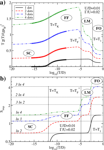
Figure 2: (Color online) a) Temperature-dependent susceptibility and b) entropy of the $N$-dot systems calculated using the NRG. The symbols in the susceptibility plots were calculated using the thermodynamic Bethe Ansatz approach for the corresponding $S=N/2$ SU(2) Kondo models ($\bullet$ $S=1/2$, $\blacksquare$ $S=1$, $\blacklozenge$ $S=3/2$, $\blacktriangle$ $S=2$).

$N$	Kondo temperature $T_{K}/D$	LM-FO temperature $T_{F}^{*}/D$
1	$1.20\times 10^{-12}$	-
2	$1.23\times 10^{-12}$	$1.87\times 10^{-5}$
3	$1.29\times 10^{-12}$	$2.11\times 10^{-5}$
4	$1.32\times 10^{-12}$	$2.32\times 10^{-5}$

Table 1: Kondo temperatures for different numbers of quantum dots $N$ corresponding to plots in Fig. 2.

In Fig. 2, atop the NRG results we additionally plot the results for the magnetic susceptibility of the $S=N/2$ $SU(2)$ Kondo model obtained using an exact thermodynamic Bethe-Ansatz method. For $T<T_{F}^{*}$ nearly perfect agreement between the $N$-impurity Anderson model and the corresponding $S=N/2$ $SU(2)$ Kondo model are found over many orders of magnitude. This agreement is used to extract the Kondo temperature of the multiple-impurity Anderson model. The fitting is performed numerically by the method of least-squares; in this manner very high accuracy of the extracted Kondo temperature can be achieved. The results in Table 1 point out the important result of this work that the Kondo temperature is nearly independent of $N$, as predicted in Section III.2. In this sense, the locking of spins into a high-spin state does not, by itself, weaken the Kondo effect Craig et al. (2004); Vavilov and Glazman (2005); however, it does modify the temperature-dependence of the thermodynamic and transport properties Mehta et al. (2005); Koller et al. (2005).

It is instructive to follow transitions from high-temperature FO regime to LM and FF regime through a plot combining the temperature dependence of the magnetic susceptibility and of other thermodynamic quantities, as presented in Fig. 3. Charge fluctuations $\langle(\delta n)^{2}\rangle$ show a sudden drop at $T\sim T_{1}^{*}$ representing the FO - LM transition. In contrast, the magnitude of the total spin $S$ increases in steps: $S=1/2$, $(\sqrt{7}-1)/2$ and $1$. Values of $S$ in these plateaus are the characteristic values of doubly occupied double-quantum dot system in the FO, LM and FF regime, respectively.

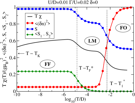
Figure 3: (Color online) Temperature-dependence of susceptibility, charge fluctuations $\langle(\delta n)^{2}\rangle$, total spin $S$ and the spin-spin correlations $\langle\boldsymbol{S}_{1}\cdot\boldsymbol{S}_{2}\rangle$ of the 2-dot system.

The LM-FF transition temperature $T_{F}^{*}$ can be deduced from the temperature dependence of the spin-spin correlation function. In the FF regime the spins tend to align, which leads to $\langle{\bf S}_{1}\cdot{\bf S}_{2}\rangle\to\sim 1/4$ as $T\to 0$, see Fig. 3. The transition from 0 to $1/4$ is realized at $T\sim T_{F}^{*}$. We can extract $T_{F}^{*}$ using the (somewhat arbitrary) condition

$$\langle{\bf S}_{1}\cdot{\bf S}_{2}\rangle(T_{F}^{*})=1/2\langle{\bf S}_{1}\cdot{\bf S}_{2}\rangle(T\to 0).$$ (32)

In section VI.2.1 we show that this condition is in very good agreement with $T_{F}^{*}=J_{\mathrm{RKKY}}/\beta$ obtained by determining the explicit inter-impurity antiferromagnetic coupling constant $J_{12}$, defined by the relation $J_{\mathrm{RKKY}}+J_{12}=0$ that destabilizes the high-spin $S=N/2$ state. The extracted $T_{F}^{*}$ transition temperatures that correspond to plots in Fig. 2 are given in Table 1. We find that they weakly depend on the number of impurities, more so than the Kondo temperature. The increase of $T_{F}^{*}$ with $N$ can be partially explained by calculating $T_{F}^{*}$ for a spin Hamiltonian $H=-J_{\mathrm{RKKY}}\sum_{i<j}\boldsymbol{S}_{i}\cdot\boldsymbol{S}_{j}$ for $N$ spins decoupled from leads. Using Eq. (32) we obtain $T_{F}^{*}\approx 1.18\ J_{\mathrm{RKKY}}$ for $N=2$, $T_{F}^{*}\approx 1.36\ J_{\mathrm{RKKY}}$ for $N=3$ and $T_{F}^{*}\approx 1.55\ J_{\mathrm{RKKY}}$ for $N=4$.

By performing NRG calculations of $T_{F}^{*}$ for other parameters $U$ and $\Gamma$ and comparing them to the prediction of the perturbation theory, we found that the simple formula (22) for $J_{\mathrm{RKKY}}$ agrees very well with numerical results.

The effect on thermodynamic properties of varying $U$ while keeping $\Gamma/U$ (i.e. $\rho_{0}J_{\mathrm{K}}$) fixed is illustrated in Fig. 4 for 2- and 3-dot systems. Parameters $\Gamma$ and $U$ enter expressions for $T_{F}^{*}=J_{\mathrm{RKKY}}/\beta$ and $T_{K}$ only through the ratio $\Gamma/U$, apart from the change of the effective bandwidth proportional to $U$, see Eq. (5) and (22). This explains the horizontal shift towards higher temperatures of susceptibility curves with increasing $U$, as seen in Fig. 4a. The NRG results and the Bethe-Ansatz for the Kondo models with $S=1$ and $S=3/2$ show excellent agreement for $T<T_{F}^{*}$. In Figs. 4b and 4c we demonstrate the nearly linear $U$-dependence of $T_{F}^{*}$ and $T_{K}$, respectively.

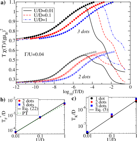
Figure 4: (Color online) a) Temperature-dependent susceptibility of the 2 and 3-dot systems with the same $\Gamma/U$ ratio. Open (filled) symbols are Bethe-Ansatz results for the $S=1$ ($S=3/2$) Kondo model. b) Comparison of LM-FF transition temperature $T_{F}^{*}$ with predictions of the perturbation theory. c) Comparison of calculated $T_{K}$ with the Haldane’s formula.

In Fig. 5 we show the effect of varying $\Gamma/U$ while keeping $U$ fixed. In this case, $T_{1}^{*}$ stays the same, $T_{F}^{*}$ is shifted quadratically and $T_{K}$ exponentially with increasing $\Gamma/U$. Fig. 5b shows the agreement of $T_{F}^{*}$ with expression (22), while Fig. 5c shows the agreement of the extracted values of $T_{K}$ with formula (5).

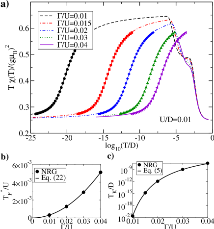
Figure 5: (Color online) a) Temperature-dependent susceptibility of the 2-dot system for equal e-e repulsion $U/D=0.01$ and for different hybridization strengths $\Gamma$. Symbols represent the Bethe-Ansatz susceptibility for the $S=1$ Kondo model with corresponding $T_{K}$. b) Comparison of calculated and predicted $T_{F}^{*}$. c) Fit of $T_{K}$ to the Haldane’s formula, Eq. (5).

We note that for $N\geq 2$, eventual coupling to an additional conduction channel (for example, due to a small asymmetry in the coupling to the source and drain electrodes) would lead to screening by additional half a unit of spin Jayaprakash et al. (1981); Silva et al. (1996) and the residual ground state spin would be $S-1=N/2-1$. For $N\geq 3$ and three channels (due to weak coupling to some third electrode), three half-units of spin would be screened, and so forth. These additional stages of Kondo screening would, however, occur at much lower temperatures; all our findings still apply at temperatures above subsequent Kondo cross-overs.

In systems of multiple quantum dots, an additional screening mechanism is possible when after the first Kondo cross-over, the residual interaction between the remaining spin and the Fermi liquid quasi-particles is antiferromagnetic Vojta et al. (2002). This leads to an additional Kondo cross-over at temperatures that are exponentially smaller than the first Kondo temperature. Such two-stage Kondo effect occurs, for example, in side-coupled double quantum dots Vojta et al. (2002); Cornaglia et al. (2004); Žitko and Bonča (2006); Hofstetter and Schoeller (2002) and triple quantum dot coupled in series Žitko et al. . In parallelly coupled systems, the residual interaction between the remaining spin and the Fermi liquid quasi-particles is, however, ferromagnetic as can be deduced from the splitting of the NRG energy levels in the strong-coupling fixed point Koller et al. (2005): the strong-coupling fixed point is stable.

We have thus demonstrated that with decreasing temperature the symmetric ($\delta=0$) multi-impurity Anderson model flows from the FO regime, through LM and FF regimes, to a stable underscreened $S=N/2$ Kondo model strong-coupling fixed point. The summary of different regimes is given in Table 2.

Regime	Relevant states	Magnetic susceptibility	Spin correlations	Charge fluctuations	Entropy
		$\mu_{\mathrm{eff}}=T\chi_{\mathrm{imp}}(T)/(g\mu_{B})^{2}$	$\langle\boldsymbol{S}_{1}\cdot\boldsymbol{S}_{2}\rangle$	$\langle n^{2}\rangle-\langle n\rangle^{2}$	$S_{\mathrm{imp}}$
FO	$N\times(|0\rangle,|\uparrow\rangle,|\downarrow\rangle,|2\rangle)$	$N/8$	$0$	$O(1)$	$N\ln 4$
LM	$N\times(|\uparrow\rangle,|\downarrow\rangle)$	$N/4$	$0$	small	$N\ln 2$
FF	$|S=N/2,S_{z}\rangle$	$N/2(N/2+1)/3$	$\sim 1/4$	small	$\ln(N+1)$
SC	$|S=N/2-1/2,S_{z}\rangle$	$(N-1)/2(N/2+1/2)/3$	$\sim 1/4$	small	$\ln N$

Table 2: Regimes of the symmetric ($\delta=0$) $N$-impurity Anderson model

VI Stability of $N=2$ systems with respect to various perturbations

We next explore the effect of various physically relevant perturbations with a special emphasis on the robustness of the ferromagnetically frozen state and the ensuing $S=N/2$ Kondo effect against perturbation of increasing strength. We show that the system of multiple quantum dots remains in a $S=N/2$ state even for relatively large perturbations. We also study the quantum phase transitions from the $S=N/2$ state driven by strong perturbations. In this sections we limit our calculations to the $N=2$ system.

VI.1 Variation of the on-site energy levels

VI.1.1 Deviation from the particle-hole symmetric point

A small departure from the particle-hole symmetric point ($\delta\neq 0$) does not destabilize the $S=N/2$ Kondo behavior: the magnetic susceptibility curves still follow the Bethe-Ansatz results even for $\delta/U$ as large as $0.4$, see Fig. 6a. For $\delta>\delta_{c}$, where $\delta_{c}/D\sim 0.45$ is the critical value of parameter $\delta$, the triplet state is destabilized. Consequently, there is no Kondo efect. This is a particular case of the singlet-triplet transition that is a subject of intense studies in recent years, both experimentally Entin-Wohlman et al. (2001); Fuhrer et al. (2004); Kogan et al. (2003) and theoretically Izumida et al. (2001); Pustilnik and Glazman (2001); Pustilnik et al. (2003); Hofstetter and Schoeller (2002); Hofstetter and Zarand (2004).

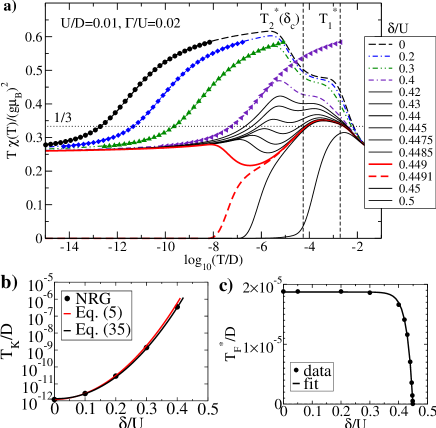
Figure 6: (Color online) a) Temperature-dependent susceptibility of the 2-dot systems on departure ($\delta>0$) from the particle-hole symmetric point, $\delta=0$. Symbols are fits to the universal susceptibility obtained using the Bethe-Ansatz method for the $S=1$ Kondo model. b) Calculated and predicted Kondo temperature, Eq. (35). For comparison we also plot $T_{K}$ given by Eq. (5), which shows expected discrepancy for large $\delta/U$. c) Calculated $T_{F}^{*}$ and the fit to an exponential function.

In the asymmetric single impurity model, the valence-fluctuation (VF) regime is characterized by $\mu_{\mathrm{eff}}=T\chi(T)/(g\mu_{B})^{2}\sim 1/6$ Krishnaurthy et al. (1980). The VF regimes occurs at $T_{1}^{*}$ and the transition from VF to LM regime occurs at $T_{2}^{*}\sim|E_{d}^{*}|/\alpha$, where $E_{d}^{*}$ is the renormalized on-site energy of the impurity: $E_{d}^{*}=\epsilon_{d}-\frac{\Gamma}{\pi}\ln\left(-U/E_{d}^{*}\right)$. For two uncorrelated dots in the VF regime, we expect $\mu_{\mathrm{eff}}\sim 1/3$. In Fig. 6a we plotted a number of susceptibility curves for parameters $\delta$ in the proximity of the singlet-triplet transition. While there is no clearly-observable valence-fluctuation plateau, the value of $\mu_{\mathrm{eff}}$ is indeed near $1/3$ between $T_{1}^{*}$ and $T_{2}^{*}(\delta_{c})$.

In Fig. 6b we compare calculated Kondo temperatures with analytical predictions based on the results for the single impurity model Krishnaurthy et al. (1980). For $\delta\neq 0$, $J_{\mathrm{K}}$ generalizes according to the Schrieffer-Wolff transformation, Eq. (15). Departure from the p-h symmetric point also induces potential scattering

$$\rho_{0}K=\frac{\Gamma}{2\pi}\left(\frac{1}{|\delta-U/2|}-\frac{1}{|\delta+U/2|}\right).$$ (33)

The effective ${\tilde{J}}_{\mathrm{K}}$ that enters the expression for the Kondo temperature is Krishnaurthy et al. (1980)

$${\tilde{J}}_{\mathrm{K}}=J_{\mathrm{K}}\left[1+\left(\pi\rho_{0}K\right)^{2}\right],$$ (34)

and the effective bandwidth $0.182U$ is replaced by $0.182|E_{d}^{*}|$. The Kondo temperature is now given by

$$T_{K}=0.182|E_{d}^{*}|\sqrt{\rho_{0}{\tilde{J}}_{\mathrm{K}}}\exp\left(-1/(\rho_{0}{\tilde{J}}_{\mathrm{K}})\right).$$ (35)

This analytical estimate agrees perfectly with the NRG results: for moderate $\delta/U$, the results obtained for asymmetric single impurity model also apply to the multi-impurity Anderson model.

In Fig. 6c we show the $\delta$-dependence of the LM-FF transition temperature $T_{F}^{*}$. Its value remains nearly independent of $\delta$ in the interval $\delta\lesssim 0.4U$ and then it suddenly drops. More quantitatively, the dependence on $\delta$ can be adequately described using an exponential function

$$T_{F}^{*}(\delta)=T_{F}^{*}(0)\left[1-\exp\left(\frac{\delta-\delta_{c}}{\lambda}\right)\right]$$ (36)

where $T_{F}^{*}(0)/D=1.8\times 10^{-5}$ is the transition temperature in the symmetric case, $\delta_{c}/D=0.45$ is the critical $\delta$ and $\lambda/D=2.1\times 10^{-2}$ is the width of the transition region. Exchange interaction $J_{\mathrm{RKKY}}$ does not depend on $\delta$ for $U/D=0.01\ll 1$, which explains constant value of $T_{F}^{*}(\delta)$ for $\delta\lesssim 0.4U$. At a critical value $\delta_{c}$, $T_{F}^{*}$ goes to zero and for still higher $\delta$ the spin-spin correlation becomes antiferromagnetic. Since the ground-state spins are different, the triplet and singlet regime are separated by a quantum phase transition at $\delta=\delta_{c}$. This transition is induced by charge fluctuations which destroy the ferromagnetic order of spins as the system enters the VF regime. The exponential dependence arises from the grand-canonical statistical weight factor $\exp[\delta(n-2)/(k_{B}T)]$, where $n$ is the number of the electrons confined on the dots. The transition is of the first order, since for equal coupling of both impurities to the band there is no mixing between the $n=2$ triplet states and the $n=0$ singlet state Vojta et al. (2002).

For $\delta$ slightly lower than the critical $\delta_{c}$, the effective moment $T\chi(T)$ shows a rather unusual temperature dependence. It first starts decreasing due to charge fluctuations, however with further lowering of the temperature the moment ordering wins over, $T\chi(T)$ increases and at low-temperatures approaches the value characteristic for the partially screened $S=1$ moment, i.e. $T\chi/(g\mu_{B})^{2}\sim 1/4$.

VI.1.2 Splitting of the on-site energy levels

We next consider the 2-dot Hamiltonian with unequal on-site energies $\delta_{i}$:

$$H_{\mathrm{dot},i}=\delta_{i}(n_{i}-1)+\frac{U}{2}(n_{i}-1)^{2}.$$ (37)

We focus on the case $\delta_{1}=\Delta$ and $\delta_{2}=-\Delta$, which represents another experimentally relevant perturbation. This model is namely particle-hole symmetric for an arbitrary choice of $\Delta$ under a generalized p-h transformation $c^{\dagger}_{k\sigma}\to c_{k,-\sigma}$, $d^{\dagger}_{1\sigma}\to d_{2,-\sigma}$, $d^{\dagger}_{2\sigma}\to d_{1,-\sigma}$. The total occupancy of both dots is exactly 2 for any $\Delta$. We can therefore study the effect of the on-site energy splitting while maintaining the particle-hole symmetry. Susceptibility curves are shown in Fig. 7a for a range of values of $\Delta$. For $\Delta$ up to some critical value $\Delta_{c}\approx 0.47$ the 2-dot Anderson model remains equivalent to the $S=1$ Kondo model for $T<T_{F}^{*}$. A singlet-triplet transition of the Kosterlitz-Thouless type Hofstetter and Schoeller (2002); Vojta et al. (2002) occurs at $\Delta=\Delta_{c}$.

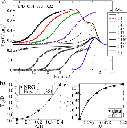
Figure 7: (Color online) a) Temperature-dependent susceptibility of the $2$-dot system with unequal (detuned) on-site energies, $\delta_{1}=\Delta$, $\delta_{2}=-\Delta$. Full symbols present Bethe-Ansatz results of the equivalent $S=1$ Kondo model, while empty symbols are BA results of a $S=1/2$ Kondo model. b) Comparison of calculated and predicted Kondo temperature, see Eqs. (5) and  (38). c) The Kondo temperature of the S=1/2 Kondo screening on the singlet side of the transition and a fit to Eq. (39).

Even though the two dots are now inequivalent, the Schrieffer-Wolff transformation yields the same $J_{K}$ for both spin impurities. We obtain

$$J_{K}=2|V_{k_{F}}|^{2}\left(\frac{1}{|\Delta-U/2|}+\frac{1}{|\Delta+U/2|}\right).$$ (38)

Due to the particle-hole symmetry no potential scattering is generated. The effective Kondo Hamiltonian for small $\Delta$ is thus nearly the same as that for small $\delta$ discussed in the previous section. In Fig. 7b calculated Kondo temperatures are plotted in comparison with analytical result from Eqs. (5) and (38). The agreement is excellent.

The properties of the systems with $\delta\neq 0$ and $\Delta\neq 0$ become markedly different near respective singlet-triplet transition points. For $\delta\neq 0$, the transition is induced by charge fluctuations which suppress magnetic ordering and, due to equal coupling of both dots to the band, the transition is of first order. For $\Delta\neq 0$ the transition is induced by depopulating dot 2 and populating dot 1 while the total charge on the dots is maintained, which leads to the transition from an inter-impurity triplet to a local spin-singlet on the dot 1. Since there is an asymmetry between the dots, the transition is of the Kosterlitz-Thouless type Vojta et al. (2002).

The Kondo temperature of the $S=1/2$ Kondo screening near the transition on the singlet side, $T^{*}$, is approximately given by

$$\log{T^{*}/D}=-\alpha-\beta\exp\left(-\frac{\Delta-{\tilde{\Delta}}}{\lambda}\right).$$ (39)

We obtain $\alpha\approx 7$, $\beta\approx 2.8$, ${\tilde{\Delta}}/D\approx 0.477$ and $\lambda/D\approx 1.5\times 10^{-3}$. This expression is consistent with the cross-over scale formula $T^{*}\propto\exp[-T_{K}/J_{12}]$ for a system of two fictitious spins, one directly coupled to the conduction band and the other side-coupled to the first one with exchange-interaction $J_{12}$ that depends exponentially on $\Delta$: $J_{12}=T_{K}/\beta\exp[(\Delta-{\tilde{\Delta}})/\lambda]$.

VI.2 Inter-impurity interaction

VI.2.1 Inter-impurity exchange interaction

In this subsection we show that by introducing an explicit exchange interaction $J_{12}$ between the localized spins on the dots, the strength of the RKKY interaction, $J_{\mathrm{RKKY}}$, can be directly determined. We thus study the two-impurity Anderson model with

$$H_{\mathrm{dots}}=\sum_{i=1}^{2}H_{\mathrm{dot},i}+J_{12}\boldsymbol{S}_{1}\cdot\boldsymbol{S}_{2},$$

where $J_{12}>0$.

As seen from Fig. 8, for $J_{12}$ above a critical value $J_{c}$, the RKKY interaction is compensated, local moments on the dots form the singlet rather than the triplet which in turn prevents formation of the $S=1$ Kondo effect. The phase transition is of the first order Vojta et al. (2002). Using Eq. (32), we obtain $T_{F}^{*}/D\approx 1.87\times 10^{-5}$ for the non-perturbed problem with the same $U$ and $\Gamma$, while $J_{c}/D\approx 1.68\times 10^{-5}$. Taking into account the definition $T_{F}^{*}=J_{\mathrm{RKKY}}/\beta$, where $\beta\sim 1$, we conclude that $J_{\mathrm{RKKY}}$ agrees well with the critical value of $J_{c}$, i.e. $J_{c}=J_{\mathrm{RKKY}}$. The perturbation theory prediction of $J_{\mathrm{RKKY}}/D=1.6\times 10^{-5}$ also agrees favorably with numerical results.

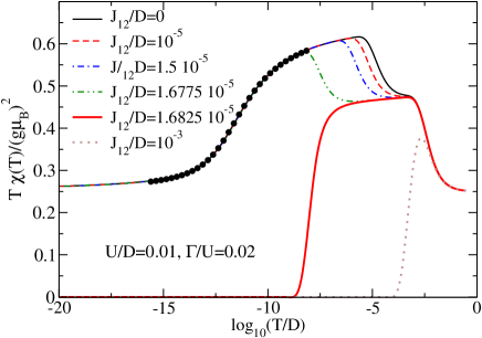
Figure 8: (Color online) Temperature-dependent susceptibility of the 2-dot systems for different anti-ferromagnetic inter-impurity couplings $J_{12}$. Circles are Bethe-Ansatz results for the susceptibility of the $S=1$ Kondo model with the Kondo temperature which is equal for all cases where $J_{12}<J_{\mathrm{c}}$.

As long as $J_{12}<J_{c}$, even for $J_{12}>T_{K}$, the $S=1$ Kondo effect survives and, moreover, the Kondo temperature remains unchanged, determined only by the value of $\rho_{0}J_{\mathrm{K}}$ as in the $J_{12}=0$ case. The only effect of increasing $J_{12}$ in the regime where $J_{12}<J_{\mathrm{c}}$ is the reduction of the transition temperature into the triplet state, which is now given by $T_{F}^{*}\sim J_{\mathrm{eff}}/\beta$ with the effective inter-impurity interaction $J_{\mathrm{eff}}=J_{\mathrm{RKKY}}-J_{12}$.

VI.2.2 Hopping between the impurities

We now study the two-impurity Anderson model with additional hopping between the dots:

$$H_{\mathrm{dots}}=\sum_{i=1}^{2}H_{dot,i}-t_{12}\sum_{\sigma}\left(d^{\dagger}_{1\sigma}d_{2\sigma}+d^{\dagger}_{2\sigma}d_{1\sigma}\right),$$ (40)

This model can be viewed also as a single-channel version of the Alexander-Anderson model Alexander and Anderson (1964) in the limit of zero separation between the impurities. The magnetic-susceptibility curves are shown in Fig. 9.

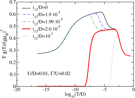
Figure 9: (Color online) Temperature-dependent susceptibility of the 2-dot systems with inter-dot tunneling coupling $t_{12}$. For $t_{12}/D\approx 2\times 10^{-4}$, we have $J_{\mathrm{AFM}}/D\approx 1.6\times 10^{-5}$, which agrees well with the critical value of $J_{c}/D\approx 1.7\times 10^{-5}$ found in the case of an explicit exchange interaction between the dots, see Fig. 8.

The hopping leads to hybridization between the atomic levels of the dots which in turn results in the formation of an even and odd level (“molecular orbital”) with energies $\epsilon_{e,o}=\epsilon_{d}\pm t_{12}$. In the presence of interaction $U$ there are two contributions to the energy of the low-lying states: “orbital energy” proportional to $t_{12}$ and “magnetic energy” due to an effective antiferromagnetic exchange $J_{\mathrm{AFM}}=4t_{\mathrm{12}}^{2}/U$, which is second-order in $t_{12}$. Even though the orbital energy is the larger energy scale, the Kondo effect is largely insensitive to the resulting level splitting. Instead, the Kondo effect is destroyed when $J_{\mathrm{AFM}}$ exceeds $J_{\mathrm{RKKY}}$, much like in the case of explicit exchange interaction between the dots which was discussed in the previous subsection. We should emphasize the similarity between the curves in Figs. 8 and 9.

In the wide-band limit $U\ll D$, $J_{\mathrm{RKKY}}/D\approx 0.62\times 16V^{4}/U$, therefore the critical $t_{12,c}$ is given by $t_{12,c}\approx\Gamma$ and it does not depend on $U$. This provides an alternative interpretation for the $U$-dependence of $t_{12,c}$ in the strong-coupling regime found in Ref. Nishimoto et al., 2006.

VI.3 Isospin-invariance breaking perturbations

The inter-impurity electron repulsion and the two-electron hopping between the impurities represent perturbations that break the isospin $SU(2)$ symmetry of the original model, while they preserve both the particle-hole symmetry as well as the spin invariance.

VI.3.1 Inter-impurity electron repulsion

The effect of the inter-impurity electron repulsion (induced by capacitive coupling between the two parallel quantum dots) is studied using the Hamiltonian

$$H_{\mathrm{dots}}=\sum_{i=1}^{2}H_{dot,i}+U_{12}(n_{1}-1)(n_{2}-1),$$ (41)

where it should be noted that $(n_{1}-1)(n_{2}-1)=4I_{1}^{z}I_{2}^{z}$ is the longitudinal part of the isospin-isospin exchange interaction $\boldsymbol{I}_{1}\cdot\boldsymbol{I}_{2}$.

Results in Fig. 10 show that the inter-impurity repulsion is not an important perturbation as long as $U_{12}<U$. Finite $U_{12}$ only modifies the Kondo temperature and the temperature $T_{1}^{*}$ of the FO-LM transition, while the behavior of the system remains qualitatively unchanged. Note that $T_{F}^{*}$ is unchanged since $U_{12}$ equally affects both the singlet and the triplet energy.

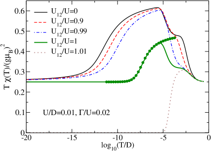
Figure 10: (Color online) Temperature-dependent susceptibility of the 2-dot systems for different inter-impurity electron-electron repulsion parameters $U_{12}$. Circles are the Bethe-Ansatz results for the $S=1/2$ Kondo model which fit the NRG results in the special case $U_{12}=U$.

For $U_{12}>U$ the electrons can lower their energy by forming on-site singlets and the system enters the charge-ordering regime Galpin et al. (2005). This behavior bares some resemblance to that of the negative-$U$ Anderson model Taraphder and Coleman (1991) which undergoes a charge Kondo effect.

The system behaves in a peculiar way at the transition point $U_{12}=U$ where $U_{12}$ and $U$ terms can be combined using isospin operators as

$$U/2\left(4(I_{1}^{z})^{2}+4(I_{2}^{z})^{2}\right)+U_{12}4I_{1}^{z}I_{2}^{z}=2U(I^{z})^{2}.$$ (42)

We now have an intermediate temperature fixed point with a six-fold symmetry of states with $I_{z}=0$ as can be deduced from Eq. (42) and the entropy curve in Fig. 11.

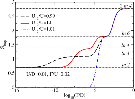
Figure 11: (Color online) Temperature-dependent entropy of the 2-dot systems for different inter-impurity electron-electron repulsion $U_{12}$.

For two impurities we can define an orbital pseudo-spin operator as

$$\boldsymbol{O}=\frac{1}{2}\sum_{\alpha}\sum_{i,j=1,2}d^{\dagger}_{i\alpha}\boldsymbol{\sigma}_{ij}d_{j\alpha},$$ (43)

where $\boldsymbol{\sigma}$ is the vector of the Pauli matrices. The quantum dots Hamiltonian $H_{\mathrm{dots}}$ commutes for $U_{12}=U$ with all three components of the orbital pseudo-spin operator; the decoupled impurities thus have orbital $SU(2)_{\mathrm{orb}}$ symmetry. Furthermore, pseudo-spin $\boldsymbol{O}$ and spin $\boldsymbol{S}$ operators commute and the symmetry is larger, $SU(2)_{\mathrm{spin}}\otimes SU(2)_{\mathrm{orb}}$. In fact, the set of three $S^{i}$, three $O^{i}$ and nine operators $S^{i}O^{j}$ are the generators of the $SU(4)$ symmetry group of which $SU(2)_{\mathrm{spin}}\otimes SU(2)_{\mathrm{orb}}$ is a subgroup. The six degenerate states are the spin triplet, orbital singlet and the spin singlet, orbital triplet Leo and Fabrizio (2004) which form a $SU(4)$ sextet:

$$\begin{split}|S=1,S_{z}=1,O=0\rangle&=|\uparrow,\uparrow\rangle,\\ |S=1,S_{z}=0,O=0\rangle&=1/\sqrt{2}\left(|\uparrow,\downarrow\rangle+|\downarrow,\uparrow\rangle\right),\\ |S=1,S_{z}=-1,O=0\rangle&=|\downarrow,\downarrow\rangle,\\ |S=0,O=1,O_{z}=1\rangle&=|\uparrow\downarrow,0\rangle,\\ |S=0,O=1,O_{z}=0\rangle&=1/\sqrt{2}\left(|\uparrow,\downarrow\rangle-|\downarrow,\uparrow\rangle\right),\\ |S=0,O=1,O_{z}=-1\rangle&=|0,\uparrow\downarrow\rangle.\end{split}$$

The states $|S=0,O=1,O_{z}=\pm 1\rangle$ can be combined into an isospin triplet $|S=0,I=1,I_{z}=0\rangle=1/\sqrt{2}\left(|\uparrow\downarrow,0\rangle+|0,\uparrow\downarrow\rangle\right)$ and an isospin singlet $|S=0,I=0\rangle=1/\sqrt{2}\left(|\uparrow\downarrow,0\rangle-|0,\uparrow\downarrow\rangle\right)$.

The coupling of impurities to the leads, however, breaks the orbital symmetry. Unlike the model studied in Ref. Galpin et al., 2005, our total Hamiltonian $H$ is not $SU(4)$ symmetric, so no $SU(4)$ Kondo effect is expected. Instead, as the temperature decreases the degeneracy first drops from 6 to 4 and then from 4 to 2 in a $S=1/2$ $SU(2)$ Kondo effect (see the fit to the Bethe-Ansatz result in Fig. 10). There is a residual two-fold degeneracy in the ground state. To understand these results, we applied perturbation theory (Appendix A) which shows that the sextuplet splits in the fourth order perturbation in $V_{k}$. The spin-triplet states and the state $|S=0,I=0\rangle$ form the new four-fold degenerate low-energy subset of states, while the states $|S=0,I=1,I_{z}=0\rangle$ and $|S=0,O=1,O_{z}=0\rangle$ have higher energy. The remaining four states can be expressed in terms of even and odd molecular-orbitals described by operators $d_{e\sigma}^{\dagger}=1/\sqrt{2}\left(d^{\dagger}_{1\sigma}+d^{\dagger}_{2\sigma}\right)$ and $d_{o\sigma}^{\dagger}=1/\sqrt{2}\left(d^{\dagger}_{1\sigma}-d^{\dagger}_{2\sigma}\right)$. We obtain

$$\begin{split}|S=1,S_{z}=1,O=0\rangle&=d^{\dagger}_{e,\uparrow}d^{\dagger}_{o,\uparrow}|0\rangle,\\ |S=1,S_{z}=0,O=0\rangle&=1/\sqrt{2}\left(d^{\dagger}_{o,\uparrow}d^{\dagger}_{e,\downarrow}+d^{\dagger}_{e,\uparrow}d^{\dagger}_{o,\downarrow}\right)|0\rangle,\\ |S=1,S_{z}=-1,O=0\rangle&=d^{\dagger}_{e,\downarrow}d^{\dagger}_{o,\downarrow}|0\rangle,\\ |S=0,I=0\rangle&=1/\sqrt{2}\left(d^{\dagger}_{o,\uparrow}d^{\dagger}_{e,\downarrow}-d^{\dagger}_{e,\uparrow}d^{\dagger}_{o,\downarrow}\right)|0\rangle.\end{split}$$ (44)

The four remaining states are therefore a product of a spin-doublet in the even orbital and a spin-doublet in the odd orbital. Due to the symmetry of our problem, only the even orbital couples to the leads, while the odd orbital is entirely decoupled. The electron in the even orbital undergoes $S=1/2$ Kondo screening, while the unscreened electron in the odd orbital is responsible for the residual two-fold degeneracy.

VI.3.2 Two-electron hopping

We consider the Hamiltonian

$$H_{\mathrm{dots}}=\sum_{i=1}^{2}H_{dot,i}-T_{12}\hat{T},$$ (45)

where $\hat{T}$ is the two-electron hopping operator that can be expressed in terms of the transverse part of the isospin-isospin exchange interaction $\boldsymbol{I}_{1}\cdot\boldsymbol{I}_{2}$:

$$\begin{split}\hat{T}&=d^{\dagger}_{1\uparrow}d^{\dagger}_{1\downarrow}d_{2\downarrow}d_{2\uparrow}+d^{\dagger}_{2\uparrow}d^{\dagger}_{2\downarrow}d_{1\downarrow}d_{1\uparrow}\\ &=I_{1}^{+}I_{2}^{-}+I_{1}^{-}I_{2}^{+}=2(I_{1}^{x}I_{2}^{x}+I_{1}^{y}I_{2}^{y}).\end{split}$$ (46)

This perturbation term is complementary to the one generated by $U_{12}$ in Eq. (42) and studied in the previous subsection. Physically, it corresponds to correlated tunneling of electron pairs which can be neglected in the applications to problems of transport through parallel quantum dots coupled electrostatically as physically realized in semiconductor heterostructures. Models featuring pair-tunneling terms as in Eq. (46) may, however, be of interest to problems in tunneling through molecules with vibrational degrees of freedom, where ground states with even number of electrons can be favored due to a polaronic energy shift Mravlje et al. (2005); Koch et al. (2006). In such cases, the charge transport is expected to be dominated by the electron-pair tunneling Koch et al. (2006).

The temperature dependence of the magnetic susceptibility shown in Fig. 12 again demonstrates the robustness of the $S=1$ state for $|T_{12}|<U$. The behavior of the system for negative $T_{12}$ is similar to the case of the inter-impurity repulsion. For $T_{12}=-U$ we again observe special behavior of the susceptibility curve, characteristic for the six-fold degeneracy observed in the previous subsection at $U_{12}=U$. For positive $T_{12}$ the system undergoes the $S=1$ spin Kondo effect up to and including $T_{12}=U$. The FO-LM transition temperature $T_{1}^{*}$ and the Kondo temperature are largely $T_{12}$ independent, while the LM-FF transition temperature $T_{F}^{*}$ decreases with increasing $T_{12}$.

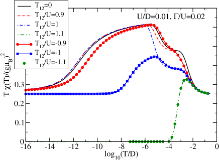
Figure 12: (Color online) Temperature-dependent susceptibility of the $2$-dot system with two-electron hopping between the dots $T_{12}$.

VI.4 Unequal coupling to the continuum

We finally study the Hamiltonian that allows for unequal hybridizations $\Gamma_{i}=\pi\rho_{0}|V^{i}_{k_{F}}|^{2}$ in the following form:

$$H=H_{\mathrm{band}}+H_{\mathrm{dots}}+\sum_{i=1}^{2}H_{\mathrm{c},i},$$ (47)

with

$$H_{\mathrm{c},i}=\frac{1}{\sqrt{L}}\sum_{k\sigma}\left(V_{k}^{i}d^{\dagger}_{i\sigma}c_{k\sigma}+\text{H.c.}\right).$$ (48)

We set $V^{2}_{k}=\alpha V^{1}_{k}$, i.e. $\Gamma_{2}=\alpha^{2}\Gamma_{1}$.

The effective low-temperature Hamiltonian can be now written as

$$H_{\mathrm{eff}}=H_{\mathrm{band}}+\boldsymbol{s}\cdot\sum_{i=1}^{2}J_{\mathrm{K},i}\boldsymbol{S}_{i}-J^{\mathrm{eff}}_{\mathrm{RKKY}}\boldsymbol{S}_{1}\cdot\boldsymbol{S}_{2}.$$ (49)

with $J_{K,2}=\alpha^{2}J_{K,1}$ and with the effective RKKY exchange interaction given by a generalisation of Eq. (21)

$$J^{\mathrm{eff}}_{\mathrm{RKKY}}=0.62U\rho_{0}^{2}J_{\mathrm{K},1}J_{\mathrm{K,2}}=\alpha^{2}J_{\mathrm{RKKY}},$$ (50)

where $J_{\mathrm{RKKY}}$ is the value of RKKY parameter at $\alpha=1$. In our attempt to derive the effective Hamiltonian we assume that in the temperature regime $T\lesssim J^{\mathrm{eff}}_{\mathrm{RKKY}}$ the two moments couple into a triplet. Since the two Kondo exchange constants $J_{\mathrm{K},i}$ are now different, we rewrite $H_{\mathrm{eff}}$ in Eq. (49) in the following form

$$\begin{split}H_{\mathrm{eff}}=H_{\mathrm{band}}&+\boldsymbol{s}\cdot\left(\frac{J_{\mathrm{K},1}+J_{\mathrm{K},2}}{2}\left(\boldsymbol{S}_{1}+\boldsymbol{S}_{2}\right)\right)\\ &+\boldsymbol{s}\cdot\left(\frac{J_{\mathrm{K},1}-J_{\mathrm{K},2}}{2}\left(\boldsymbol{S}_{1}-\boldsymbol{S}_{2}\right)\right)\\ &-J^{\mathrm{eff}}_{\mathrm{RKKY}}\boldsymbol{S}_{1}\cdot\boldsymbol{S}_{2}.\end{split}$$ (51)

Within the triplet subspace, $\boldsymbol{S}_{1}+\boldsymbol{S}_{2}$ is equal to the new composite spin 1, which we denote by $\boldsymbol{S}$, $\boldsymbol{S}_{1}-\boldsymbol{S}_{2}$ is identically equal to zero, and $\boldsymbol{S}_{1}\cdot\boldsymbol{S}_{2}$ is a constant $-1/4$. As a result, the effective $J_{\mathrm{K}}$ is simply the average of the two exchange constants:

$$J_{\mathrm{K},\mathrm{eff}}=\frac{J_{\mathrm{K},1}+J_{\mathrm{K},2}}{2}.$$ (52)

Susceptibility curves for different $\alpha$ are shown in Fig. 13. Note that the Kondo temperature determined using Eq. (5) combined with the naive argument given in Eq. (52) fails to describe the actual Kondo scale for $\alpha\lesssim 0.4$ as seen from Fig. 14. This is due to admixture of the singlet state, which also renormalizes $J_{K}$, even though the singlet is separated by $J^{\mathrm{eff}}_{\mathrm{RKKY}}\gg T_{K}$ from the triplet subspace. Note however, that $J^{\mathrm{eff}}_{\mathrm{RKKY}}$ is well described by the simple expression given in Eq. (50) as shown in Fig. 14. By performing a second-order RG calculation (see Appendix B), which takes the admixture of the singlet state into account, we obtain $T_{K}$ as a function of $\alpha$ which agrees very well with the NRG results, see Fig. 14.

For extremely small $\alpha$, $J^{\mathrm{eff}}_{\mathrm{RKKY}}$ eventually becomes comparable to the Kondo temperature, see Fig. 14. For that reason the ferromagnetic locking-in is destroyed and the system behaves as a double $S=1/2$ doublet, one of which is screened at $T_{K}^{1}=T_{K}(J_{\mathrm{K,1}})$ as shown in Fig. 13b.

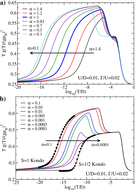
Figure 13: (Color online) Temperature-dependent susceptibility of the $2$-dot system with unequal coupling to the leads, $\Gamma_{2}=\alpha^{2}\Gamma_{1}$. a) The range of $\alpha$ where $T_{K}$ is decreasing. b) The range of $\alpha$ where $T_{K}$ is increasing again. Circles (squares) are BA results for the $S=1$ ($S=1/2$) Kondo model. The arrows indicate the evolution of the susceptibility curves as the parameter $\alpha$ decreases.

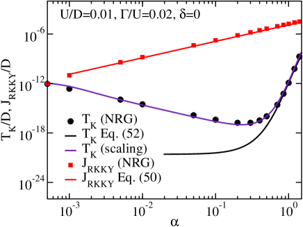
Figure 14: (Color online) Comparison of calculated and predicted Kondo temperature $T_{K}$ and effective exchange interaction $J^{\mathrm{eff}}_{\mathrm{RKKY}}$. The calculation of scaling results for $T_{K}$ is described in Appendix B.

VII Conclusions

We have shown that several magnetic impurities, coupled to the same Wannier orbital of a conduction electron band, experience ferromagnetic RKKY interaction which locks local moments in a state of a maximal total spin. The multi-impurity Anderson model is at low temperatures, i.e. for $T<T_{F}^{*}$, equivalent to a $S=N/2$ $SU(2)$ Kondo model. Using perturbation theory up to the fourth order in $V$ we derived an analytical expression for $J_{\mathrm{RKKY}}$ and tested it against NRG calculations. We have also shown that the high-spin state is very robust against experimentally relevant perturbations such as particle-hole symmetry breaking, on-site energy level splitting, inter-impurity capacitive coupling and direct exchange interaction. At low temperatures, the ferromagnetically locked impurities undergo a collective Kondo cross-over in which half of a unit of spin is screened. The Kondo temperature in this simple model does not depend on the total spin (i.e. on the number of impurities $N$), while the LM-FF temperature $T_{F}^{*}$ is weakly $N$-dependent.

We next list a few most important findings concerning the effect of various perturbations to the original two-dot system: a) $T_{F}^{*}$ is in the range $\delta\lesssim 0.4U$ nearly independent of the deviation from the particle-hole symmetric point $\delta=0$, b) increasing the difference between on-site energies of two dots, $2\Delta$, induces a Kosterlitz-Thouless type phase transition separating the phase with $S=1/2$ residual spin at low-temperatures from the $S=0$ one, c) introduction of additional one-electron hopping between the impurities induces effective AFM interaction $J_{\mathrm{AFM}}=4t_{12}^{2}/U$ that does not effect the Kondo temperature as long as $J_{\mathrm{AFM}}\lesssim J_{\mathrm{RKKY}}$, nevertheless, at $t_{12}=t_{12,c}$ it destabilizes the $S=1$ state. The critical value $t_{12,c}\sim\Gamma$ does not depend on $U$, d) inter-impurity Coulomb interaction $U_{12}$ leads to a transition from the $S=1$ Kondo state to the charge ordered state. In the 4-fold degenerate intermediate point, reached at $U_{12}=U$, the effective Hamiltonian consists of the effective $S=1/2$ Kondo model and of a free, decoupled $S=1/2$ spin, e) when the two impurities are coupled to the leads with different hybridization strengths, second-order scaling equations provide a good description of the Kondo temperature.

The properties of our model apply very generally, since high-spin states can arise whenever the RKKY interaction is ferromagnetic, even when the dots are separated in space Usaj et al. (2005); Tamura and Glazman (2005). In addition, it has become possible to study Kondo physics in clusters of magnetic atoms on metallic surfaces Jamneala et al. (2001); Aligia (2006). On (111) facets of noble metals such as copper, bulk electrons coexist with Shockley surface-state electrons Lin et al. (2005). Surface-state bands on these surfaces have $k_{F}\sim 0.1-0.2\AA^{-1}$; thus, for nearest and next-nearest neighbor adatoms $k_{F}R\lesssim 1$. If hybridization to the surface band is dominant, small clusters then effectively couple to the same Wannier orbital of the surface band and the single-channel multi-impurity Anderson model is applicable; in the absence of additional inter-impurity interactions, the spins would then tend to order ferromagnetically. If hybridization to the bulk band with $k^{3\mathrm{D}}_{F}\sim 1\AA^{-1}$ is also important, the problem must be described using a complex two-band multi-channel Hamiltonian.

Further aspects of the multi-impurity Anderson model should be addressed in the future work. Systems of coupled quantum dots and magnetic impurities on surfaces are mainly characterized by measuring their transport properties. Conductance can be determined by calculating the spectral density functions using the numerical renormalization group method. We anticipate that the fully screened $N=1$ model will have different temperature dependence as the under-screened $N\geq 2$ models. Since in quantum dots the impurity level $\delta$ (or $\epsilon_{d}$) can be controlled using gate voltages, it should be interesting to extend the study to asymmetric multi-impurity models for $N>2$ where more quantum phase transitions are expected in addition to the one already identified for $N=2$ at $\delta=\delta_{c}$.

Appendix A Rayleigh-Schroedinger perturbation theory in $V_{k}$

Following Ref. Fye, 1990, we apply Rayleigh-Schrödinger perturbation theory to calculate second and fourth order corrections in $V_{k}$ to the energy of a state $|n\rangle$:

$$\begin{split}E_{n}^{(2)}&={\sum_{m}}^{\prime}\frac{\langle n|H_{c}|m\rangle\langle m|H_{c}|n\rangle}{E_{n}-E_{m}}\\ E_{n}^{(4)}&={\sum_{m_{1},m_{2},m_{3}}}^{\prime}\\ &\frac{\langle n|H_{c}|m_{3}\rangle\langle m_{3}|H_{c}|m_{2}\rangle\langle m_{2}|H_{c}|m_{1}\rangle\langle m_{1}|H_{c}|n\rangle}{(E_{n}-E_{m_{3}})(E_{n}-E_{m_{2}})(E_{n}-E_{m_{1}})}\\ \end{split}$$ (53)

The summation extends over all intermediate states $|m_{i}\rangle$ not equal to one of the degenerate ground states. We will consider the simplified case of constant $V_{k}$, i.e. $V_{k}=V_{k_{F}}=V$.

A.1 RKKY interaction in the two-impurity case

We study the splitting between the singlet $|S\rangle=1/\sqrt{2}\left(|\uparrow,\downarrow\rangle-|\downarrow,\uparrow\rangle\right)$ and the triplet state $|T\rangle=1/\sqrt{2}\left(|\uparrow,\downarrow\rangle+|\downarrow,\uparrow\rangle\right)$. The second order corrections are $E_{S}^{(2)}=E_{T}^{(2)}=-(S_{1}+S_{2})$ with

$$\begin{split}S_{1}&=4V^{2}\frac{1}{L}\sum_{k^{\prime}\geq k_{F}}\frac{1}{U-2\delta+2\epsilon_{k^{\prime}}},\\ S_{2}&=4V^{2}\frac{1}{L}\sum_{k\leq k_{F}}\frac{1}{U+2\delta-2\epsilon_{k}}.\end{split}$$ (54)

There is therefore no splitting to this order in $V$. The fourth order corrections are

$$\begin{split}E_{S}^{(4)}&=W_{S}^{\mathrm{ph}}+W_{S}^{\mathrm{pp}}+W_{S}^{\mathrm{hh}},\\ E_{T}^{(4)}&=W_{T}^{\mathrm{ph}},\end{split}$$ (55)

where the particle-hole ($\mathrm{ph}$), particle-particle ($\mathrm{pp}$) and hole-hole ($\mathrm{hh}$) intermediate-state contributions are

$$\begin{split}W_{S}^{\mathrm{ph}}&=\frac{16V^{4}}{U}\frac{1}{L^{2}}\sum_{k\leq k_{F},k^{\prime}>k_{F}}\frac{8(\delta-\epsilon_{k})(\delta-\epsilon_{k^{\prime}})(U+\epsilon_{k}-\epsilon_{k^{\prime}})}{(U-2\delta+2\epsilon_{k})^{2}(U+2\delta-2\epsilon_{k^{\prime}})^{2}(\epsilon_{k}-\epsilon_{k^{\prime}})},\\ W_{T}^{\mathrm{ph}}&=32V^{4}\frac{1}{L^{2}}\sum_{k\leq k_{F},k^{\prime}>k_{F}}\frac{2U^{2}+5U(\epsilon_{k}-\epsilon_{k^{\prime}})+4\left(\delta^{2}+\epsilon_{k}^{2}+\epsilon_{k^{\prime}}^{2}-\epsilon_{k}\epsilon_{k^{\prime}}-\delta(\epsilon_{k}+\epsilon_{k^{\prime}})\right)}{(U-2\delta+2\epsilon_{k})^{2}(U+2\delta-2\epsilon_{k^{\prime}})^{2}(\epsilon_{k}-\epsilon_{k^{\prime}})},\\ W_{S}^{\mathrm{pp}}&=\frac{16V^{4}}{U}\frac{1}{L^{2}}\sum_{k^{\prime}_{1}>k_{F},k^{\prime}_{2}>k_{F}}\frac{2(U-2\delta)(3U-2\delta)+8(U-\delta)(\epsilon_{k^{\prime}_{1}}+\epsilon_{k^{\prime}_{2}})+8\epsilon_{k^{\prime}_{1}}\epsilon_{k^{\prime}_{2}}}{(U-2\delta+2\epsilon_{k^{\prime}_{1}})^{2}(U-2\delta+2\epsilon_{k^{\prime}_{2}})^{2}},\\ W_{S}^{\mathrm{hh}}&=\frac{16V^{4}}{U}\frac{1}{L^{2}}\sum_{k_{1}\leq k_{F},k_{2}\leq k_{F}}\frac{2(U+2\delta)(3U+2\delta)-8(U+\delta)(\epsilon_{k_{1}}+\epsilon_{k_{2}})+8\epsilon_{k_{1}}\epsilon_{k_{2}}}{(U+2\delta-2\epsilon_{k_{1}})^{2}(U+2\delta-2\epsilon_{k_{2}})^{2}}.\end{split}$$ (56)

From these expressions we obtain $J_{\mathrm{RKKY}}=E_{S}-E_{T}$. In order to evaluate the sums for a flat band with a constant density of states $\rho_{0}=1/(2D)$ and the chemical potential $\mu=0$, we make formal replacements $\frac{1}{L}\sum_{k^{\prime}>k_{F}}=\frac{1}{L}\sum_{k^{\prime}>0}\to 1/2\int_{0}^{1}dk^{\prime}$ and $\frac{1}{L}\sum_{k\leq k_{F}}=\frac{1}{L}\sum_{k<=0}\to 1/2\int_{-1}^{0}dk$. In Fig. 15 we plot the prefactor $c$ in the expression for the exchange constant $J_{\mathrm{RKKY}}=c16V^{4}/U$ as a function of $U/D$. In the wide-band limit, i.e. for small $U/D$, $c$ approaches a constant value of $c=0.616$ irrespective of the value of $\delta/U$. The dependence of $c$ on $\delta$ for $U/D\sim 1$ is due to the band-edge effects.

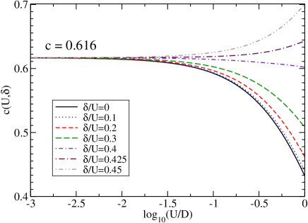
Figure 15: The prefactor $c$ in the RKKY exchange constant $J_{\mathrm{RKKY}}=c16V^{4}/U$ for a flat band with $\rho_{0}=1/(2D)$ as a function of $U$ for a range of values of the impurity energy level $\delta$.

To determine the temperature $T_{J}$ at which the RKKY interaction becomes fully established, we calculate the cut-off dependent $J_{\mathrm{RKKY}}(E)$, where $E$ is the low-energy cut-off for $k$ and $k^{\prime}$ integrations, i.e. the integrals over $k$ and $k^{\prime}$ become $\int_{E}^{1}dk^{\prime}$ and $\int_{-1}^{-E}dk$. In Fig. 16 we plot the ratio $\xi(E)=J_{\mathrm{RKKY}}(E)/J_{\mathrm{RKKY}}^{0}$, where $J_{\mathrm{RKKY}}^{0}=J_{\mathrm{RKKY}}(E\to 0)$. The ratio $\xi(E)$ reaches an (arbitrarily chosen) value of $0.9$ at $E/U\sim 0.02$. This value of $E$ roughly defines $T_{J}$ below which the RKKY is fully developed. For small enough $V$ (i.e. $\Gamma$), the value of $T_{J}$ is positioned between $T_{1}^{*}$ (free-orbital to local-moment transition temperature) and $T_{F}^{*}$, the temperature of ferromagnetic ordering of spins, given by $T_{F}^{*}=J_{\mathrm{RKKY}}^{0}/\beta$, where $\beta$ is a constant of the order one. For larger $V$, however, $J_{\mathrm{RKKY}}(T)$ does not reach its limiting value at the temperature where the spins start to order. In this case we obtain the ordering temperature $T_{F}^{*}$ numerically as the solution of the implicit equation

$$T_{F}^{*}=J_{\mathrm{RKKY}}(T_{F}^{*})/\beta.$$ (57)

An approximate fit to $\xi(E)$ in the wide-band limit is $\xi(E)=1/(1+xE/U)$ with $x=12.2$. We then obtain a solution for $T_{F}^{*}$ in closed form:

$$\begin{split}T_{F}^{*}&=\frac{\sqrt{1+4x/\beta(J_{\mathrm{RKKY}}^{0}/U)}-1}{2x/U}\\ &\approx\frac{J^{0}_{\mathrm{RKKY}}}{\beta}\left(1-\frac{x}{\beta}\frac{J_{\mathrm{RKKY}}^{0}}{U}+{\mathcal{O}}\left(\frac{J_{\mathrm{RKKY}}^{0}}{U}\right)^{2}\right).\end{split}$$ (58)

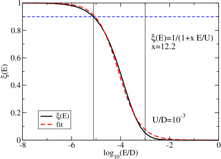
Figure 16: Ratio $\xi(E)=J_{\mathrm{RKKY}}(E)/J_{\mathrm{RKKY}}^{0}$ of the running RKKY coupling constant at energy $E$ over its value in the $E\to 0$ limit. The dashed line is an approximate fit to a simple rational function $\xi(E)=1/(1+xE/U)$.

A.2 Six-fold symmetric $U_{12}=U$ case

We study the splitting between the singlet, the triplet (same as above) and the “exciton” states $|I=0\rangle=1/\sqrt{2}\left(|\uparrow\downarrow,0\rangle-|0,\uparrow\downarrow\rangle\right)$ and $|I=1\rangle=1/\sqrt{2}\left(|\uparrow\downarrow,0\rangle+|0,\uparrow\downarrow\rangle\right)$. Second order corrections are all equal: $E_{S}^{(2)}=E_{T}^{(2)}=E_{I=0}^{(2)}=E_{I=1}^{(2)}=-(S_{1}+S_{2})$ where $S_{1}$ and $S_{2}$ are the same as in the previously treated $U_{12}=0$ case. There is again no splitting to second order in $V$. The fourth order corrections are

$$\begin{split}E_{S}^{(4)}&=W_{S}^{\mathrm{ph}}+W_{S}^{\mathrm{pp}}+W_{S}^{\mathrm{hh}}\\ E_{T}^{(4)}&=W_{T}^{\mathrm{ph}}\\ E_{I=0}^{(4)}&=E_{T}^{(4)}\\ E_{I=1}^{(4)}&=E_{S}^{(4)}\end{split}$$ (59)

where

$$\begin{split}W_{S}^{\mathrm{ph}}&=16V^{4}\frac{1}{L^{2}}\sum_{k\leq k_{F},k^{\prime}>k_{F}}\frac{1}{\epsilon_{k}-\epsilon_{k^{\prime}}}\left(\frac{1}{(U-2\delta+2\epsilon_{k})^{2}}+\frac{1}{(U+2\delta-2\epsilon_{k^{\prime}})^{2}}\right),\\ W_{T}^{\mathrm{ph}}&=32V^{4}\frac{1}{L^{2}}\sum_{k\leq k_{F},k^{\prime}>k_{F}}\frac{3U^{2}+6U(\epsilon_{k}-\epsilon_{k^{\prime}})+4\left(\delta^{2}+\epsilon_{k}^{2}+\epsilon_{k^{\prime}}^{2}-\epsilon_{k}\epsilon_{k^{\prime}}-\delta(\epsilon_{k}+\epsilon_{k^{\prime}})\right)}{(U-2\delta+2\epsilon_{k})^{2}(U+2\delta-2\epsilon_{k})^{2}(\epsilon_{k}-\epsilon_{k^{\prime}})},\\ W_{S}^{\mathrm{pp}}&=16V^{4}\frac{1}{L^{2}}\sum_{k^{\prime}_{1}>k_{F},k^{\prime}_{2}>k_{F}}\frac{2(U-2\delta+\epsilon_{k^{\prime}_{1}}+\epsilon_{k^{\prime}_{2}})^{2}}{(U-2\delta+2\epsilon_{k^{\prime}_{1}})^{2}(U-2\delta+2\epsilon_{k^{\prime}_{2}})^{2}(2U-2\delta+\epsilon_{k^{\prime}_{1}}+\epsilon_{k^{\prime}_{2}})},\\ W_{S}^{\mathrm{hh}}&=16V^{4}\frac{1}{L^{2}}\sum_{k_{1}\leq k_{F},k_{2}\leq k_{F}}\frac{2(U+2\delta-\epsilon_{k_{1}}+\epsilon_{k_{2}})^{2}}{(U+2\delta-2\epsilon_{k_{1}})^{2}(U+2\delta-2\epsilon_{k_{2}})(2U+2\delta-\epsilon_{k_{1}}+\epsilon_{k_{2}})}.\end{split}$$ (60)

The triplet is degenerate with the $I=0$ state, while the singlet and the $I=1$ state are higher in energy, as determined by performing the integrations (results not shown).

Appendix B Scaling equations to second order in $J$

We consider an effective Hamiltonian of the form

$$\begin{split}H&=\sum_{k\sigma}\epsilon_{k}c^{\dagger}_{k\sigma}c_{k\sigma}+\sum_{m}E_{m}X_{mm}\\ &+\sum_{mm^{\prime},kk^{\prime},\sigma\sigma^{\prime}}J^{\sigma\sigma^{\prime}}_{mm^{\prime}}X_{mm^{\prime}}c^{\dagger}_{k\sigma}c_{k^{\prime}\sigma^{\prime}},\end{split}$$ (61)

where $X_{mm^{\prime}}=|m\rangle\langle m^{\prime}|$ are the Hubbard operators and $J^{\sigma\sigma^{\prime}}_{mm^{\prime}}$ are generalized exchange constants.

We write Hewson (1993)

$$\begin{split}&\Bigl{[}H_{11}+H_{12}\left(E-H_{22}\right)^{-1}H_{21}\\ &+H_{10}\left(E-H_{00}\right)^{-1}H_{01}\Bigr{]}\psi_{1}=E\psi_{1},\end{split}$$ (62)

where subspaces 2 corresponds to states with one electron in the upper $|\delta D|$ edge of the conduction band, 0 corresponds to states with one hole in the lower $|\delta D|$ edge of the band, and 1 corresponds to states with no excitations in the edges that are being traced-over. Furthermore, $H_{ij}=P_{i}HP_{j}$, where $P_{i}$ are projectors to the corresponding subspaces $i$.

To second order, the coupling constant are changed by

$$\begin{split}\delta J^{\sigma\sigma^{\prime}}_{mm^{\prime}}&=\rho_{0}|\delta D|\sum_{n\tau}\frac{1}{E-D+\epsilon_{k}-E_{n}-H_{0}}J^{\tau\sigma}_{nm}J^{\tau\sigma^{\prime}}_{nm^{\prime}}\\ &-\rho_{0}|\delta D|\sum_{n\tau}\frac{1}{E-D-\epsilon_{k^{\prime}}-E_{n}-H_{0}}J^{\sigma^{\prime}\tau}_{nm}J^{\sigma\tau}_{nm^{\prime}}.\\ \end{split}$$ (63)

We apply these results to the effective low-temperature Kondo Hamiltonian

$$H_{\mathrm{eff}}=H_{\mathrm{band}}+J_{1}\boldsymbol{s}\cdot\boldsymbol{S}_{1}+J_{2}\boldsymbol{s}\cdot\boldsymbol{S}_{2}-J^{\mathrm{eff}}_{\mathrm{RKKY}}\left(\boldsymbol{S}_{1}\cdot\boldsymbol{S}_{2}-1/4\right).$$ (64)

Introducing spin-1 operator $\boldsymbol{S}$ defined by the following Hubbard operator expressions: $S_{z}=X_{\uparrow\uparrow}-X_{\downarrow\downarrow}$, $S^{+}=\sqrt{2}\left(X_{\uparrow 0}+X_{0\downarrow}\right)$ and $S^{-}=(S^{+})^{\dagger}$, we obtain

$$\begin{split}H&=H_{\mathrm{band}}+{\tilde{J}}\boldsymbol{s}\cdot\boldsymbol{S}+J^{\mathrm{eff}}_{\mathrm{RKKY}}X_{SS}\\ &+\Delta\bigl{(}s_{z}(X_{0S}+X_{S0})+s^{+}(X_{\downarrow S}-X_{S\uparrow})\\ &+s^{-}(X_{S\downarrow}-X_{\uparrow S})\bigr{)},\end{split}$$ (65)

where index $S$ denotes the singlet state and we have

$$\begin{split}{\tilde{J}}&=\frac{J_{1}+J_{2}}{2}=J_{0}(1+\alpha^{2})/2,\\ \Delta&=\frac{J_{1}-J_{2}}{2}=J_{0}(1-\alpha^{2})/2.\end{split}$$ (66)

Equations (63) reduce to two equations for $\tilde{J}$ and $\Delta$

$$\begin{split}\delta{\tilde{J}}&=\rho_{0}|\delta D|\left[\frac{{\tilde{J}}^{2}}{D}+\frac{{\Delta}^{2}}{D+J^{\mathrm{eff}}_{\mathrm{RKKY}}}\right],\\ \delta\Delta&=-2\rho_{0}\frac{|\delta D|}{D}\Delta{\tilde{J}}.\end{split}$$ (67)

from which ensue the following scaling equations

$$\begin{split}\frac{d{\tilde{J}}}{dl}&=-\rho_{0}{\tilde{J}}^{2}-\rho_{0}\frac{\Delta^{2}D}{D+J^{\mathrm{eff}}_{\mathrm{RKKY}}},\\ \frac{d\Delta}{dl}&=-2\rho_{0}\Delta{\tilde{J}},\end{split}$$ (68)

where $l=\log D$. The initial bandwidth $D$ is the effective bandwidth $D_{\mathrm{eff}}=0.182U$ for the Anderson model and we take $\tilde{J}(l=\log D_{\mathrm{eff}})=\tilde{J}$ and $\Delta(l=\log D_{\mathrm{eff}})=\Delta$ with $\tilde{J}$ and $\Delta$ taken from Eq. (66). We integrate the equations numerically until $\tilde{J}$ starts to diverge. The corresponding cut-off $D$ defines the Kondo temperature. The results are shown in Fig. 14. The scaling approach reproduces our NRG results very well.

References

- Anderson (1961) P. W. Anderson, Phys. Rev. 124, 41 (1961).
- Hewson (1993) A. C. Hewson, The Kondo Problem to Heavy-Fermions (Cambridge University Press, Cambridge, 1993).
- Vladár and Zawadowski (1983) K. Vladár and A. Zawadowski, Phys. Rev. B 28, 1564 (1983).
- Madhavan et al. (1998) V. Madhavan, W. Chen, T. Jamneala, M. Crommie, and N. S. Wingreen, Science 280, 567 (1998).
- Li et al. (1998) J. Li, W.-D. Schneider, R. Berndt, and B. Delley, Phys. Rev. Lett. 80, 2893 (1998).
- Cronenwett et al. (1998) S. M. Cronenwett, T. H. Oosterkamp, and L. P. Kouwenhoven, Science 281, 540 (1998).
- Madhavan et al. (2002) V. Madhavan, T. Jamneala, K. Nagaoka, W. Chen, J.-L. Li, S. G. Louie, and M. F. Crommie, Phys. Rev. B 66, 212411 (2002).
- Jamneala et al. (2001) T. Jamneala, V. Madhavan, and M. F. Crommie, Phys. Rev. Lett. 87, 256804 (2001).
- Wahl et al. (2005) P. Wahl, L. Diekhoner, G. Wittich, L. Vitali, M. A. Schneider, and K. Kern, Phys. Rev. Lett. 95, 166601 (2005).
- Jeong et al. (2001) H. Jeong, A. M. Chang, and M. R. Melloch, Science 293, 2221 (2001).
- Holleitner et al. (2002) A. W. Holleitner, R. H. Blick, A. K. H uttel, K. Eberl, and J. P. Kotthaus, Science 297, 70 (2002).
- van der Wiel et al. (2003) W. G. van der Wiel, S. D. Franceschi, J. M. Elzerman, T. Fujisawa, S. Tarucha, and L. P. Kouwenhoven, Rev. Mod. Phys. 75, 1 (2003).
- Craig et al. (2004) N. J. Craig, J. M. Taylor, E. A. Lester, C. M. Marcus, M. P. Hanson, and A. C. Gossard, Science 304, 565 (2004).
- Chen et al. (2004) J. C. Chen, A. M. Chang, and M. R. Melloch, Phys. Rev. Lett. 92, 176801 (2004).
- Ruderman and Kittel (1954) M. A. Ruderman and C. Kittel, Phys. Rev. 96, 99 (1954).
- Jones and Varma (1987) B. A. Jones and C. M. Varma, Phys. Rev. Lett. 58, 843 (1987).
- Jones et al. (1988) B. A. Jones, C. M. Varma, and J. W. Wilkins, Phys. Rev. Lett. 61, 125 (1988).
- Jones et al. (1989) B. A. Jones, B. G. Kotliar, and A. J. Millis, Phys. Rev. B 39, 315 (1989).
- Sire et al. (1993) C. Sire, C. M. Varma, and H. R. Krishnamurthy, Phys. Rev. B 48, 13833 (1993).
- Affleck et al. (1995) I. Affleck, A. W. W. Ludwig, and B. A. Jones, Phys. Rev. B 52, 9528 (1995).
- Georges and Meir (1999) A. Georges and Y. Meir, Phys. Rev. Lett. 82, 3508 (1999).
- Izumida and Sakai (2000) W. Izumida and O. Sakai, Phys. Rev. B 62, 10260 (2000).
- Aono and Eto (2001) T. Aono and M. Eto, Phys. Rev. B 64, 073307 (2001).
- Boese et al. (2002) D. Boese, W. Hofstetter, and H. Schoeller, Phys. Rev. B 66, 125315 (2002).
- Lopez et al. (2002) R. Lopez, R. Aguado, and G. Platero, Phys. Rev. Lett. 89, 136802 (2002).
- Jayaprakash et al. (1981) C. Jayaprakash, H. R. Krishnamurthy, and J. W. Wilkins, Phys. Rev. Lett. 47, 737 (1981).
- Silva et al. (1996) J. B. Silva, W. L. C. Lima, W. C. Oliveira, J. L. N. Mello, L. N. Oliveira, and J. W. Wilkins, Phys. Rev. Lett. 76, 275 (1996).
- Paula et al. (1999) C. A. Paula, M. F. Silva, and L. N. Oliveira, Phys. Rev. B 59, 85 (1999).
- Simon et al. (2005) P. Simon, R. Lopez, and Y. Oreg, Phys. Rev. Lett. 94, 086602 (2005).
- Vavilov and Glazman (2005) M. G. Vavilov and L. I. Glazman, Phys. Rev. Lett. 94, 086805 (2005).
- Utsumi et al. (2004) Y. Utsumi, J. Martinek, P. Bruno, and H. Imamura, Phys. Rev. B 69, 155320 (2004).
- López et al. (2005) R. López, D. Sánchez, M. Lee, M.-S. Choi, P. Simon, and K. L. Hur, Phys. Rev. B 71, 115312 (2005).
- Izumida and Sakai (2005) W. Izumida and O. Sakai, J. Phys. Soc. Japan 74, 103 (2005).
- Tamura and Glazman (2005) H. Tamura and L. Glazman, Phys. Rev. B 72, 121308 (2005).
- Sasaki et al. (2000) S. Sasaki, S. de Franceschi, J. M. Elzerman, W. G. van der Wiel, M. Eto, S. Tarucha, and L. P. Kouwenhoven, Nature 405, 764 (2000).
- Izumida et al. (2001) W. Izumida, O. Sakai, and S. Tarucha, Phys. Rev. Lett. 87, 216803 (2001).
- Glazman and Raikh (1988) L. I. Glazman and M. E. Raikh, JETP Lett. 47, 452 (1988).
- Krishnamurthy et al. (1980) H. R. Krishnamurthy, J. W. Wilkins, and K. G. Wilson, Phys. Rev. B 21, 1003 (1980).
- Krishnaurthy et al. (1980) H. R. Krishnaurthy, J. W. Wilkins, and K. G. Wilson, Phys. Rev. B 21, 1044 (1980).
- Schrieffer and Wolff (1966) J. R. Schrieffer and P. A. Wolff, Phys. Rev. 149, 491 (1966).
- Wilson (1975) K. G. Wilson, Rev. Mod. Phys. 47, 773 (1975).
- Campo and Oliveira (2005) V. L. Campo and L. N. Oliveira, Phys. Rev. B 72, 104432 (2005).
- Oliveira and Oliveira (1994) W. C. Oliveira and L. N. Oliveira, Phys. Rev. B 49, 11986 (1994).
- Andrei et al. (1983) N. Andrei, K. Furuya, and J. H. Lowenstein, Rev. Mod. Phys. 55, 331 (1983).
- Rajan et al. (1982) V. T. Rajan, J. H. Lowenstein, and N. Andrei, Phys. Rev. Lett. 49, 497 (1982).
- Sacramento and Schlottmann (1989) P. D. Sacramento and P. Schlottmann, Phys. Rev. B 40, 431 (1989).
- Anderson (1970) P. W. Anderson, J. Phys. C: Solid St. Phys. 3, 2436 (1970).
- Mehta et al. (2005) P. Mehta, N. Andrei, P. Coleman, L. Borda, and G. Zarand, Phys. Rev. B 72, 014430 (2005).
- Koller et al. (2005) W. Koller, A. C. Hewson, and D. Meyer, Phys. Rev. B 72, 045117 (2005).
- Vojta et al. (2002) M. Vojta, R. Bulla, and W. Hofstetter, Phys. Rev. B 65, 140405 (2002).
- Cornaglia et al. (2004) P. S. Cornaglia, H. Ness, and D. R. Grempel, Phys. Rev. Lett. 93, 147201 (2004).
- Žitko and Bonča (2006) R. Žitko and J. Bonča, Phys. Rev. B 73, 035332 (2006).
- Hofstetter and Schoeller (2002) W. Hofstetter and H. Schoeller, Phys. Rev. Lett. 88, 016803 (2002).
- (54) R. Žitko, J. Bonča, A. Ramšak, and T. Rejec, Kondo effect in triple quantum dots, cond-mat/0601349.
- Entin-Wohlman et al. (2001) O. Entin-Wohlman, A. Aharony, and Y. Levinson, Phys. Rev. B 64, 085332 (2001).
- Fuhrer et al. (2004) A. Fuhrer, T. Ihn, K. Ensslin, W. Wegscheider, and M. Bichler, Phys. Rev. Let. 91, 206802 (2004).
- Kogan et al. (2003) A. Kogan, G. Granger, M. A. Kastner, D. Goldhaber-Gordon, and H. Shtrikman, Phys. Rev. B 67, 113309 (2003).
- Pustilnik and Glazman (2001) M. Pustilnik and L. I. Glazman, Phys. Rev. Lett. 87, 216601 (2001).
- Pustilnik et al. (2003) M. Pustilnik, L. I. Glazman, and W. Hofstetter, Phys. Rev. B 68, 161303 (2003).
- Hofstetter and Zarand (2004) W. Hofstetter and G. Zarand, Phys. Rev. B 69, 235301 (2004).
- Alexander and Anderson (1964) S. Alexander and P. W. Anderson, Phys. Rev. 133, A1594 (1964).
- Nishimoto et al. (2006) S. Nishimoto, T. Pruschke, and R. M. Noack, J. Phys.: Condens. Matter 18, 981 (2006).
- Galpin et al. (2005) M. R. Galpin, D. E. Logan, and H. R. Krishnamurthy, Phys. Rev. Lett. 94, 186406 (2005).
- Taraphder and Coleman (1991) A. Taraphder and P. Coleman, Phys. Rev. Lett. 66, 2814 (1991).
- Leo and Fabrizio (2004) L. D. Leo and M. Fabrizio, Phys. Rev. B 69, 245114 (2004).
- Mravlje et al. (2005) J. Mravlje, A. Ramšak, and T. Rejec, Phys. Rev. B 72, 121403 (2005).
- Koch et al. (2006) J. Koch, M. E. Raikh, and F. von Oppen, Phys. Rev. Lett. 96, 056803 (2006).
- Usaj et al. (2005) G. Usaj, P. Lustemberg, and C. A. Balseiro, Phys. Rev. Lett. 94, 036803 (2005).
- Aligia (2006) A. A. Aligia, Phys. Rev. Lett. 96, 096804 (2006).
- Lin et al. (2005) C.-Y. Lin, A. H. C. Neto, and B. A. Jones, Phys. Rev. B 71, 035417 (2005).
- Fye (1990) R. M. Fye, Phys. Rev. B 41, 2490 (1990).