Charged inclusion in nematic liquid crystals

Abstract

We present a general theory of liquid crystals under inhomogeneous electric field in a Ginzburg-Landau scheme. The molecular orientation can be deformed by electric field when the dielectric tensor is orientation-dependent. We then investigate the influence of a charged particle on the orientation order in a nematic state. The director is aligned either along or perpendicular to the local electric field around the charge, depending on the sign of the dielectric anisotropy. The deformation becomes stronger with increasing the ratio $Ze/R$, where $Ze$ is the charge and $R$ is the radius of the particle. Numerical analysis shows the presence of defects around the particle for large $Ze/R$. They are nanometer-scale defects for microscopic ions. If the dielectric anisotropy is positive, a Saturn ring defect appears. If it is negative, a pair of point defects appear apart from the particle surface, each being connected to the surface by a disclination line segment.

I Introduction

Recently, a number of complex mesoscopic structures have been observed with addition of small particles into a liquid crystal matrix Pou97 ; Zap99 . In nematics, inclusions can distort the orientation order over long distances, often inducing topological defects Lav00 ; Ter95 ; Lub98 ; P1 ; Allen ; Yama . As a result, anisotropic log-range interactions mediated by the distortion are produced among the immersed particles. It also leads to the formation of various uncommon structures or phases, such as chain aggregates Pou97 , soft solids supported by a jammed cellular network of particles Mee00 , or a transparent phase including microemulsions Yam01 ; Bel03 .

The short-range anchoring of the nematic molecules on the inclusions surface is usually taken as the origin of the long-range distortion Lav00 ; Ter95 ; Lub98 ; P1 ; Allen ; Yama ; Sta04 ; Fuk04 . In the continuum approach in terms of the director $n$ in a nematic state, the anchoring free energy is expressed as the surface integral,

$$F_{a}=-\frac{1}{2}W_{a}\int dS({\mbox{\boldmath$n$}}\cdot{{\mbox{\boldmath$\nu$}}})^{2},$$ (1.1)

where $dS$ is the surface element, $\nu$ is the normal unit vector at the surface, and $W_{a}$ is a parameter representing the strength of anchoring anchor . As another anchoring mechanism, electrically charged inclusions should induce alignment of the nematic order in their vicinity NATO ; Onu04 . This mechanism is relevant for ions which are naturally present or externally doped and for colloidal particles whose surfaces are highly charged. A large charged particle can also be inserted into nematics. However, the effect of charges in liquid crystals remains poorly understood and has rarely been studied, despite its obvious fundamental and technological importance. It is of great interest how the charge anchoring mechanism works and how it is different from the usual short-range anchoring mechanism.

It is also worth noting that the ion mobility in nematics is known to be anomalously low as compared to that in liquids with similar viscosity Gen93 . Originally, de Gennes PG attributed the origin of this observation to a long-range deformation of the orientation order of the surrounding liquid crystal molecules. Analogously, small ions such as Na⁺ or Cl^- in polar fluids are surrounded by a microscopic solvation shell composed of polar molecules aligned along the local electric field Born ; Is ; Kit04 .

The coupling of the electric field and the nematic orientation arises from the fact that the dielectric tensor $\varepsilon_{ij}$ depends on the director $n$ or the local orientation tensor $Q_{ij}$. The alignment along a homogeneous electric field is a well-known effect Gen93 , while the alignment in an inhomogeneous electric field poses very complicated problems. We mention an experiment P2 , in which an electric field was applied to nematics containing silicone oil particles to produce field-dependent defects. In this paper, we will study the orientation deformation around a single charged particle in a nematic state in the phenomenological Landau-de Gennes scheme using the orientation tensor $Q_{ij}$ Scho ; Hess . The optimal alignment minimizes the sum of the Landau-de Gennes free energy and the electrostatic energy. Similar approaches have recently been used to calculate the solvation free energy of ions in near-critical polar fluids Kit04 .

This paper is organized as follow. In Sec.II, we will present a general Ginzburg-Landau framework. By minimizing the free energy functional, we will obtain equilibrium equations satisfied by $Q_{ij}$, while the electric potential obeys the Poisson equation with a dielectric tensor dependent on $Q_{ij}$. In Sec.III, we will estimate the free energy contributions around an isolated charged particle to find the range of the orientation deformation and the condition of strong deformation. Some discussion will be given on the anchoring effect around a charged colloidal particle surrounded by counterions. We will also give some discussions for a charged colloidal particle surrounded by counterions. In Sec.IV, we will numerically solve the equilibrium equations. We shall find the formation of topological defects for large charge $Ze$ and/or small radius $R$ of the particle.

II General theoretical background

II.1 Free energy functional with charges

The liquid crystal order is described in terms of the symmetric, traceless orientation tensor $Q_{ij}$ Gen93 ; Scho ; Hess , which may be defined as

$$Q_{ij}(\mbox{\boldmath$r$})=\langle{u_{i}u_{j}-\delta_{ij}/3}\rangle,$$ (2.1)

where $u$ denotes the unitary orientation vector of the nematic molecules. We introduce rotationally invariant quantities,

$$J_{2}=\sum_{ij}Q_{ij}^{2},\quad J_{3}=\sum_{ijk}Q_{ij}Q_{jk}Q_{ki}.$$ (2.2)

We assume the Landau-de Gennes free energy $F_{\rm L}=F_{0}+F_{g}$ Gen93 consisting of two parts,

$$F_{0} = \int d{\mbox{\boldmath$r$}}\bigg{[}-\frac{A}{2}J_{2}-\frac{B}{3}J_{3}+\frac{C}{4}J_{2}^{2}\bigg{]},$$ (2.3)

$$F_{g} = \int d{\mbox{\boldmath$r$}}\frac{L}{2}\sum_{ijk}(\nabla_{k}Q_{ij})^{2},$$ (2.4)

where $\nabla_{k}=\partial/\partial x_{k}$ with $x_{1}=x$, $x_{2}=y$, and $x_{3}=z$. Here $A$ is a temperature-dependent constant and is positive in the nematic phase, while $B$, $C$, and $L$ are positive constants in the isotropic and nematic phases. The transition is first-order for nonvanishing $B$, and $L\sim k_{B}T/\sigma$ with $\sigma$ being the microscopic molecular length. The second part $F_{g}$ is the gradient free energy representing an increase of the free energy due to inhomogeneity of $Q_{ij}$. We neglect another gradient term proportional to $\int d{\mbox{\boldmath$r$}}\sum_{ij}|\nabla_{j}Q_{ij}|^{2}$ Gen93 .

Next we consider the free energy contribution $F_{e}$ arising from the electrostatic interaction. It depends on the charge density $\hat{\rho}({\mbox{\boldmath$r$}})$ and the polarization vector ${\mbox{\boldmath$p$}}({\mbox{\boldmath$r$}})$ of the liquid crystal molecules and is written as NATO ; Onu04

$$F_{e}=\int d{\mbox{\boldmath$r$}}\bigg{[}\frac{1}{2}\sum_{ij}\chi^{ij}p_{i}p_{j}+\frac{1}{8\pi}{\mbox{\boldmath$E$}}^{2}\bigg{]},$$ (2.5)

where ${\mbox{\boldmath$E$}}=-\nabla\phi$ is the electric field with $\phi({\mbox{\boldmath$r$}})$ being the electrostatic potential. The electric induction $\mbox{\boldmath$D$}={\mbox{\boldmath$E$}}+4\pi{\mbox{\boldmath$P$}}$ satisfies

$$\nabla\cdot{\mbox{\boldmath$D$}}=-\nabla^{2}\phi+4\pi\nabla\cdot{\mbox{\boldmath$p$}}=4\pi\hat{\rho},$$ (2.6)

where $\hat{\rho}({\mbox{\boldmath$r$}})$ is the charge density. In our theory, it is crucial that the tensor $\chi^{ij}$ in Eq.(2.5) depends on $Q_{ij}$ (see Eqs.(2.11) and (2.13) below). However, we assume that it is independent of $E$, neglecting the nonlinear dielectric effect nonlinear . We assume no externally applied electric field and set

$$\phi=0,$$ (2.7)

on the boundary walls of the container.

If infinitesimal space-dependent deviations $\delta{\mbox{\boldmath$p$}}$ and $\delta\hat{\rho}$ are superimposed on $p$ and $\hat{\rho}$, the incremental change of $F_{e}$ is given by

$$\delta F_{e} = \int d{\mbox{\boldmath$r$}}\bigg{[}\sum_{ij}\bigg{(}\frac{1}{2}p_{i}p_{j}\delta\chi^{ij}+p_{j}\chi^{ij}\delta p_{i}\bigg{)}$$ (2.8)

$$\hskip 28.45274pt-{\mbox{\boldmath$E$}}\cdot{\delta{\mbox{\boldmath$p$}}}+\phi\delta\hat{\rho}\bigg{]},$$

where we have used the relation,

$$\frac{1}{2}\delta({\mbox{\boldmath$E$}}^{2})=-\nabla(\phi\delta{\mbox{\boldmath$D$}})+4\pi(\phi\delta\hat{\rho}-{\mbox{\boldmath$E$}}\cdot\delta{\mbox{\boldmath$p$}}).$$ (2.9)

We minimize $F_{e}$ with respect to $p$ at fixed $\hat{\rho}$ and $Q_{ij}$. From $\delta F_{e}/\delta{\mbox{\boldmath$p$}}={\mbox{\boldmath$0$}}$ we obtain

$$\sum_{j}\chi^{ij}p_{j}=E_{i}\quad{\rm or}\quad p_{i}=\sum_{j}\chi_{ij}E_{j}.$$ (2.10)

Thus the inverse matrix of $\chi^{ij}$ is the electric susceptibility tensor $\chi_{ij}$ related to the dielectric tensor ${\varepsilon}_{ij}$ by

$$\varepsilon_{ij}=\delta_{ij}+4\pi\chi_{ij}.$$ (2.11)

The electric induction is of the usual form $D_{i}=\sum_{j}\varepsilon_{ij}E_{j}$ and the Poisson equation (2.6) becomes

$$\nabla\cdot{\mbox{\boldmath$D$}}=-\sum_{ij}\nabla_{i}\varepsilon_{ij}\nabla_{j}\phi=4\pi\hat{\rho}.$$ (2.12)

In this paper the dielectric tensor is assumed to be linearly dependent on $Q_{ij}$ as

$$\varepsilon_{ij}({\mbox{\boldmath$r$}})=\varepsilon_{0}\delta_{ij}+\varepsilon_{1}Q_{ij}({\mbox{\boldmath$r$}}),$$ (2.13)

where $\varepsilon_{0}$ is positive, but $\varepsilon_{1}$ is positive or negative depending on the molecular structure Gen93 . Now, from Eq.(2.10), $F_{e}$ is of the standard form,

$$F_{e}=\frac{1}{8\pi}\int d{\mbox{\boldmath$r$}}\sum_{ij}{\varepsilon_{ij}}E_{i}E_{j}.$$ (2.14)

We obtain $\delta\chi^{ij}=-\sum_{k\ell}\chi^{ik}\chi^{j\ell}\delta\chi_{k\ell}$ from $\sum_{j}\chi_{ik}\chi^{kj}=\delta_{ij}$ in the right-hand side of Eq.(2.8). Use of $\delta\chi_{ij}=\varepsilon_{1}\delta Q_{ij}/4\pi$ and Eq.(2.10) yields

$$\delta F_{e}=\int d{\mbox{\boldmath$r$}}\bigg{[}\phi\delta\hat{\rho}-\sum_{ij}\frac{\varepsilon_{1}}{8\pi}E_{i}E_{j}\delta Q_{ij}\bigg{]}.$$ (2.15)

The total free energy is the sum $F=F_{0}+F_{g}+F_{e}$. In equilibrium we impose the minimum condition $\delta F/\delta Q_{ij}=\lambda\delta_{ij}$, where $\lambda$ is the Lagrange multiplier ensuring the traceless condition $\sum_{i}Q_{ii}=0$. Then Eqs.(2.3), (2.4) and (2.15) give

$$(-A+CJ_{2})Q_{ij}-B\bigg{(}\sum_{k}Q_{ik}Q_{kj}-\frac{1}{3}J_{2}\delta_{ij}\bigg{)}$$

$$-L\nabla^{2}Q_{ij}=\frac{\varepsilon_{1}}{8\pi}\bigg{(}E_{i}E_{j}-\frac{1}{3}{\mbox{\boldmath$E$}}^{2}\delta_{ij}\bigg{)},$$ (2.16)

where we have eliminated $\lambda$ making all the terms traceless. The field-induced change of $Q_{ij}$ arises from the term on the right-hand side bilinear in $E$. It is nonvanishing only for $\varepsilon_{1}\neq 0$. In this work we are interested in the case of highly inhomogeneous $E$ in the nematic phase. In the simplest case of weak, homogeneous $E$ in the isotropic phase, $Q_{ij}$ is simply given by the right-hand side of Eq.(2.16) divided by $|A|$ to leading order in the field Gen93 ; Puz .

II.2 Uniaxial and biaxial orientations

We here diagonalize the orientation tensor $\tensor{Q}$. Let the maximum eigenvalue of $\tensor{Q}$ be written as $2S_{1}/3$. Then the other two eigenvalues may be written as $-S_{1}/3\pm S_{2}$ with $S_{1}\geq|S_{2}|$. Use of the principal unit vectors, $n$, $m$, and ${\mbox{\boldmath$\ell$}}={\mbox{\boldmath$n$}}\times{\mbox{\boldmath$m$}}$, diagonalizing ${\tensor{Q}}$ yields

$${\tensor{Q}}=S_{1}({\mbox{\boldmath$n$}}{\mbox{\boldmath$n$}}-\frac{1}{3}{\tensor{I}})+S_{2}({\mbox{\boldmath$m$}}{\mbox{\boldmath$m$}}-{\mbox{\boldmath$\ell$}}{\mbox{\boldmath$\ell$}})$$ (2.17)

where ${\tensor{I}}=\{\delta_{ij}\}$ is the unit tensor. The orientation is uniaxial for $S_{2}=0$ but becomes biaxial for $S_{2}\neq 0$ Gen93 . In terms of $S_{1}$ and $S_{2}$ in Eq.(2.17), $J_{2}$ and $J_{3}$ in Eq.(2.2) are calculated as

$$J_{2}=\frac{2}{3}S_{1}^{2}+2S_{2}^{2},\quad J_{3}=\frac{2}{9}S_{1}^{3}-2S_{1}S_{2}^{2}.$$ (2.18)

Here, if we set

$$S_{1}=S\cos\chi,\quad S_{2}=3^{-1/2}S\sin\chi,$$ (2.19)

we find

$$J_{2}=\frac{2}{3}S^{2},\quad J_{3}=\frac{2}{9}S^{3}\cos(3\chi),$$ (2.20)

where the angle $\chi$ is in the range $-\pi/3\leq\chi\leq\pi/3$ from $S_{1}\geq|S_{2}|$. As is well-known, when $F_{0}$ in Eq.(2.3) is minimized with $B>0$, the uniaxial orientation $\chi=0$ (or $S_{2}=0$) is selected and $S(=S_{1})$ is determined by

$${2C}S^{2}-{BS}-3A=0.$$ (2.21)

Since $S>0$ we have $S=B/4C+[(B/4C)^{2}+3A/2C]^{1/2}.$

Far below the transition temperature, the orientation is uniaxial and the amplitude $S$ may be treated as a positive constant outside the defect-core region. Mathematically, this limit can be conveniently achieved if we take the limit of large $A$ with $B/A$ and $C/A$ held fixed. The free energy $F_{0}+F_{g}$ is then approximated by the Frank free energy,

$$F_{\rm F}=\int d{\mbox{\boldmath$r$}}\frac{1}{2}K\sum_{ki}(\nabla_{k}n_{i})^{2},$$ (2.22)

with the single Frank coefficient,

$$K=2S^{2}L.$$ (2.23)

In this limit the dielectric tensor (2.13) is of the standard uniaxial form Gen93 ,

$$\varepsilon_{ij}=\varepsilon_{\parallel}n_{i}n_{j}+\varepsilon_{\perp}(\delta_{ij}-n_{i}n_{j}),$$ (2.24)

where $\varepsilon_{\parallel}=\varepsilon_{0}+2\varepsilon_{1}S/3$ and $\varepsilon_{\perp}=\varepsilon_{0}-\varepsilon_{1}S/3$. From Eq.(2.15) an infinitesimal change of the director ${\mbox{\boldmath$n$}}\rightarrow{\mbox{\boldmath$n$}}+\delta{\mbox{\boldmath$n$}}$ induces a change in $F_{e}$ given by

$$\delta F_{e}=-\int d{\mbox{\boldmath$r$}}\frac{\varepsilon_{1}S}{4\pi}({\mbox{\boldmath$E$}}\cdot{\mbox{\boldmath$n$}}){\mbox{\boldmath$E$}}\cdot{\delta}{\mbox{\boldmath$n$}}.$$ (2.25)

Thus the equation for $n$ is written as NATO ; Onu04

$$K(\nabla^{2}{\mbox{\boldmath$n$}})_{\perp}+\frac{\varepsilon_{1}S}{4\pi}({\mbox{\boldmath$E$}}\cdot{\mbox{\boldmath$n$}})({\mbox{\boldmath$E$}})_{\perp}={\mbox{\boldmath$0$}},$$ (2.26)

where $(\cdots)_{\perp}$ denotes taking the perpendicular part of the vector ($\perp\mbox{\boldmath$n$}$). In the numerical analysis in this paper, however, we will not use the above equation in terms of $n$, because the defect-core structure can be better described in terms of $Q_{ij}$ Scho ; Hess .

II.3 Axisymmetric orientation

As an application of our general framework, we focus on the basic problem of a single charged particle immersed in a nematic liquid crystal. The electric field around the particle induces a deformation of the orientation order parameter. Far from the particle the orientation is assumed to be uniaxially along the z-axis. Before treating this case we here present the equations for $Q_{ij}$ for general axisymmetric orientation.

It is convenient to use the cylindrical coordinates $({\rho},\varphi,z)$, where $\rho=(x^{2}+y^{2})^{1/2}$ and $\tan\varphi=y/x$. Using the unit vectors ${\mbox{\boldmath$e$}}_{\rho}=(x/\rho,y/\rho,0)$, ${\mbox{\boldmath$e$}}_{\varphi}=(-y/\rho,x/\rho,0)$, and ${\mbox{\boldmath$e$}}_{z}=(0,0,1)$, we express the traceless orientation tensor as

$$\tensor{Q} = Q_{1}{\mbox{\boldmath$e$}}_{\rho}{\mbox{\boldmath$e$}}_{\rho}+Q_{2}{\mbox{\boldmath$e$}}_{z}{\mbox{\boldmath$e$}}_{z}+Q_{3}({\mbox{\boldmath$e$}}_{\rho}{\mbox{\boldmath$e$}}_{z}+{\mbox{\boldmath$e$}}_{z}{\mbox{\boldmath$e$}}_{\rho})$$ (2.27)

$$- (Q_{1}+Q_{2}){\mbox{\boldmath$e$}}_{\varphi}{\mbox{\boldmath$e$}}_{\varphi},$$

where $Q_{i}$ ($i=1,2,3)$ depend on $\rho$ and $z$. The eigenvalues of ${\tensor{Q}}$ are given by $\lambda_{\pm}=(Q_{1}+Q_{2})/2\pm[Q_{3}^{2}+(Q_{1}-Q_{2})^{2}/4]^{1/2}$ and $\lambda_{\varphi}=-Q_{1}-Q_{2}$. Here we limit ourselves to the case $\lambda_{+}\geq\lambda_{\varphi}$ or

$${3}(Q_{1}+Q_{2})+[4Q_{3}^{3}+(Q_{1}-Q_{2})^{2}]^{1/2}\geq 0,$$ (2.28)

under which $S_{1}$ and $S_{2}$ in Eq.(2.17) are written as

$$S_{1}=\frac{3}{4}[4Q_{3}^{2}+(Q_{1}-Q_{2})^{2}]^{1/2}+\frac{3}{4}(Q_{1}+Q_{2}),$$ (2.29)

$$S_{2}=\frac{1}{4}[4Q_{3}^{2}+((Q_{1}-Q_{2})^{2}]^{1/2}-\frac{3}{4}(Q_{1}+Q_{2}).$$ (2.30)

With these definitions we shall find $S_{1}\geq S_{2}\geq 0$ everywhere in our numerical calculations, where the equality $S_{1}=S_{2}$ holds in an exceptional case (see Eq.(4.10)). The director $n$ is perpendicular to ${\mbox{\boldmath$e$}}_{\varphi}$ and the two components $n_{\rho}={\mbox{\boldmath$e$}}_{\rho}\cdot{\mbox{\boldmath$n$}}$ and $n_{z}={\mbox{\boldmath$e$}}_{z}\cdot{\mbox{\boldmath$n$}}$ satisfy

$$\frac{n_{\rho}}{n_{z}}=\bigg{\{}[(Q_{1}-Q_{2})^{2}+4Q_{3}^{2}]^{1/2}+Q_{1}-Q_{2}\bigg{\}}\frac{1}{2Q_{3}}.$$ (2.31)

In terms of $S_{1}$, $S_{2}$, $n_{\rho}$, and $n_{z}$, we may express $Q_{i}$ as

$$Q_{1} = (S_{1}+S_{2})n_{\rho}^{2}-\frac{1}{3}S_{1}-S_{2},$$ (2.32)

$$Q_{2} = (S_{1}+S_{2})n_{z}^{2}-\frac{1}{3}S_{1}-S_{2},$$ (2.33)

$$Q_{3} = (S_{1}+S_{2})n_{\rho}n_{z}.$$ (2.34)

In particular, $Q_{1}+Q_{2}=S_{1}/3-S_{2}$. In our numerical analysis to follow, the condition (2.28) will be satisfied. However, if the reverse relation of Eq.(2.28) holds, we have $2S_{1}/3=-Q_{1}-Q_{2}>0$ and ${\mbox{\boldmath$n$}}={\mbox{\boldmath$e$}}_{\varphi}$.

From Eq.(2.19) $J_{2}$ and $J_{3}$ are written as

$$J_{2} = 2(Q_{1}^{2}+Q_{2}^{2}+Q_{3}^{2}+Q_{1}Q_{2}),$$

$$J_{3} = 3(Q_{1}+Q_{2})(Q_{3}^{2}-Q_{1}Q_{2}).$$ (2.35)

The $F_{0}$ can then be expressed in terms of $Q_{i}$. The gradient free energy $F_{g}$ in Eq.(2.4) is of the form,

$$F_{g} = L\int d{\mbox{\boldmath$r$}}\bigg{[}(\nabla Q_{1})^{2}+(\nabla Q_{2})^{2}+(\nabla Q_{3})^{2}$$ (2.36)

$$+ \nabla Q_{1}\cdot\nabla Q_{2}+\frac{(2Q_{1}+Q_{2})^{2}}{\rho^{2}}+\frac{Q_{3}^{2}}{\rho^{2}}\bigg{]},$$

where $(\nabla Q_{i})^{2}=(\partial Q_{i}/\partial z)^{2}+(\partial Q_{i}/\partial\rho)^{2}$ and the last two terms in the integrand $(\propto\rho^{-2}$) arise from the relations $\partial{\mbox{\boldmath$e$}}_{\rho}/\partial\varphi={\mbox{\boldmath$e$}}_{\varphi}$ and $\partial{\mbox{\boldmath$e$}}_{\varphi}/\partial\varphi=-{\mbox{\boldmath$e$}}_{\rho}$.

Also the electric potential $\phi=\phi(\rho,z)$ is a function of $\rho$ and $z$ and the electric field is expressed as

$${\mbox{\boldmath$E$}}=E_{1}{\mbox{\boldmath$e$}}_{\rho}+E_{2}{\mbox{\boldmath$e$}}_{z},$$ (2.37)

where $E_{1}=-\partial\phi/\partial\rho$ and $E_{2}=-\partial\phi/\partial z$. The electric induction ${\mbox{\boldmath$D$}}={\tensor{\varepsilon}}\cdot{\mbox{\boldmath$E$}}$ is expressed as

$$D = [(\varepsilon_{0}+\varepsilon_{1}Q_{1})E_{1}+\varepsilon_{1}Q_{3}E_{2}]{\mbox{\boldmath$e$}}_{\rho}$$ (2.38)

$$+ [(\varepsilon_{0}+\varepsilon_{1}Q_{2})E_{2}+\varepsilon_{1}Q_{3}E_{1}]{\mbox{\boldmath$e$}}_{z}.$$

The Poisson equation (2.12) becomes

$$\frac{1}{\rho}\frac{\partial}{\partial\rho}\rho\bigg{[}(\varepsilon_{0}+\varepsilon_{1}Q_{1})\frac{\partial\phi}{\partial\rho}+\varepsilon_{1}Q_{3}\frac{\partial\phi}{\partial z}\bigg{]}$$

$$+\frac{\partial}{\partial z}\bigg{[}(\varepsilon_{0}+\varepsilon_{1}Q_{2})\frac{\partial\phi}{\partial z}+\varepsilon_{1}Q_{3}\frac{\partial\phi}{\partial\rho}\bigg{]}=-4\pi\hat{\rho}.$$ (2.39)

We now set up the equilibrium equations for $Q_{i}$ requiring $\delta F/\delta Q_{i}=0$. From Eq.(2.15) we derive the relation,

$$\delta F_{e}=-\frac{\varepsilon_{1}}{8\pi}\int d{\mbox{\boldmath$r$}}(E_{1}^{2}\delta Q_{1}+E_{2}^{2}\delta Q_{2}+2E_{1}E_{2}\delta Q_{3}).$$ (2.40)

Some calculations yield

$$\bigg{(}{D_{2}}-L\nabla^{2}+\frac{4L}{\rho^{2}}\bigg{)}(2Q_{1}+Q_{2})-{D_{3}}=\frac{\varepsilon_{1}}{8\pi}E_{1}^{2},$$ (2.41)

$$\bigg{(}D_{2}-L\nabla^{2}+\frac{2L}{\rho^{2}}\bigg{)}(2Q_{2}+Q_{1})-D_{3}=\frac{\varepsilon_{1}}{8\pi}E_{2}^{2},$$ (2.42)

$$\bigg{(}D_{2}-L\nabla^{2}+\frac{L}{\rho^{2}}\bigg{)}Q_{3}=\frac{\varepsilon_{1}}{8\pi}E_{1}E_{2},$$ (2.43)

The left-hand sides are $\delta F_{\rm L}/\delta Q_{i}$ with $F_{\rm L}=F_{0}+F_{g}$ and the right-hand sides are $-\delta F_{e}/\delta Q_{i}$. We introduce

$$D_{2} = -A+CJ_{2}-B(Q_{1}+Q_{2}),$$

$$D_{3} = B(2Q_{1}^{2}+2{Q_{2}}^{2}+5Q_{1}Q_{2}-{Q_{3}}^{2}).$$ (2.44)

Here we may define the amplitude $S=(3J_{2}/2)^{1/2}$ and the angle $\chi$ as in Eq.(2.19). Then some calculations give

$${3\sqrt{3}}[4Q_{3}^{3}+(Q_{1}-Q_{2})^{2}]^{1/2}D_{3}={2}BS^{3}\sin(3\chi)$$ (2.45)

Thus $D_{3}\propto(\partial J_{3}/\partial\chi)_{S}$, so $D_{3}=0$ leads to the uniaxial orientation $S_{2}=0$. Further requirement of $D_{2}=0$ is to impose Eq.(2.21).

III Estimations of the free energy

III.1 An isolated charged particle

We estimate the free energy contributions around an isolated charged particle with charge $Ze$ and radius $R$ deeply in the nematic state.

If $\varepsilon_{1}=0$, no orientation disturbance is induced and the electric potential is given by $Ze/\varepsilon_{0}r$, where $r$ is the distance from the particle center. In this case, since ${\mbox{\boldmath$E$}}^{2}=(Ze/\varepsilon_{0})^{2}r^{-4}$, the electrostatic free energy $F_{e}$ is dependent on the lower cut-off radius $R$ as

$$F_{\rm B}=\int_{r>R}d{\mbox{\boldmath$r$}}\frac{\varepsilon_{0}}{8\pi}{\mbox{\boldmath$E$}}^{2}=\frac{Z^{2}e^{2}}{2\varepsilon_{0}R}.$$ (3.1)

This is the first theoretical expression for the solvation free energy of ions in a polar fluid, where the lower bound $R$ is called the Born radius Born ; Is ; Kit04 . For not large $\varepsilon_{1}$ we may expand $F_{e}$ as

$$F_{e}=F_{\rm B}-\int d{\mbox{\boldmath$r$}}\sum_{ij}\frac{\varepsilon_{1}}{8\pi}E_{i}E_{j}Q_{ij}+O(\varepsilon_{1}^{2}),$$ (3.2)

which follows from Eq.(2.15) at fixed charge density. For the case $|\varepsilon_{1}|<\kern-12.0pt\lower 5.0pt\hbox{$\displaystyle{\sim}$}\varepsilon_{0}$ we use the above expansion with ${\mbox{\boldmath$E$}}=-(Ze/\varepsilon_{0}r^{2}){\mbox{\boldmath$r$}}$ to estimate $F_{e}$. Further assuming that the orientation is nearly uniaxial, we obtain

$$F_{e}-F_{\rm B}\cong-\varepsilon_{1}S\frac{Z^{2}e^{2}}{8\pi\varepsilon_{0}^{2}}\int_{R<r<\ell}d{\mbox{\boldmath$r$}}\frac{1}{r^{4}}({\mbox{\boldmath$n$}}\cdot{\hat{\mbox{\boldmath$r$}}})^{2}.$$ (3.3)

For $\varepsilon_{1}>0$ (for $\varepsilon_{1}<0$), $n$ tends to be parallel (perpendicular) to $\hat{\mbox{\boldmath$r$}}=r^{-1}{\mbox{\boldmath$r$}}$ near the charged particle $R<r<\ell$, while $({\mbox{\boldmath$n$}}\cdot{\hat{\mbox{\boldmath$r$}}})^{2}$ should be replaced by the angle average $1/3$ far from the particle $r>\ell$. We assume that the orientation disturbance is strong in the region $R<r<\ell$. On the other hand, the Frank free energy $F_{\rm F}$ in Eq.(2.22) is roughly of order $2\pi K(\ell-R)$ estimate . For $\varepsilon_{1}>0$ the change of the total free energy $F$ due to the orientation deformation is estimated as NATO ; Onu04

$$\Delta F\cong\frac{2\varepsilon_{1}}{3}\frac{SZ^{2}e^{2}}{2\varepsilon_{0}^{2}}\bigg{(}\frac{1}{\ell}-\frac{1}{R}\bigg{)}+2\pi K(\ell-R).$$ (3.4)

For $\varepsilon_{1}<0$ the factor $2\varepsilon_{1}/3$ of the first term should be replaced by $|\varepsilon_{1}|/3$. However, the numerical factors of the two terms in Eq.(3.4) are rough estimates and should not be taken too seriously.

Minimization of the first two terms on the right-hand side of Eq.(3.4) with respect to $\ell$ gives

$$\ell=Ze(|\varepsilon_{1}|S/{6\pi\varepsilon_{0}^{2}K})^{1/2}.$$ (3.5)

Strong orientation deformation occurs for $\ell>R$, which may be called the strong solvation condition for an isolated charged particle in liquid crystals. To characterize the strength of the charge we hereafter use the length,

$$\lambda_{e}=Z({\ell_{B}k_{B}T}/{8\pi K})^{1/2},$$ (3.6)

where $\ell_{B}=e^{2}/\varepsilon_{0}kT$ is the Bjerrum length usually of order of $10$ nm for liquid crystals. In terms of $\lambda_{e}$ the strong solvation condition $\ell>R$ is written as

$$(|\varepsilon_{1}|/\varepsilon_{0})^{1/2}\lambda_{e}/R>1$$ (3.7)

for $S\sim 1$. The left-hand side of Eq.(3.7) represents the dimensionless strength of the charge-induced deformation anchor . In the reverse case $(|\varepsilon_{1}|/\varepsilon_{0})^{1/2}\lambda_{e}/R<1$, the orientation deformation is weak, which may be called the weak solvation condition.

From Eq.(3.4) the minimum (equilibrium) value of $\Delta F$ is written as

$$\Delta F=2\pi K(2\ell-\ell^{2}/R-R),$$ (3.8)

in terms of $\ell$ in Eq.(3.5). Here the right-hand side is zero for $\ell=R$ and decreases for larger $\ell$. Of course, even if Eq.(3.7) does not hold, weak deformations are induced to make $\Delta F<0$ as long as $\varepsilon_{1}\neq 0$. Notice that we are neglecting such weak deformations in the present estimations. See Fig.14 below for numerical data of $\Delta F$.

III.2 A charged colloidal particle

Although it is not clear whether or not ionization can be effectively induced on colloid surfaces in liquid crystals, we here assume the presence of charged colloidal paticles in nematics. In such situations, the distortion of $n$ due to the surface charge can be more important than that due to the anchoring interaction given in Eq.(1.1). The strong solvation condition (3.7) is satisfied for large $Z/R$, for example, when the ionizable points on the surface is proportional to the surface area $4\pi R^{2}$. However, the problem can be very complex, because the small counterions can induce large deformations of the orientation order around themselves.

For simplicity, let us assume that the counterions do not satisfy Eq.(3.7) and only weakly disturb the orientation order and that the screening length $\lambda_{s}$ of the colloid charge is shorter than $R$. Then the distribution of the counterions is close to that near a planar charged surface and $\lambda_{s}$ is given by the Gouy-Chapman length Netz ,

$$\lambda_{s}=2k_{B}T/eE_{\rm s}=1/2\pi\ell_{\rm B}\sigma_{s},$$ (3.9)

where $\sigma_{s}=Z/4\pi R^{2}$ is the surface charge density in units of $e$ and $E_{\rm s}=4\pi\sigma_{s}e/\varepsilon_{0}$ is the electric field at the surface. To ensure the inequality $\lambda_{s}<R$ we require

$$2\pi\ell_{\rm B}R\sigma_{s}>1.$$ (3.10)

Then $F_{e}-F_{\rm B}$ in Eq.(3.3) may be written in the same form as $F_{a}$ in Eq.(1.1),

$$F_{a}^{\prime}=-\frac{1}{2}W_{e}\int dS({\mbox{\boldmath$n$}}\cdot{\hat{\mbox{\boldmath$r$}}})^{2}.$$ (3.11)

Using Eq.(3.9) we obtain NATO ; Onu04

$$W_{e} = {S\varepsilon_{1}Z^{2}e^{2}\lambda_{s}}/{4\pi\varepsilon_{0}^{2}}R^{4}$$ (3.12)

$$= 2k_{B}TS\sigma_{s}{\varepsilon_{1}}/{\varepsilon_{0}},$$

which is independent of $R$ if $\sigma_{s}$ is a constant or $Z\propto R^{2}$. The anchoring due to the surface charge becomes strong for $|W_{e}|R/K>1$ with $K$ being the Frank constant in Eq.(2.23). This is analogous to the well-known strong anchoring condition $|W_{a}|R/K>1$ for the neutral case Lav00 ; Ter95 ; Lub98 ; Yama ; Sta04 ; Fuk04 .

IV Numerical calculations

For an isolated spherical particle without the counterions, we numerically solved Eqs.(2.41)-(2.43) satisfied by the three components $Q_{i}$ and the Poisson equation (2.39) for the electric potential $\phi$, without the microscopic anchoring interaction in Eq.(1.1). The particle radius is assumed to be considerably larger than the defect core radius.

IV.1 Method

To calculate the equilibrium $Q_{i}$ and $\phi$, we integrated the time-evolution equations,

$$\frac{\partial Q_{i}}{\partial t} = -\frac{\delta F}{\delta Q_{i}},$$ (4.1)

$$\frac{\partial\phi}{\partial t} = -\nabla\cdot{\mbox{\boldmath$D$}}+4\pi\hat{\rho}.$$ (4.2)

See Eqs.(2.41)-(2.43) and the sentence below them for $\delta F/\delta Q_{i}$ and the left-hand side of Eq.(2.39) for $\nabla\cdot{\mbox{\boldmath$D$}}$. The steady solutions reached at long times are the equilibrium or metastable solutions. In the following figures we will show the steady solutions only.

We used a discretized $200\times 200$ cell in the $(\rho,z)$ semi-plane ($0\leq\rho\leq 200\Delta x$ and $0\leq z\leq 200\Delta x$) assuming the symmetry around the $z$ axis and with respect to the $xy$ plane (see the comment (i) in the last section). In $F_{\rm L}$ we set $B/A=1$ and $C/A=3$. We took the mesh size of the grid at

$$\Delta x=(L/A)^{1/2}/2=\xi/2.$$ (4.3)

We will measure space in units of $\Delta x$ in the following figures. The length $\xi=(L/A)^{1/2}$ is the shortest one in our theory and is of the order of the defect core size. The particle radius $R$ was fixed as a relatively large value,

$$R=10\xi=20\Delta x.$$ (4.4)

All the figures to follow will be given in the region $-100\leq x\leq 100$ and $-100\leq z\leq 100$ with the $x$ and $z$ axes being horizontal and vertical, respectively.

On all the cell boundaries, we assumed the constant-potential condition $\phi=0$ in Eq.(2.7) and the uniaxial orientation along the $z$ axis,

$$Q_{1}=-\frac{1}{3}S_{\rm b},\quad Q_{2}=\frac{2}{3}S_{\rm b},\quad Q_{3}=0.$$ (4.5)

Here $S_{\rm b}\cong 0.79$ is the bulk amplitude obtained as the solution of Eq.(2.21). We calculated $Q_{i}$ only outside the sphere $r>R$. If we superimpose $\delta Q_{ij}$ on $Q_{ij}$ with $\delta Q_{ij}=0$ on the system boundaries, the incremental change of $F$ is written as

$$\delta F=-L\int da\sum_{ij}({\mbox{\boldmath$\nu$}}\cdot\nabla Q_{ij})\delta Q_{ij},$$ (4.6)

where bulk contribution vanishes, $da$ is the surface element, and $\nu$ is the outward normal unit vector on the particle surface (equal to $r^{-1}{\mbox{\boldmath$r$}}$ here). To ensure $\delta F=0$ we thus imposed

$${\mbox{\boldmath$\nu$}}\cdot\nabla Q_{ij}=0,$$ (4.7)

at $r=R$. This becomes ${\mbox{\boldmath$r$}}\cdot\nabla Q_{i}=\rho\partial Q_{i}/\partial\rho+z\partial Q_{i}/\partial z=0$ at $r=R$ in the axisymmetric case in Eq.(2.27). We assume no surface free energy or no supplementary anchoring on the particle surface. That is, we set $W_{a}=0$ in Eq.(1.1). On the other hand, the electric potential $\phi$ was calculated in the whole region in the cell for the computational convenience. That is, we assumed isotropic polarizability (${\mbox{\boldmath$D$}}=\varepsilon_{0}{\mbox{\boldmath$E$}}$) inside the sphere $r<R$ and used the smooth charge-density profile,

$$\hat{\rho}({\mbox{\boldmath$r$}})=\frac{1}{2}\hat{\rho}_{0}-\frac{1}{2}\hat{\rho}_{0}\tanh[(r-R)/\xi],$$ (4.8)

in the whole region. The constant $\hat{\rho}_{0}$ is determined from $\int d{\mbox{\boldmath$r$}}\hat{\rho}({\mbox{\boldmath$r$}})=Ze$. This means that $\phi$ obeys $-\varepsilon_{0}\nabla^{2}\phi=4\pi\hat{\rho}$ for $r<R$ and Eq.(2.39) for $r>R$. As the steady solutions of Eq.(4.2), we confirm that $\phi$ and ${\mbox{\boldmath$r$}}\cdot{\mbox{\boldmath$D$}}$ change continuously across the interface even on the scale of the mesh size $\Delta x$, which are required in electrostatics.

Since $R/\xi$ is fixed at 10, the remaining relevant control parameters are the ratios $\lambda_{e}/R$ and $\varepsilon_{1}/\varepsilon_{0}$. We thus varied $\lambda_{e}$ at $\varepsilon_{1}/\varepsilon_{0}=\pm 1$.

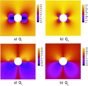
Figure 1: $Q_{2}$ and $Q_{3}$ for (a) $\lambda_{e}/R=10$ and (b) $5$ at $\varepsilon_{1}/\varepsilon_{0}=1$ in the range $-100\leq x\leq 100$ and $-100\leq z\leq 100$ in units of $\xi/2$ (see Eq.(3.2)). The $z$ axis is vertical and the $x$ axis is horizontal. There is a Saturn-ring defect in (a) and no defect in (b).

IV.2 Orientation for $\varepsilon_{1}>0$

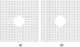
Figure 2: Nematic director $n$ in the $xz$ plane for (a) $\lambda_{e}/R=10$ and (b) $5$ at $\varepsilon_{1}/\varepsilon_{0}=1$. A Saturn ring is present in (a) and is nonexistent in (b).

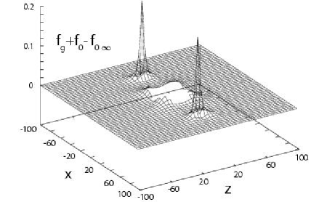
Figure 3: Landau-de Gennes free energy density $f_{g}+f_{0}-f_{0\infty}$ for $\lambda_{e}/R=10$ and $\varepsilon_{1}/\varepsilon_{0}=1$ in the $xz$ plane, where $f_{0\infty}$ is the background value of $f_{0}$. It is peaked at the Saturn ring.

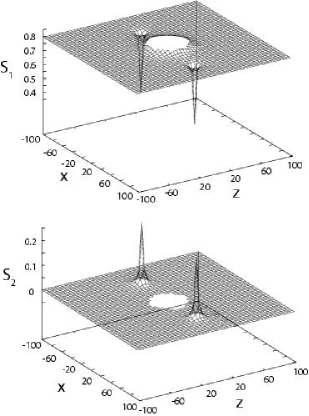
Figure 4: Scalar order parameter $S_{1}$ and biaxiality parameter $S_{2}$ for $\lambda_{e}/R=10$ and $\varepsilon_{1}/\varepsilon_{0}=1$ in the $xz$ plane.

We first focus on the case $\varepsilon_{1}/\varepsilon_{0}=1$, where the parallel alignment $\mbox{\boldmath$n$}\parallel{\mbox{\boldmath$E$}}$ is favored near the particle. This corresponds to the homeotropic alignment (perpendicular to the surface) in the neutral case. In Fig.1, we display $Q_{2}$ and $Q_{3}$ in Eq.(2.27) in the $xz$ plane for (a) $\lambda_{e}/R=5$ and (b) $10$. These quantities are related to $n$ as in Eqs.(2.32) and (2.33). Figure 2 displays the corresponding configuration of ${\mbox{\boldmath$n$}}=n_{\rho}{\mbox{\boldmath$e$}}_{\rho}+n_{z}{\mbox{\boldmath$e$}}_{z}$ in the $xz$ plane deduced from Eq.(2.31). For large $\lambda_{e}/R$, the nematic exhibits a radial orientation at the surface of the particle and a line of $-1/2$ defect appears surrounding the particle in the plane $z=0$, because the orientation is along the $z$ axis far from the particle. Such a circular defect line is called ”Saturn ring” in the literature Lav00 ; Ter95 ; Lub98 . In Fig. 2, we can see a -1/2 defect on both sides of the particle on the $x$ axis for $\lambda_{e}/R=10$ in (a), but there is no defect for $\lambda_{e}/R=5$ in (b).

In Fig.3, we plot the deviation of the Landau-de Gennes free energy density $f_{g}+f_{0}-f_{0\infty}$ at $\lambda_{e}/R=10$, where $F_{0}=\int d{\mbox{\boldmath$r$}}f_{0}$ and $F_{g}=\int d{\mbox{\boldmath$r$}}f_{g}$ are given in Eqs.(2.3) and (2.4). The $f_{0\infty}$ is the value of $f_{0}$ far from the particle in the uniaxial state with $S_{1}=S_{b}$ and $S_{2}=0$ (see Eq.(4.1)). This figure clearly demonstrates the existence of a Saturn ring at the sharp peaks. Next, in Fig.4, we display $S_{1}$ in Eq.(2.29) and $S_{2}$ in Eq.(2.30), respectively, for $\lambda_{e}/R=10$. At the defect positions, $S_{1}$ becomes small and $S_{2}$ exhibits a peak, while they tend to their bulk values, $S_{1}=0.79$ and $S_{2}=0$, far from the defect. In the defect region, the nematic is locally melt and biaxial. The latter biaxial behavior was also found in the previous molecular dynamics simulation for a neutral particle under the homeotropic anchoring Lav00 ; Allen .

We performed simulations for various other parameters (not shown here). With increasing $\lambda_{e}/R$, a Saturn ring appears suddenly with a nonvanishing radius at a certain transition value of $\lambda_{e}/R$ (see Fig.9 below). Essentially the same behavior can be observed with increasing $\varepsilon_{1}/\varepsilon_{0}$ at fixed $\lambda_{e}/R$. At small $\lambda_{e}/R$, the coupling between the electric field and the nematic order is not strong enough to induce the radial orientation on the equatorial plane. We therefore observe the quadrupolar symmetry without defect formation for $\lambda_{e}/R=5$ in Figs.1 and 2, where $S_{1}$, $S_{2}$ and $f_{0}+f_{g}$ exhibit no peaks around the particle.

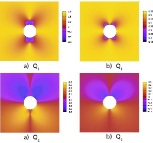
Figure 5: $Q_{2}$ and $Q_{3}$ for (a) $\lambda_{e}/R=10$ and (b) $4.2$ at $\varepsilon_{1}/\varepsilon_{0}=-1$ in the $xz$ plane.

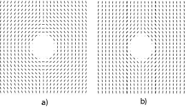
Figure 6: Nematic director $n$ for (a) $\lambda_{e}/R=10$ and (b) $4.2$ at $\varepsilon_{1}/\varepsilon_{0}=-1$ in the $xz$ plane. A pair of point defects can be seen in (a), while there is no defect in (b).

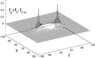
Figure 7: Landau-de Gennes free energy density $f_{0}+f_{g}-f_{0\infty}$ for $\lambda_{e}/R=10$ and $\varepsilon_{1}/\varepsilon_{0}=-1$ in the $xz$ plane, where $f_{0\infty}$ is the background value of $f_{0}$. It is peaked along the disclination line segments connecting the poles and the point defects.

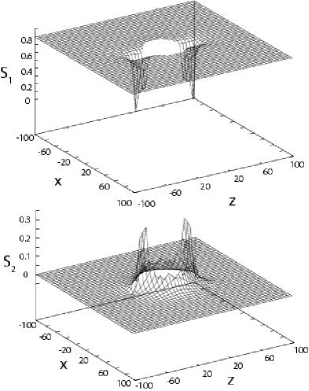
Figure 8: Scalar order parameter $S_{1}$ and biaxiality parameter $S_{2}$ for $\lambda_{e}/R=10$ and $\varepsilon_{1}/\varepsilon_{0}=-1$ in the $xz$ plane. They deviate from the background values around the disclination line segments.

IV.3 Orientation for $\varepsilon_{1}<0$

We turn to the second case $\varepsilon_{1}<0$ at $\varepsilon_{1}/\varepsilon_{0}=-1$, where the perpendicular alignment $\mbox{\boldmath$n$}\perp{\mbox{\boldmath$E$}}$ is preferred close to the particle. We show $Q_{2}$ and $Q_{3}$ in Fig.5 and $n$ in Fig.6 for (a) $\lambda_{e}/R=10$ and (b) $4.2$ in the $xz$ plane. Remarkably, in (a) the director is everwhere parallel to the surface and a pair of point defects are created on the $z$ axis, while in (b) the director is not parallel to the surface in the neighborhood of the poles. With these defects in (a), the Landau-de Gennes free energy density $f_{0}+f_{g}$ exhibits twin maxima at the point-defects as in Fig.7, while $S_{1}$ and $S_{2}$ behave as in Fig.8.

The defect structure in (a) has never been reported in the literature. Each point defect is detached from the surface and is connected to one of the poles by a $+1$ disclination line segment with length $\ell_{d}$. Here $\ell_{d}=37$ in (a). In fact, on both sides, a ridge structure with its top at the point-defect can be seen in $f_{0}+f_{g}$, $S_{1}$, and $S_{2}$ in Figs. 8 and 9. The singular line segments created are specified by $R<|z|<R+\ell_{d}$ and $\rho=0$, on which our numerical analysis yields $Q_{3}=0$ and $Q_{1}=-Q_{2}/2>0$, so that

$${\tensor{Q}}=Q_{1}({\tensor{I}}-3{\mbox{\boldmath$e$}}_{z}{\mbox{\boldmath$e$}}_{z}).$$ (4.9)

Here ${\tensor{I}}$ is the unit tensor. This form is natural from the rotational invariance around the $z$ axis and $n_{z}=0$. On these line segments, the equality,

$$S_{1}=S_{2}=3Q_{1}/2,$$ (4.10)

can be found from Eqs.(2.29) and (2.30). To see the defect structure in more dtail, we plot $S_{1}$ and $S_{2}$ as functions of $z$ for $\rho=0$ (along the $z$ axis) and $\rho=3$ in Fig.9 and $S_{1}$, $S_{2}$, and $n_{z}$ as functions of $\rho$ for $z=30$ in Fig.10. We can see how $S_{1}$ becomes small and equal to $S_{2}$ along the $z$ axis, while $S_{1}>S_{2}$ not on the $z$ axis. We also recognize that $n_{z}$ changes slowly on the scale of $R$, while $S_{1}$ and $S_{2}$ change on the scale of the core radius. A high degree of biaxiality is present around the line segments. In particular, $S_{1}=S_{2}$ on the singular line segments and $S_{1}>S_{2}$ outside them.

In the neutral case with short-range anchoring, a pair of point defects, called boojums P1 ; Volovik , are attached to the surface at the poles for large negative $W_{a}$.

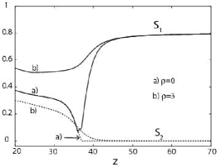
Figure 9: $S_{1}$ (solid line) and $S_{2}$ (dotted line) along the $z$ axis with $\lambda_{e}/R=10$ and $\varepsilon_{1}/\varepsilon_{0}=-1$ for (a) $\rho=0$ and (b) $\rho=3$, where $S_{1}=S_{2}$ on the line segment $R<z<R+\ell_{d}$ at $\rho=0$.

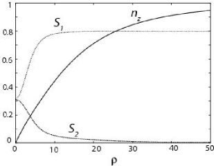
Figure 10: $S_{1}$ (dotted line), $S_{2}$ (dotted line), and $n_{z}$ (solid line) at $z=30$ along the $\rho$ axis for $\lambda_{e}/R=10$ and $\varepsilon_{1}/\varepsilon_{0}=-1$.

IV.4 Defect - no defect transition

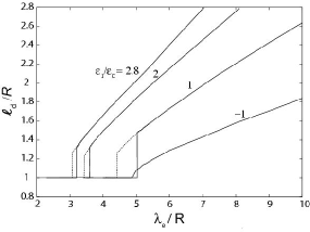
Figure 11: Normalized defect radius $\ell_{d}/R$ vs $\lambda_{e}/R$ for various $\varepsilon_{1}/\varepsilon_{0}$. For positive $\varepsilon_{1}$ the defect formation and collapse are discontinuous, where the solid and dotted curves are the results of increasing and decreasing $\lambda_{e}$, respectively. For negative $\varepsilon_{1}$ the transition is continuous with a critical point.

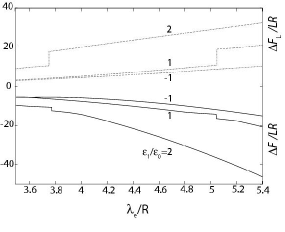
Figure 12: Normalized changes of the total free energy Eq.(4.7) (solid lines) and the Landau-de Gennes free energy Eq.(4.6) (broken lines) vs $\lambda_{e}/R$ for three $\varepsilon_{1}/\varepsilon_{0}$. For $\varepsilon_{1}>0$ the discontinuities correspond to the defect formation in Fig.11.

To gain quantitative information, we computed the distance of the defect core from the particle center $\ell_{d}$ as a function of $\lambda_{e}/R$ for various values of $\varepsilon_{1}/\varepsilon_{0}$. As shown in Fig.11, a Saturn ring appears discontinuously for positive $\varepsilon_{1}$. The solid curves were obtained when $\lambda_{e}$ was increased from small values, while the dotted curves were obtained when $\lambda_{e}$ was decreased from large values. We can see that the value of $\lambda_{e}/R$ at the formation is larger than that at the disappearance. Similar hysteresis behavior was also found in a two-dimensional simulation with positive $W_{a}$ by YamamotoYama . For negative $\varepsilon_{1}$, a pair of defects appear from the surface continuously and is detached for $\lambda_{e}/R$ larger than the critical value ($\sim 4.9$ in Fig.11). For both positive and negative $\varepsilon_{1}$, the transition value of $\lambda_{e}/R$ decreases with increasing $|\varepsilon_{1}|/\varepsilon_{0}$ (not shown for negative $\varepsilon_{1}$). These transitions are consistent with the criterion (3.7) since the defect formation is possible only in the strong solvation condition. Furthermore, once the defect is created, the defect size $\ell_{d}$ grows linearly with $\lambda_{e}/R$, with the slope increasing with increasing $|\varepsilon_{1}|/\varepsilon_{0}$ (which is the case also for negative $\varepsilon_{1}$). This trend is also consistent with Eq.(3.7), provided that the distance of the orientation deformation $\ell$ there and the defect size $\ell_{d}$ here are assumed to be of the same order.

Next, in Fig. 12, we plot the increase of the Landau-de Gennes free energy,

$$\Delta F_{\rm L}=\int_{r>R}d{\mbox{\boldmath$r$}}[f_{0}+f_{g}-f_{0\infty}],$$ (4.11)

and that of the total free energy,

$$\Delta F=F-F_{\rm un}=\Delta F_{L}+\Delta F_{e},$$ (4.12)

as a function of $\lambda_{e}/R$ for three values of $\varepsilon_{1}/\varepsilon_{0}$, where $\Delta F_{e}$ is the increase of the electrostatic part. These quantities were calculated outside the particle $r>R$ using the solutions of Eq.(2.39) and Eqs.(2.41)-(2.43). The $F_{\rm un}$ is the value of $F$ in the unperturbed state in which the orientation is uniaxially along the $z$ axis and the electric potential $\phi$ is calculated using the homogeneous $\varepsilon_{ij}$ in the uniaxial state. Thus these increases vanish as $\lambda_{e}/R\rightarrow 0$. We recognize that $\Delta F_{\rm L}$ increases but $\Delta F$ decreases with increasing $\lambda_{e}/R$. These aspects are consistent with the estimations in Eqs.(3.4) and (3.8), though they are rough approximations. It is remarkable that $\Delta F_{e}$ is negative and its absolute value is larger than $\Delta F_{\rm L}$. In addition, at the Saturn-ring formation, $\Delta F/LR$ changes by $-1.1$ and $-0.9$ for $\varepsilon_{1}/\varepsilon_{0}=1$ and 2, respectively, while the corresponding changes of $\Delta F_{\rm L}/LR$ are 8.2 and 7.1, respectively. Notice also that $\Delta F_{\rm L}$ and $\Delta F$ are continuous even at the defect formation for negative $\varepsilon_{1}$.

V Summary and discussions

We summarize our main results. In Sec.2, we have derived the equilibrium equations for the tensor order parameter $Q_{ij}$ as in Eq.(2.16), supplemented with the Poisson equation (2.12). The interaction between the orientation and the electric field arises from the dielectric anisotropy $\varepsilon_{1}$ in Eq.(2.13). In the axisymmetric case $Q_{ij}$ is expressed in terms of the three components $Q_{i}$ ($i=1,2,3$) as in Eq.(2.27). They are determined by Eqs.(2.41)-(2.43) with the aid of the Poisson equation Eq.(2.39). In Sec.3, we have estimated the range $\ell$ of the strong orientation deformation around an isolated charged particle as in Eq.(3.5) and obtained the criterion of the strong deformation as in Eq.(3.7). There, we can see analogy between the present problem of liquid crystals and that of the ion solvation in polar fluids Kit04 . For a highly charged colloidal particle, we have found the effective anchoring parameter Eq.(3.12) under the condition Eq.(3.9). In Sec.4, we have numerically examined the orientation deformation around an isolated charged particle. For positive $\varepsilon_{1}$ and for large $\lambda_{e}/R\propto Z/R$, we have obtained a Saturn ring around the particle, where $\lambda_{e}$ is the characteristic length in Eq.(3.6). As shown in Fig.11, the defect radius exhibits a discontinuous change as a function of $\lambda_{e}/R$ for positive $\varepsilon_{1}$. This means that a Saturn ring appears or disappears suddenly with radius larger than $R$ as $\lambda_{e}/R$ is increased or decreased. For negative $\varepsilon_{1}$ and large $\lambda_{e}/R$, we have found appearance of point defects (boojums) on both sides of the particle along the $z$ axis as a continous transition. They are detached from the surface, while they are on the surface for a neutral particle. As shown in Fig.12, the decrease of the electrostatic free energy overcomes the increase of the Landau-de Gennes free energy, resulting in the lowering of the total free energy, with the orientation deformation.

We make further comments on the limitations of our work and future problems.
(i) In our simulations we have sought only the axisymmetric defrmations symmetric with respect to the $xy$ plane. However, as in the neutral case Lav00 ; Ter95 ; Lub98 ; P1 , there can be symmetry-breaking defects such as a combination of a radial and a hyperbolic hedgedog.
(ii) The orientation deformation occurs much longer than the particle radius. For microscopic ions the deformation extends over a nanometer scale. From Fig.12 we can see that the lowering of the free energy much exceeds $LR\sim k_{B}TR/a$, where $a$ is the size of a liquid crystal molecule. Thus, even for $R\sim a$, we find $|\Delta F|\gg k_{B}T$ and the deformation can be stable against thermal fluctuations. As mentioned in Sec.1, the long-range deformation should be the origin of anomalously low ion mobility in nematics Gen93 ; PG . However, the existence of defects on a nanometer scale is not well established because of the limitation of our coarse-grained approach.
(iii) We have examined the charge effect only in nematics. Slightly above the (weakly first-order) isotropic-nematic phase transition, the deformation around charged particles can be long-ranged, extending over the correlation length Fukuda , as in near-critical polar fluids Kit04 . Furthermore, metastability or hysteresis behavior at the isotropic-nematic transition should almost disappear in the presence of a small amount of ions, owing to ion-induced nucleation, as in polar fluids Kit05 .
(iv) We have presented numerical analysis only for a single particle, but long-range correlations among charged inclusions can produce a number of unexplored effects. In particular, doping of a small amount of ions into liquid crystals should provide highly correlated ionic systems, where transparent nematic states would be realized Yam01 . Ion solubility and ion distribution across an isotropic-nematic interface should constitute new problems, which have been studied for polar fluids Onuki2006 .
(v) We should investigate dynamical properties of charged particles in liquid crystals such as the ion mobility or convection Gen93 ; Fukuda . They should be much influenced by the orientation deformation omoto .
(vi) Beyond the particular interest in the field of liquid crystals, the general approach developed in this paper and preceding ones Kit04 ; Kit05 ; NATO ; Onu04 ; Onuki2006 using inhomogeneous dielectric constant or tensor could provide a practical and coherent method to study various polarization effects in simple and complex fluids.

- (1) P. Poulin, H. Stark, T.C. Lubensky and D.A. Weitz, Science 275, 1770 (1997).
- (2) M. Zapotocky, L. Ramos, P. Poulin, T.C. Lubensky, and D.A. Weitz, Science283, 209 (1999).
- (3) O.D Lavrentovich, P. Pasini, C. Zannoni, and S. Zumer (Editors), Defects in Liquid Crystals: Computer Simulation, Theory and Experiment, NATO Science Series II: 43 (Kluwer Academic, Dordrecht, 2001).
- (4) E.M. Terentjev, Phys. Rev. E 51, 1330 (1995).
- (5) T.C. Lubensky, D. Pettey, N. Currier, and H. Stark, Phys. Rev. E 57, 610 (1998).
- (6) P. Poulin and D. Weitz, Phys. Rev. E 57, 626 (1998).
- (7) D. Andrienko, G. Germano, and M. P. Allen, Phys. Rev. E 63, 041701 (2001).
- (8) R. Yamamoto, Phys. Rev. Lett. 87, 075502 (2001).
- (9) S.P. Meeker, W.C.K. Poon, J. Crain, and E.M. Terentjev, Phys. Rev. E 61, R6083 (2000).
- (10) J. Yamamoto and H. Tanaka, Nature 409, 321 (2001).
- (11) T. Bellini, M. Caggioni, N. A. Clark, F. Mantegazza, A. Maritan, and A. Pelizzola, Phys. Rev. Lett. 91, 85704 (2003).
- (12) J.-i. Fukuda, H. Stark and H. Yokoyama, Phys. Rev. E 69, 021714 (2004).
- (13) H. Stark, J.-i. Fukuda, and H. Yokoyama, J. Phys.: condensed matter 16, S1957 (2004).
- (14) In the neutral case, the dimensionless anchoring strength is given by , where is the Frank coefficient in Eq.(2.22). Defects are formed for .
- (15) A. Onuki, in Nonlinear Dielectric Phenomena in Complex Liquids, NATO Science Series II: 157, edited by S.J. Rzoska (Kluwer Academic, Dordrecht, 2004).
- (16) A. Onuki, J. Phys. Soc. Jpn. 73, 511 (2004).
- (17) P.G. de Gennes and J. Prost, The Physics of Liquid Crystals (Clarendon, Oxford, 1993).
- (18) P.G. de Gennes, Comments Solid State Phys. 3, 148 (1971).
- (19) M. Born, Z. Phys. 1, 45 (1920).
- (20) J. N. Israelachvili, Intermolecular and Surface Forces (Academic Press, London, 1991).
- (21) A. Onuki and H. Kitamura, J. Chem. Phys 121, 3143 (2004). In addition to the microscopic solvation shell, long-range density (or composition) deviations are induced around an ion in near-critical polar fluids.
- (22) N. Schopohl and T. J. Sluckin, Phys. Rev. Lett. 59, 2582 (1987)
- (23) A. Sonnet, A. Kilian, and S. Hess, Phys. Rev. E 52, 718 (1995).
- (24) J. C. Loudet and P. Poulin, Phys. Rev. Lett. 87, 165503 (2001).
- (25) In the vicinity of small charged particles, the electric field can be very strong and the effect of nonlinear dielectric saturation needs to be considered.
- (26) W. Pyzuk, I. Stomka, J. Chrapeć, S.J. Rzoska, and J. Zioło, Chem Phys. 121, 255 (1988). In this experiment the nonlinear dielectric behavior was observed above the transition under homogeneous electric field .
- (27) Let us set in the region . Then the space integration of the Franck free energy density in Eq.(2.22) in this region becomes .
- (28) A.G. Moreira and R.R. Netz, Phys. Rev. Lett. 87, 078301 (2001); Eur. Phys. J. E 8 33 (2002).
- (29) G.E. Volovik and O.D Lavrentovich, Sov. Phys. JETP 58, 1159 (1983).
- (30) J.-i. Fukuda, H. Stark, and H. Yokoyama Phys. Rev. E 72, 021701 (2005).
- (31) H. Kitamura and A. Onuki, J. Chem. Phys. 123, 124513 (2005).
- (32) A. Onuki, Phys. Rev. E, 73, 021506 (2006).
- (33) T. Omoto, Master thesis (2005), Department of Physics, Kyoto University, Japan.