Density matrix renormalization group algorithms for Y-junctions

Abstract

Systems of Y-junctions are interesting both from a fundamental viewpoint and because of their potential use in nanoscale devices. These systems can be studied numerically with the density matrix renormalization group(DMRG), but existing algorithms are inefficient. Here, we introduce a much more efficient DMRG algorithm for Y-junction systems. As an example of the use of this method, we study $S=\frac{1}{2}$ bound states in Heisenberg $S=1$ junctions with two geometries, one where the junction consists of a single site, and the other where it consists of a triangle of three sites.

Junctions are essential ingredients of existing and future electronic and spintronic devices. As progress towards smaller and smaller devices continues, eventually we will reach the atomic scale. Perhaps the smallest conceivable junctions are composed of intersecting spin or electron chains, with each site representing a single atom. Isolated chains, modeled by Heisenberg, Hubbard, and related Hamiltonians, have been extensively studied. Yet surprisingly little work has been done on the corresponding junctions of three or more half-chains, or legs. There has been recent work on junctions of quantum wires. For example, Oshikawa, et alCOA03 ; OCA06 studied the transport properties of a junction composed of three quantum wires enclosing a magnetic flux, modeling the chains as spinless Tomonaga-Luttinger liquids, and finding a rich phase diagram. Quantum Monte Carlo on junctions of fermion chains are subject to the minus sign problem, so little numerical work has been done. We are not aware of any studies which have focused on junctions of spin chains.

Our present work has two main aspects. First, we develop a new density matrix renormalization group (DMRG) algorithm for studying junctions. Ordinary DMRGdmrg is much less efficient for junctions compared to chains with open boundaries; our new method requires only slightly more computational effort. Second, as an application of this method we consider a key feature of a few of the simplest junctions, namely the presence of $S=\frac{1}{2}$ “spinon” bound states in two types of $S=1$ Heisenberg Y junctions. These bound states are the analogues of the spin-$\frac{1}{2}$ end states found in open $S=1$ chainsWH93 ; GGLKM91 . They exist at any $S=1$ junction with an odd number of legs, regardless of the local interactions at the junction. Magnons coming to the junction can interact with the bound state via spin-flip scattering, leading to potentially interesting dynamical phenomena. We call these spinon bound states because a spin-$\frac{1}{2}$ degree of freedom is bound to the junction, but it is important to note that they are features of the ground state. A separate issue, which we do not address here, is whether the lowest excited state is below the Haldane gap, representing, say, a magnon bound to the junction. For example, a single $S=\frac{1}{2}$ impurity in a $S=1$ chain has such a bound state below the gap only for sufficiently weak coupling to the impuritysorensen .

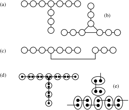
Figure 1: Schematic view for the geometric configuration and algorithm for Y-junctions.The geometry of the Y-junctionis shown in (a), where the circles represent sites and the solid lines represent connections. The alternative geometry Y_Δ junction is shown in (b). The original DMRG method is shown in (c), where one cuts the link between two sites and relinks it to the center of the remaining chain, making it topologically equivalent to a Y-junction. Verstraete and Cirac’s tensor representation is shown in (d), where each open circle represents a tensor and each solid dot represents a tensor index. An Affleck-Kenedey-Lieb-Tasaki valence bond picture of the Y-junction is shown in (e), where each solid dot represents a $S=\frac{1}{2}$, the line segments represent valence bonds, and where each open circle represents a projection operator to the $S=1$ subspace for a site.

We consider two types of three-leg junctions, which we will label Y and Y_Δ, where we think of the $\Delta$ as a triangle. These are shown in Fig. 1(a) and (b). DMRG is extremely efficient for one dimensional systems with short range interactions. It is standard to treat two-dimensional strips by mapping the strip into a chain with interactions over a distance of several lattice spacings. Similarly, a Y junction can be treated as a chain with one long range interaction, shown in Fig. 1(c). The long-range interaction is equivalent to periodic boundary conditions in terms of the effort necessary in DMRG: a typical block of sites connects to the rest of the system by two links in both cases. If $m$ states per block are required for a given accuracy for a single chain, one expects roughly $m^{2}$ states to be needed for the Y junction (or a periodic chain). This changes the computational effort from $O(Nm^{3})$ to $O(Nm^{6})$, where $N$ is the number of sites.

As discussed below, our new algorithm scales as $O(Nm^{3}+m^{4})$. Typically $m$ and $N$ are similar in size (say $\sim 10^{2}$), so the cost is close to that of a single chain, and a large improvement over the method with a long-range interaction. Our algorithm is somewhat related to Otsuka’s early DMRG treatment of the XXZ model on a Bethe latticeOtsuka . It is closely related to Shi, Duan, and Vidal’s very recent treatmentTree of general tree-tensor networks using Vidal’s time-evolving block decimation method, which is closely related to DMRG. One can also view it as perhaps the simplest step towards an implementation of Verstraete and Cirac’s much more complicated tensor approachmps ; PEPS , which holds great promise for true two dimensional systems.

Consider the matrix product representation for the wavefunction in standard DMRGOR95

$$|\Psi\rangle=A[s_{1}]A[s_{2}]A[s_{3}]...A[s_{n}]|s_{1}s_{2}s_{3}...s_{n}\rangle$$ (1)

where $s_{i}$ labels the states of site $i$, and $A[s_{i}]$ is a matrix except for the first and last sites, where it is a vector. One can view each matrix as a two-dimensional tensor, with indices connecting to the left and right. In Verstraete and Cirac’s approach for a square lattice, one generalizes to four-dimensional tensors, with indices connecting to each nearest neighbor. In our approach, only one tensor is needed, at the junction site, and it has only three indices. All sites on the legs are ordinary matrices, as shown in Fig. 1(d). Unlike in the more general tensor approach, the states can be easily described in terms of an orthogonal basis.

Figure 2: Configurations illustrating the new DMRG algorithm. The procedure starts from the center (a), where two legs are combined to form a new system block. The sweep next progress down a single leg, as in (b), reaches the end of the leg, (c), and comes back to the center.

The key to our approach is a new type of step for the junction. In this “junction step” the system is divided into three blocks instead of two (one for each leg), and the calculation time is higher, $O(m^{4})$, where $m$ is the number of states kept per block, instead of $O(m^{3})$. The rest of a sweep consists of steps involving two blocks, where one of the blocks contains two legs plus part of the third. The sweep moves out to the end of one leg, and then back to the center, after which the junction step is repeated, and then the sweep goes out another leg, etc., until all legs have been treated.

We now describe this method in more detail. The system is built up in a warmup sweep. An ordinary DMRG chain initialization sweep is first carried out on one leg of the Y-junction. For the environment block one can use the next several sites of the leg, or artifically reflect the leg–the algorithm is not very sensitive to the warmup, and we keep only a small number of states $m$, storing the related operator matrices and transformation matrices. One continues until the entire leg is incorporated into the block. At the last few steps the environment may or may not be in the form of a junction—it does not make much difference. This block is then duplicated twice to form the other two legs.

At this point, the finite-system sweeps begin. The first step is the junction step. For the Y-junction, where the junction consists of a single site, that site is incorporated into one leg. The wavefunction can be written as $\psi_{ijk}$, where $i$, $j$, and $k$ refer to the three legs/blocks. Applying the operators appearing in the Hamiltonian $H$ to $\psi$ requires a calculation time of $O(m)^{4}$, in contrast to the $O(m)^{3}$ time on a chain. For example, to apply the term $S_{ii^{\prime}}^{z}S_{jj^{\prime}}^{z}$ connecting the first two legs, one first multiplies the matrix $S_{jj^{\prime}}^{z}$ into $\psi_{i^{\prime}j^{\prime}k}$, storing the result, and then multiplies that result by $S_{ii^{\prime}}^{z}$. Several such multiplications by $H$ are performed to make a few Lanczos or Davidson steps to find an approximate ground state $\psi$.

After finding $\psi$ we want to combine two legs (say $j$ and $k$) into a single effective block, as shown in Fig. 2(a). In ordinary DMRG, we find the reduced density matrix for the system block, and diagonalize it, which in this case would result in a calculation time of $O(m^{6})$. Instead, we perform a singular value decomposition (SVD) on $\psi$, treating $j$ and $k$ together as a single combined index, and $i$ as the other index of the matrix. The SVD has a calculation time of only $O(m^{4})$, but is equivalent to the density matrix diagonalization. (Note, however, that the SVD is not as easily generalized to having more than one state targeted.) One obtains transformation matrices $O_{\alpha,jk}$, where $\alpha$ are the new states of the combine blocks. The operators for the combined block $A^{\prime}$ are obtained as $OAO^{T}$; this can also be performed in $O(m^{4})$ time. For example, to transform $S^{+}_{jj^{\prime}}S^{-}_{kk^{\prime}}$, one first forms $X_{\alpha,j^{\prime}k}=O_{\alpha,jk}S^{+}_{jj^{\prime}}$, then $Y_{\alpha^{\prime},j^{\prime}k}=S^{-}_{kk^{\prime}}O_{\alpha^{\prime},j^{\prime}k^{\prime}}$, and then contracts $XY$ over indices $j^{\prime}k$.

Next, as shown in Fig. 2(b), we sweep down leg $i$. This sweep is an ordinary DMRG sweep, with calculation time $O(m^{3})$ per site; the fact that the system block now includes two legs does not affect calculations in each step. We continue moving to the edge of the leg, Fig. 2(c), and then turn around and come back to the center. The junction step is performed and then the sweep moves out one of the other legs. The three legs need not be identical; the sweep treats each independently. In each full sweep, the center step is performed three times. Alternatively, if the Hamiltonian and the desired state are symmetric with respect to the interchange of legs, just before the junction step one can replace each of the legs with the most recently updated leg/block.

Figure 3: Error in the energy as a function of the number of states kept $m$ for the new and the standard DMRG algorithms. The reference energy $E$ here is the result of standard algorithm by keeping $3000$ states.

For an $3\times N$ system, the total cpu time is $O(m^{4}+Nm^{3})$. In comparison, we consider the standard DMRG calculation with one long range interaction. In Fig. 3 we show the error in the energy as a function of the number of states kept for the new versus the standard algorithm; the new algorithm requires vastly fewer states. If we assume the long range interaction mandates $O(m^{2})$ states be kept for sufficient accuracy (for large $N$), the standard DMRG calculation would scale as $O(Nm^{6})$.

We now use the new algorithm to study $S=\frac{1}{2}$ bound states in $S=1$ Heisenberg junctions. A simple consideration of quantum numbers makes the presence of the bound states clear. An $S=1$ open chain has $S=\frac{1}{2}$ states on the ends, and a finite correlation length $\xi=6.03$WH93 . The ends of the legs in a large junction system will also have $S=\frac{1}{2}$ states; the finite correlation length does not allow the junction to influence the ends. With an odd number of legs, a half-integer-spin state must form at the junction to make the total spin an integer. For a junction formed from very weakly coupled legs, the bound state comes from coupling three effective $S=\frac{1}{2}$ states at the junction. For more strongly coupled legs one can think in terms of the Affleck-Kennedy-Lieb-Tasaki (AKLT) pictureAKLT where each $S=1$ is composed of two $S=\frac{1}{2}$’s, with one valence bond singlet connecting two $S=\frac{1}{2}$’s on each near-neighbor link; see Fig. 1(e). At the junction, there must be one $S=\frac{1}{2}$ left over after the singlets are formed.

Figure 4: Results for $\langle Sz(l)\rangle$ for a Y-junction as a function of site $l$ along a chain, compared with an open 1D chain. For the Y-junction, the first site shown is the center junction site. Here, the total spin of the system is $S_{z}=\frac{1}{2}$.

In order to study the junction bound state, it is convenient to place a real $S=\frac{1}{2}$ spin on the end of each chain (far from the junction), which forms a singlet with the effective $S=\frac{1}{2}$, eliminating it as a low energy degree of freedom. For the Y-junction, the ground state is then a nondegenerate doublet corresponding to total $S_{z}=\pm\frac{1}{2}$. In Fig. 4 we show $\langle S_{z}(l)\rangle$ as a function of site $l$ for a $3\times 60$ Y-junction. The result for the other two legs is identical. We see a strong similarity with the results for the end state of a single chain, except for a smaller magnitude of the oscillations. The decay of the oscillations is consistent with an exponential decay with the correlation length of a single chainWH93 . Looking near the junction we find the initially surprising result that the value of $|\langle S_{z}\rangle|$ at the junction site (0.30) is less than that on the first site of a leg (0.34). If one thinks in terms of a mean-field/classical picture, with the spin fluctuations acting like thermal fluctuations, one would expect the opposite: the junction site is surrounded by three polarized spins, and would experience a larger polarizing field than the adjacent sites which have only two neighbors. However, if one utilizes the AKLT valence bond picture instead, one would predict a smaller magnitude at the junction site: the extra unpaired $S=\frac{1}{2}$ is energetically favored to be on an adjacent site, with one missing valence bond, as shown in Fig. 1(e). An unpaired spin on the junction site occurs from fluctuations of the unpaired $S=\frac{1}{2}$ from leg to leg.

Figure 5: Results for $\langle Sz(l)\rangle$ for a $3\times 60$ Y_Δ-junction, where site 0 is part of the junction triangle.

Now consider the other geometric configuration, the Y_Δ-junction. Fig. 5 shows $\langle S_{z}(l)\rangle$ for a Y_Δ-junctionwith size $3\times 60$. One sees the presence of a bound state at the junction, as for the Y-junction. However, the symmetry under interchange of legs is broken by an exact ground state degeneracy.

To understand this degeneracy, consider a three-site $S=\frac{1}{2}$ Heisenberg triangle. The $S=\frac{1}{2}$ triangle is clearly relevant in the limit that the exchange couplings connecting the three junction sites to each other is very small. In that case the $S=\frac{1}{2}$’s are the end states of each leg. In the opposite limit, where the exchange between the $S=1$’s in the junction is large, the ground state of the $S=1$ triangle is nondegenerate (with a gap of precisely $J$), but then one expects a $S=\frac{1}{2}$ end state on each leg starting at the site adjacent to the junction, and one would expect these three $S=\frac{1}{2}$’s to be weakly coupled antiferromagnetically through the central triangle.

If we square the total spin operator for a generic Heisenberg triangle, we obtain

$$\frac{E}{J}=\frac{1}{2}(S_{\rm tot}(S_{\rm tot}+1)-S_{1}(S_{1}+1)-S_{2}(S_{2}+1)-S_{3}(S_{3}+1)).$$ (2)

Here $S_{1}=S_{2}=S_{3}=\frac{1}{2}$, and $S_{\rm tot}$ can be either $\frac{1}{2}$ or $\frac{3}{2}$. The ground states have energy $-\frac{3}{4}J$ and consist of two degenerate $S_{\rm tot}=\frac{1}{2}$ doublets. If one regards the triangle as a periodic chain, then the degeneracy corresponds to total momenta around the triangle of $k=\pm 2\pi/3$. The $S_{\rm tot}=\frac{3}{2}$ multiplet has $k=0$ and energy $\frac{3}{4}J$. The Y_Δ-junction has the same degeneracy as the ground states of the triangle; the numerical calculation converges to a arbitrary linear combination of these states. We have confirmed the degeneracy behaves as expected by targetting several states on a relatively small Y_Δ-junction system.

In conclusion, we have presented a relatively simple DMRG algorithm for junction systems, with greatly improved computational effort. We have used this to study the $S=\frac{1}{2}$ bound states of two types of Heisenberg $S=1$ Y-junction.

We thank S. Chernyshev, F. Verstraete, and I. Affleck for helpful conversations. We acknowledge the support of the NSF under grant DMR03-11843.

References

- (1) C. Chamon, M. Oshikawa, and I. Affleck, Phys. Rev. Lett. 91, 206403(2003).
- (2) M. Oshikawa, C. Chamon, and I. Affleck, J. Stat. Mech(2006)P02008.
- (3) S.R. White, Phys. Rev. Lett. 69, 2863 (1992); Phys. Rev. B 48, 10345 (1993).
- (4) S.R. White, D.A. Huse, Phys. Rev. B48,3844(1993).
- (5) S.H. Glarum, S. Geschwind, K.M. Lee, M.L. Kaplan, and J. Michel, Phys. Rev. Lett. 67, 1614(1991).
- (6) Bound states (with ) have been found on the weak links of chains; see E. Sorensen and I. Affleck Phys. Rev. B51, 16115(1995).
- (7) H. Otsuka, Phys. Rev. B53, 14004(1996).
- (8) Y. Shi, L. Duan and G. Vidal, quant-ph/051107
- (9) F. Verstraete, D. Porras, and J.I. Cirac, Phys. Rev. Lett. 93, 227205 (2004).
- (10) F. Verstraete and J.I. Cirac, cond-mat/0407066
- (11) S. Ostlund and S. Rommer, Phys. Rev. Lett. 75, 3537(1995); S. Rommer and S. Ostlund, Phys. Rev. B55, 2164(1997).
- (12) I. Affleck, T.Kennedy, E.H. Lieb and H. Tasaki, Phys. Rev. Lett. 59, 799(1987).