Spin diffusion and the anisotropic spin-$1/2$ Heisenberg chain

Abstract

Measurements of the spin-lattice relaxation rate $1/T_{1}$ by nuclear magnetic resonance for the one-dimensional Heisenberg antiferromagnet Sr₂CuO₃ have provided evidence for a diffusion-like contribution at finite temperature and small wave-vector. By analyzing real-time data for the auto- and nearest-neighbor spin-spin correlation functions obtained by the density-matrix renormalization group I show that such a contribution indeed exists for temperatures $T>J$, where $J$ is the coupling constant, but that it becomes exponentially suppressed for $T\ll J$. I present evidence that the frequency-dependence of $1/T_{1}$ in the Heisenberg case is smoothly connected to that in the free fermion case where the exponential suppression of the diffusion-like contribution is easily understood.

I Introduction

Knowledge about the dynamical properties of the spin-$1/2$ Heisenberg chain $H=J\sum_{j}\boldsymbol{S}_{j}\boldsymbol{S}_{j+1}$, where $J>0$ is an antiferromagnetic coupling constant, is the link between theory and many experiments on compounds which are believed to be good realizations of this model. Whereas the static properties of the one-dimensional Heisenberg model are well understood based on effective low-energies theories and its Bethe Ansatz integrability, many open problems concerning the dynamical properties have only been addressed very recently. An important question, much interest has focused on, is how the integrability of the pure model as well as small integrability-breaking perturbations in any real material influence the spin (electrical) Zotos (1999); Rosch and Andrei (2000); Alvarez and Gros (2002); Fujimoto and Kawakami (2003); Benz et al. (2005) and heat conductivity.Klümper and Sakai (2002); Jung et al. (2006) A related question important for nuclear magnetic resonance (NMR), neutron scattering and Coulomb drag between quantum wires refers to the dynamic spin structure factor. A detailed analysis of its lineshape at zero temperature $T$ and small wave-vector $q$ has been presented recently in Refs. Pustilnik et al., 2003; Pereira et al., 2006; Pustilnik et al., 2006.

Experimentally, most efforts have been concentrated on the compound Sr₂CuO₃ which is believed to be an almost ideal realization of a one-dimensional spin-$1/2$ Heisenberg model with a large in-chain antiferromagnetic coupling constant $J\sim 2000$ K and very small inter-chain couplings leading to a Néel temperature $T_{N}\approx 5$ K $\sim 0.003\,J$. Its Heisenberg character is supported by measurements of the uniform susceptibility at low temperatures which are compatible with a logarithmic decrease expected due to marginally irrelevant Umklapp scattering.Eggert et al. (1994); Motoyama et al. (1996); Thurber et al. (2001) Measurements of the thermal conductivity have revealed strong spatial anisotropies and large parts of the heat current along the chain direction have been attributed to magnetic excitations.Sologubenko et al. (2001) In a pure Heisenberg model the heat current is a conserved quantity Zotos et al. (1997) leading to an infinite thermal conductivity $\kappa_{th}$.Klümper and Sakai (2002) The effect of small integrability-breaking perturbations has been investigated in Ref. Jung et al., 2006 and it has been found that $\kappa_{th}$ can remain anomalously large under certain circumstances. A possible explanation of the Sr₂CuO${}_{3}\,$conductivity data has been proposed in Ref. Rozhkov and Chernyshev, 2005 arguing that phonon and impurity mediated relaxation processes dominate. Another important test of the dynamical properties of this system at small frequencies $\omega$ has been provided by NMR measurements of the spin-lattice relaxation rate $1/T_{1}$. Particularly appealing is the possibility to separate the contributions from wave-vectors $q\sim 0$ and $q\sim\pi$, which are the dominant ones for low temperatures, by measuring $1/T_{1}$ at inequivalent lattice sites with different form factors.Takigawa et al. (1996); Thurber et al. (2001) Theoretical studies of the spin-lattice relaxation rate have so far been based on the calculation of the dynamical structure factor in the framework of low-energy effective theoriesSchulz (1986); Sachdev (1994) or the numerical calculation of imaginary-time correlation functions.Sandvik (1995); Starykh et al. (1997a); Takigawa et al. (1997); Naef et al. (1999) Recent progress in the calculation of real-time correlation functions by the density-matrix renormalization group (DMRG) both at zero temperatureWhite and Feiguin (2004) and finite temperatureSirker and Klümper (2005) has opened a new and so far unexplored avenue to tackle this problem.

In this article I will focus on the ¹⁷O NMR measurements in Sr₂CuO₃Thurber et al. (2001) where evidence for a $q\sim 0$ mode with diffusion-like character at finite temperature has been found. To test whether or not the spin-lattice relaxation rate behaves indeed qualitatively different in the Heisenberg than in the free fermion case, I will consider the $XXZ$-model which interpolates between these two cases. In Sec. II the basic theoretical framework to study spin-lattice relaxation will be layed out and predictions by the Luttinger model discussed. In Sec. III the free fermion case is considered in detail. The interacting case is then analyzed in Sec. IV based on real-time data for spin-spin correlation functions obtained by the DMRG method applied to transfer matrices.Sirker and Klümper (2005) In the last section I discuss and summarize my main conclusions.

II Basic theoretical framework

The Hamiltonian of the $XXZ$-chain is given by

$$H=J\sum_{j=1}^{N}\left[S_{j}^{x}S_{j+1}^{x}+S_{j}^{y}S_{j+1}^{y}+\Delta S_{j}^{z}S_{j+1}^{z}-hS^{z}_{j}\right]\;,$$ (1)

where $J>0$ is an antiferromagnetic coupling constant and $h$ the magnetic field. $\Delta$ parameterizes an exchange anisotropy and the model is critical for $-1<\Delta\leq 1$. By Jordan-Wigner transformation the model can be represented in terms of fermionic operators $\psi_{j}$

$$H = J\sum_{j=0}^{N}\left[\frac{1}{2}\left(\psi^{\dagger}_{j}\psi_{j+1}+\psi^{\dagger}_{j+1}\psi_{j}\right)-h\left(\psi^{\dagger}_{j}\psi_{j}-\frac{1}{2}\right)\right.$$ (2)

$$+ \left.\Delta\left(\psi^{\dagger}_{j}\psi_{j}-\frac{1}{2}\right)\left(\psi^{\dagger}_{j+1}\psi_{j+1}-\frac{1}{2}\right)\right]\;.$$

The fermions become non-interacting for $\Delta=0$. We assume for simplicity that the hyperfine interaction

$$H_{hf}=\sum_{r}A_{r}\boldsymbol{I}_{0}\boldsymbol{S}_{r}$$ (3)

between the nuclear spin $\boldsymbol{I}_{0}$ and the surrounding electron spins $\boldsymbol{S}_{r}$, where $r$ is the distance in units of the spacing between the electron spins, is isotropic. If the hyperfine interaction is the dominant relaxation process, the spin-lattice relaxation rate $1/T_{1}$ can be obtained by treating $H_{hf}$ as a perturbation inducing transitions between the nuclear levels leading toMoriya (1956)

$$\frac{1}{T_{1}}=\frac{1}{2}\sum_{r,r^{\prime}}A_{r}A_{r^{\prime}}\int_{-\infty}^{\infty}dt\,\text{e}^{i\omega_{N}t}\langle S_{r}^{+}(t)S_{r^{\prime}}^{-}(0)\rangle\;.$$ (4)

Here $\omega_{N}$ is the nuclear magnetic resonance frequency with $\omega_{N}\ll T$ in all NMR experiments. By Fourier transform we obtain

$$\frac{1}{T_{1}}=\frac{1}{2}\int\frac{dq}{2\pi}|A(q)|^{2}S^{+-}(q,\omega_{N})\;,$$ (5)

where the transverse dynamic spin structure factor is defined by

$$S^{+-}(q,\omega_{N}) = \sum_{j}\text{e}^{-\text{i}qj}S^{+-}_{j}(\omega_{N})$$ (6)

$$S^{+-}_{j}(\omega_{N}) = \int_{-\infty}^{\infty}dt\,\text{e}^{\text{i}\omega_{N}t}\langle S^{+}_{j}(t)S^{-}_{0}(0)\rangle$$

and

$$A(q)=\sum_{r}\text{e}^{iqr}A_{r}\;.$$ (7)

If the hyperfine interaction (3) is anisotropic, we have to replace $|A(q)|^{2}\to(|A_{x}(q)|^{2}+|A_{y}(q)|^{2})/2$ in Eq. (5). In spin-chain compounds there is usually no exchange anisotropy, i.e., $\Delta=1$. In this case we can replace the transverse by the longitudinal dynamic structure factor leading to

$$\frac{1}{T_{1}}=\int\frac{dq}{2\pi}|A(q)|^{2}S^{zz}(q,\omega_{N})\;.$$ (8)

Note, that the spin-spin correlation functions here in principle have to be evaluated for finite magnetic field. In experiments, however, we often have the situation that $T\gg|h|$ so that the effect of the magnetic field on the electron spins can be ignored.

In Sr₂CuO${}_{3}\,$, measurements of the spin-lattice relaxation rate have been performed on the copper sites,Takigawa et al. (1996) which carry the $S=1/2$ electron spin, as well as on the two inequivalent oxygen sites O(1) and O(2)Thurber et al. (2001) (see Fig. 1).

Figure 1: Schematic sketch of the spin chain Sr₂CuO${}_{3}\,$.

The hyperfine interaction drops down rapidly with distance. It is therefore reasonable to assume that only the on-site hyperfine interaction $A_{0}$ and nearest-neighbor hyperfine interaction $A_{1}$ are important leading to $A_{Cu}(q)=\int dq\exp(\text{i}qr)[A_{0}\delta(r)+A_{1}\delta(r\pm 1)]=A_{0}+2A_{1}\cos(q)$. For the O(2)-site, on the other hand, one finds

$$|A_{O(2)}(q)|^{2}=|A|^{2}$$ (9)

and for the O(1)-site

$$|A_{O(1)}(q)|^{2}=|B|^{2}\cos^{2}(q/2)\;,$$ (10)

where $A,B$ are material dependent constants. The spin-lattice relaxation rate at the O(2)-site can therefore be expressed as

$$1/T^{a}_{1}=|A|^{2}S^{zz}_{0}(\omega)$$ (11)

and the one at the O(1)-site as

$$1/T^{b}_{1}=\frac{1}{2}|B|^{2}[S^{zz}_{0}(\omega)+S^{zz}_{1}(\omega)]\;.$$ (12)

Similarly, the spin-lattice relaxation rate for the copper site is given by a sum of $S^{zz}_{0}(\omega)$, $S^{zz}_{1}(\omega)$ and $S^{zz}_{2}(\omega)$ but with prefactors which depend on the ratio $A_{1}/A_{0}$.Starykh et al. (1997a) I will not consider this case here.

The low-energy excitations of the Hamiltonian (2) have either momentum $q\sim 0$ or momentum $q\sim 2k_{F}$, with Fermi momentum $k_{F}=\pi/2$ in the half-filled case considered here. By linearizing the dispersion around the two Fermi points and expressing the fermionic operators in terms of bosonic ones, a technique termed bosonization, the $XXZ$-model becomes equivalent (up to irrelevant operators) to the Luttinger modelGiamarchi (2004)

$$H_{LL}=\frac{v}{2}\int dx\,\left[\Pi^{2}+\left(\partial_{x}\phi\right)^{2}\right]\;.$$ (13)

Here, $v$ is the spin-wave velocity, $\phi(x)$ a bosonic field and $\Pi(x)$ its conjugated momentum satisfying $[\phi(x),\Pi(y)]=i\delta(x-y)$. For this free boson model the dynamic structure can be easily calculated and consists of a uniform ($q\sim 0$) and a staggered ($q\sim\pi$) part where most of the spectral weight is concentrated.Schulz (1986) At the isotropic point, $\Delta=1$, the staggered part has been shown to lead to $1/T^{a}_{1}\sim\,\ln^{1/2}(T_{0}/T)$ at low temperatures where $T_{0}$ is a scale.Sachdev (1994) The logarithmic temperature dependence is a consequence of marginally irrelevant Umklapp scattering. The staggered component should completely dominate the spin-lattice relaxation rates for the copper- and the O(2)-sites and the obtained dataTakigawa et al. (1996); Thurber et al. (2001); Takigawa et al. (1997) indeed show reasonable agreement with this theoretical prediction.

For the O(1)-site, the form factor (10) leads to a strong suppression of contributions from $q\sim\pi$ and contributions from $q\sim 0$ should dominate. The uniform part of the dynamic structure factor for the Luttinger model (13) at $\Delta=1$ is given by

$$S^{zz}_{u}(q,\omega) = \frac{|q|}{2(1-\text{e}^{-\omega/T})}\delta(\omega-v|q|)$$

$$\stackrel{{\scriptstyle T\gg\omega}}{{\approx}} \frac{T}{2\omega}|q|\delta(\omega-v|q|)\;.$$

Here $v=J\pi/2$ is the spin-wave velocity. The spin-lattice relaxation rate for the uniform part is then

$$\left(\frac{1}{T^{b}_{1}}\right)_{u}=\frac{2|B|^{2}T}{\pi^{3}J^{2}}\cos^{2}\left(\frac{\omega}{\pi J}\right)\approx\frac{2|B|^{2}T}{\pi^{3}J^{2}}\left(1-\frac{\omega^{2}}{\pi^{2}J^{2}}\right)\;.$$ (15)

The $\delta$-function peak in the dynamical structure factor (II) even at finite temperature is a consequence of Lorentz invariance: A single boson with momentum $|q|$ always carries energy $\omega=v|q|$. This simple result will be modified by irrelevant operators neglected in (13) corresponding to band curvature terms. The effect of these terms at zero temperature has been analyzed in Refs. Pustilnik et al., 2003; Pereira et al., 2006; Pustilnik et al., 2006. It is, however, not obvious how to generalize these results to temperatures $T\gg\omega$.

The staggered part of the dynamical structure factor at $\Delta=1$ is given bySchulz (1986)

$$S^{zz}_{s}(q,\omega)=\frac{D}{\omega}\frac{\Gamma\left(\frac{1}{4}-\text{i}\frac{\omega-vq}{4\pi T}\right)\Gamma\left(\frac{1}{4}-\text{i}\frac{\omega+vq}{4\pi T}\right)}{\Gamma\left(\frac{3}{4}-\text{i}\frac{\omega-vq}{4\pi T}\right)\Gamma\left(\frac{3}{4}-\text{i}\frac{\omega+vq}{4\pi T}\right)}\;,$$ (16)

where the amplitude $D=(2\pi)^{-3/2}$ has been determined in Ref. Affleck, 1998. I ignore multiplicative logarithmic corrections here because they are not important for the temperature range of interest. Using again the form factor (10) we find $(1/T^{b}_{1})_{s}\approx 0.063\,|B|^{2}T^{2}$ for $\omega\to 0$. It has been pointed out in Ref. Thurber et al., 2001 that the value for $1/T_{1}^{b}T$ predicted by (15) agrees with the extrapolation $T\to 0$ of the experimental data but that the slope of $1/T_{1}^{b}T$ in experiment is an order of magnitude larger than the one obtained from the $q\sim\pi$ contribution in field theory. Most important, there is no singular frequency dependence within the Luttinger model which contradicts the behavior of the spin-lattice relaxation rate at the O(1)-site

$$\frac{1}{T^{b}_{1}T}\sim\,\mbox{const}+\frac{T}{\sqrt{\omega_{N}}}\;.$$ (17)

suggested by Thurber et al..Thurber et al. (2001)

In the rest of this paper we want to analyze whether or not the spin-lattice relaxation rate at the O(1)-site can show such singular frequency dependence under the assumptions that (a) Sr₂CuO${}_{3}\,$is well described by a pure Heisenberg model with all other degrees of freedom neglected, and (b) that the hyperfine interaction causes the only important relaxation process. Following Eq. (12) the longitudinal auto- and nearest-neighbor correlation functions will be studied. Although these correlation functions are not directly related to the relaxation rate for $\Delta\neq 0$, it is helpful to consider this more general case because it interpolates between the exactly solvable free fermion and the isotropic Heisenberg model we are interested in.

III Free spinless fermions

For $\Delta=0$ the Jordan-Wigner transformation yields

$$S^{zz}_{r}(t)\equiv\langle S^{z}(r,t)S^{z}(0,0)\rangle$$

$$= \langle[c^{\dagger}(r,t)c(r,t)-1/2][c^{\dagger}(0,0)c(0,0)-1/2]\rangle$$

$$= \langle c^{\dagger}(r,t)c(0,0)\rangle\langle c(r,t)c^{\dagger}(0,0)\rangle$$

$$= \frac{1}{(2\pi)^{2}}\int_{-\pi}^{\pi}\!\!\!\!\!dk_{1}\int_{-\pi}^{\pi}\!\!\!\!\!dk_{2}\text{e}^{\text{i}(k_{1}-k_{2})r}\text{e}^{\text{i}(\epsilon_{k_{1}}-\epsilon_{k_{2}})t}n_{k_{1}}(1-n_{k_{2}})\;,$$

where $\epsilon(k)=-J\cos k$ and $n_{k}=(\text{e}^{-J\beta\cos k}+1)^{-1}$. Setting $J\equiv 1$, the Fourier transform of the autocorrelation function is given by

$$S^{zz}_{0}(\omega)$$

$$= \frac{1}{2\pi}\int_{-\pi}^{\pi}\int_{-\pi}^{\pi}\!\!\!\!\!dk_{1}\,dk_{2}\,\delta(\omega-\cos k_{1}+\cos k_{2})n_{k_{1}}(1-n_{k_{2}})$$

$$= \frac{2}{\pi}\int_{-1+\frac{\omega}{2}}^{1-\frac{\omega}{2}}d\epsilon\frac{\theta(2-\omega)}{\sqrt{[1-(\epsilon-\omega/2)^{2}][1-(\epsilon+\omega/2)^{2}]}}$$

$$\times \frac{1}{\left(\text{e}^{-\beta(\epsilon+\omega/2)}+1\right)\left(\text{e}^{\beta(\epsilon-\omega/2)}+1\right)}$$

and for the nearest-neighbor correlation function by

$$S^{zz}_{1}(\omega) = \frac{2}{\pi}\int_{-1+\frac{\omega}{2}}^{1-\frac{\omega}{2}}\!\!\!d\epsilon\frac{\theta(2-\omega)}{\sqrt{[1-(\epsilon-\omega/2)^{2}][1-(\epsilon+\omega/2)^{2}]}}$$ (20)

$$\times \frac{(\epsilon-\omega/2)(\epsilon+\omega/2)}{\left(\text{e}^{-\beta(\epsilon+\omega/2)}+1\right)\left(\text{e}^{\beta(\epsilon-\omega/2)}+1\right)}\;.$$

We are interested in the case $\beta=1/T\gg 1$, $\omega\ll 1$ with $\omega\ll T$. Then the most important contributions to the integrals in (III,20) come from $\epsilon\sim 0$ (Fermi points) and from $\epsilon\sim\pm 1$ (top and the bottom of the band) leading to

$$S^{zz}_{0}(\omega) \sim \frac{2}{\pi}T+\frac{2\pi}{3}T^{3}+\frac{\omega}{\pi}+\frac{\pi}{3}\omega T^{2}$$ (21)

$$+ \frac{2}{\pi}e^{-1/T}(\mbox{const}-\ln\omega)$$

and

$$S^{zz}_{1}(\omega) \sim \frac{2\pi}{3}T^{3}-\frac{1}{2\pi}\omega^{2}T-\frac{1}{4\pi}\omega^{3}+\frac{\pi}{3}\omega T^{3}$$ (22)

$$+ \frac{2}{\pi}e^{-1/T}(\mbox{const}-\ln\omega)\;.$$

Here the first lines in (21,22) correspond to contributions from the Fermi points and the second lines to the ones from the top and bottom of the band. In particular, we see that the only term divergent for $\omega\to 0$ becomes exponentially suppressed for temperatures $T<J$. We expect that this picture will remain valid even in the interacting case but with possibly renormalized $T$- and $\omega$-exponents. This conjecture will be tested numerically in the next section. For infinite temperature the integrals (III,20) can be expressed as

$$S^{zz}_{0}(\omega)=\frac{K(1-4/\omega^{2})}{\pi\omega}$$ (23)

and

$$S^{zz}_{1}(\omega)=\frac{K(1-4/\omega^{2})}{\pi\omega}-\frac{\omega}{2\pi}E(1-4/\omega^{2})$$ (24)

where $K$, $E$ are the elliptic integrals of the first and second kind, respectively. This confirms the logarithmic frequency dependence for $\omega\to 0$ in this case.

Our analysis of the interacting case will be based on real-time numerical data for $S^{zz}_{0,1}(t)$. In order to calculate the Fourier transform we need to extrapolate in time. As a guide we will use the long-time asymptotic in the free fermion case. We can write (III) as

$$S^{zz}_{r}(t)$$

$$= \frac{1}{4}\left[\frac{1}{2\pi}\int_{-\pi}^{\pi}dk\;\text{e}^{\text{i}(kr+\epsilon_{k}t)}\left(1-\tanh(\beta\epsilon_{k}/2)\right)\right]$$

$$\times \left[\frac{1}{2\pi}\int_{-\pi}^{\pi}dk\;\text{e}^{-\text{i}(kr+\epsilon_{k}t)}\left(1+\tanh(\beta\epsilon_{k}/2)\right)\right]\;.$$

For zero and infinite temperature this leads toNiemeijer (1967); Katsura et al. (1970)

$$S^{zz}_{0}(t)=\left\{\begin{array}[]{ll}\frac{1}{4}\left[J_{0}(t)-\text{i}H_{0}(t)\right]^{2}\;,&T=0\\[5.69046pt] \frac{1}{4}J_{0}^{2}(t)\;,&T=\infty\end{array}\right.$$ (26)

and

$$S^{zz}_{1}(\omega)=\left\{\begin{array}[]{ll}\frac{1}{4}\left[J_{1}(t)+\text{i}H_{-1}(t)\right]^{2}\;,&T=0\\[5.69046pt] \frac{1}{4}J_{1}^{2}(t)\;,&T=\infty\end{array}\right.$$ (27)

where $J_{n}$, $H_{n}$ are the $n$-th order Bessel and Struve functions, respectively. The long-time asymptotics of these functions is given by $J_{n}(t)\sim\sqrt{2/(\pi t)}\cos(t-n\pi/2-\pi/4)$, $H_{0}(t)\sim\sqrt{2/(\pi t)}\sin(t-\pi/4)+2/(\pi t)$ and $H_{-1}(t)\sim\sqrt{2/(\pi t)}\sin(t+\pi/4)$. It is instructive to derive the long-time asymptotics for (III) directly in the $T=0$ case. For this purpose, consider the integral

$$I(r,t)=\frac{1}{\pi}\int_{-\pi/2}^{\pi/2}dk\;\text{e}^{\text{i}(kr-t\cos k)}\;.$$ (28)

For $t>r$, the integral has a saddle point at $k=-\arcsin(r/t)$. That means that $I(r,t)$ for $t\to\infty$ is dominated by contributions from $k\sim 0$. These contributions can be evaluated by steepest descend methods. For $t<r$ and $r\gg 1$ the most important contributions come from the Fermi points $k\sim\pm\pi/2$. Taking both contributions into account leads to

$$I(r,t) \sim \sqrt{\frac{2}{\pi t}}\exp[-\text{i}(t-\pi/4)]\exp[-\text{i}r^{2}/(2t)]$$

$$+ \frac{\text{i}}{\pi}\frac{\exp(-\text{i}\pi r/2)}{t+r}+\frac{\text{i}}{\pi}\frac{\exp(\text{i}\pi r/2)}{t-r}\;,$$

where the first line is the $k\sim 0$ contribution and the second line the one from $k\sim\pm\pi/2$. For the second integral in (III) we can do an analogous calculation leading to

$$S^{zz}_{r}(t) \sim \frac{1}{2\pi t}\text{e}^{-2\text{i}(t-\pi/4-r\pi/2)}\text{e}^{-\text{i}r^{2}/t}$$

$$- \frac{1}{2\pi^{2}}\frac{r^{2}+t^{2}}{(r^{2}-t^{2})^{2}}-\frac{(-1)^{r}}{2\pi^{2}}\frac{1}{t^{2}-r^{2}}\;.$$

This result cast some doubt on the field theory results for $1/T_{1}$ discussed in the previous section: The second and third term in (III) can also be obtained by bosonization. In the interacting case, the exponent of the alternating term as well as the amplitudes of both terms will then become $\Delta$-dependent. The first term, however, which completely dominates for large $t$, cannot be obtained by these methods. In other words, field theory only describes the time-dependence of correlation functions for $r\gg 1$ and $t<r$.

By a similar calculation we can also obtain the long-time asymptotics at finite temperature, in particular

$$S^{zz}_{0}(t)\sim\frac{1}{2\pi t}\left[\cos\left(t-\frac{\pi}{4}\right)-\text{i}\tanh\frac{1}{2T}\sin\left(t-\frac{\pi}{4}\right)\right]^{2}$$ (31)

and

$$S^{zz}_{1}(t)\sim\frac{1}{2\pi t}\left[\cos\left(t-\frac{3\pi}{4}\right)+\text{i}\tanh\frac{1}{2T}\sin\left(t+\frac{\pi}{4}\right)\right]^{2}\;.$$ (32)

IV Numerics

Recent progress has made it possible to study the real-time dynamics in one-dimensional quantum systems by DMRG methods. Here we want to use a new variant of the DMRG applied to transfer matrices (TMRG)Sirker and Klümper (2005) to calculate the longitudinal, real-time auto- and nearest-neighbor correlation functions for the $XXZ$-model. The main advantage of this method compared to exact diagonalizationFabricius and McCoy (1998) is that the thermodynamic limit can be performed exactly. Therefore time-dependent correlation functions can be calculated for arbitrary distances over a wide temperature range. The time range, however, is limited by the fact that the spectrum of the reduced density matrix used to truncate the Hilbert space becomes dense. In all calculations presented here $400$ states were kept in the real-time TMRG algorithm. A detailed analysis of the accuracy of this method and the maximum times currently achievable has been presented in Ref. Sirker and Klümper, 2005. In some sense the real-time TMRG method is complementary to the calculation of imaginary-time correlation functions by standard Quantum Monte-Carlo (QMC)Sandvik (1995); Starykh et al. (1997a) or TMRGNaef et al. (1999) methods: Imaginary-time correlation functions can be calculated completely due to periodicity. The difficulties in this approach arise from the analytical continuation which is an ill-posed problem. In the real-time domain, on the other hand, the Fourier transform is well defined but we have to deal with incomplete numerical data.

To extrapolate in time we will fit the real part of the numerical data for the auto- and nearest-neighbor correlation function by

$$f_{R}(t)=\left[A+B\text{e}^{-\gamma t}\cos(\Omega(t-t_{0}))\right]/t^{d}$$ (33)

and the imaginary part by

$$f_{I}(t)=\left[\tilde{A}\cos(\tilde{\Omega}(t-\tilde{t}_{0})\text{e}^{-\tilde{\gamma}t}+\frac{\tilde{B}}{\sqrt{t}}\cos(\tilde{\Omega}_{2}(t-\tilde{t}_{02}))\right]/t^{d}\;,$$ (34)

with fit parameters $A,B,\gamma,\Omega,t_{0},d$ for the real and $\tilde{A},\tilde{B},\tilde{\gamma},\tilde{\Omega},\tilde{\Omega}_{2},\tilde{t}_{0},\tilde{t}_{02},d$ for the imaginary part, respectively. These fit functions are motivated by the long-time asymptotics in the free fermion case (31,32). Note, that $\gamma=\tilde{\gamma}=0$ in the free fermion case and that next-leading corrections have been taken into account for the imaginary part. The idea is to start for each temperature considered with the exactly known fit parameters in the free fermion case and then increase the interaction $\Delta$ in small steps thus guaranteeing good start values for the fit parameters for each anisotropy. As example, the autocorrelation function at $\Delta=1$ for different temperatures and the corresponding fits are shown in Fig. 2.

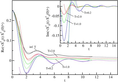
Figure 2: Numerical data (solid lines) for the autocorrelation correlation function at $\Delta=1$ and fits (dashed lines) according to Eqs. (33,34).

We begin our detailed analysis with the case $T=\infty$ where the correlation functions are real. From the results in the previous section for the free fermion point, we expect that any singular frequency-dependence will be most pronounced in this limit. Particularly interesting in this context is how the fit parameter $d$ in (33) evolves as a function of anisotropy $\Delta$ (see Table 1).

Table 1: The fit parameter $d$ as a function of anisotropy $\Delta$ at $T=\infty$ for the auto- and nearest-neighbor correlation function, respectively. A variation of the fit region gives an error estimate $\sim\pm 0.1$ in all cases. For comparison, the values $d^{ED}_{auto}$ obtained in Ref. Fabricius and McCoy, 1998 by a fit to exact diagonalization data for a $N=16$ site system are shown.

$\Delta$	$d_{auto}$	$d^{ED}_{auto}\;(N=16)$	$d_{NN}$
0.0	1.0	1.0	1.0
0.2	0.883	0.875	0.892
0.4	0.774	0.835	0.769
0.6	0.786	0.941	0.813
0.8	0.775	0.840	0.728
1.0	0.683	0.705	0.643

The numbers obtained clearly show that $d_{auto}$ for the auto- as well as $d_{NN}$ for the nearest-neighbor correlation function decrease with increasing $\Delta$. Furthermore, $d_{auto}\sim d_{NN}$ for all anisotropies. This agrees with the expectation that the power-law decay for $t\gg r$ should not depend on the spatial distance $r$. The autocorrelation function in the case $T=\infty$ has been investigated previously on the basis of exact diagonalization data for chains up to $N=16$ sites.Fabricius and McCoy (1998) There, the same fit function (33) has been used to analyze the long-time asymptotics and the exponents obtained show the same trend as a function of anisotropy (see Table 1).

The extrapolated numerical data can then be Fourier transformed. The results are shown in Fig. 3.

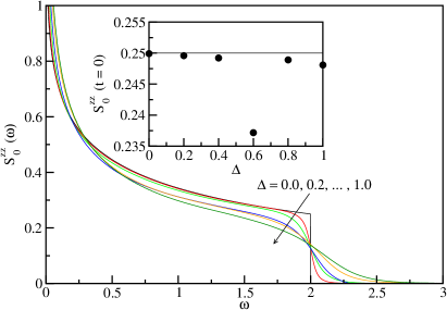
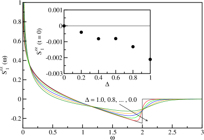
Figure 3: $S^{zz}_{0}(\omega)$ and $S^{zz}_{1}(\omega)$ for infinite temperature and different anisotropies. For $\Delta=0$ the exact results (23,24) are shown. Insets: Test of the sum rule (35) for each anisotropy. The lines denote the exact results, the dots the integrals of the numerical data.

At small frequencies both correlation functions show a power-law divergence $S^{zz}_{0,1}(\omega)\sim\omega^{-\alpha}$ with an exponent $\alpha=1-d$ and $d$ as in Table 1. In particular, $\alpha\sim 0.3-0.4$ for $\Delta=1$. Although this does not agree with the phenomenological theory of spin diffusion by BloembergenBloembergen (1949) and de Gennesde Gennes (1958) which would predict $\alpha=1/2$, it is already extremely difficult in actual NMR measurements to determine whether or not the frequency dependence is singular let alone to determine the exponent. From this perspective, we might call any kind of divergence a diffusion-like behavior. Using this terminology, we conclude that there is indeed a diffusion-like contribution to the spin-lattice relaxation rate at infinite temperature. Another point worth mentioning is the high-frequency tail in Fig. 3 for $\Delta\neq 0$. In the free fermion case all excitations contributing to the dynamical structure factor and therefore to $S^{zz}_{0,1}(\omega)$ are single particle-hole excitations. The energy of these excitations is limited by the bandwidth. For the interacting case, however, excitations of multi particle-hole type are possible which can carry arbitrarily large energies.

A test if the extrapolated real-time data indeed yield reasonable results for $S^{zz}_{0,1}(\omega)$ is provided by the sum rule

$$\int_{-\infty}^{\infty}\frac{d\omega}{2\pi}S^{zz}_{r}(\omega)=S^{zz}_{r}(t=0)\;.$$ (35)

Because $S^{zz}_{r}(-\omega)=\exp(-\beta\omega)S^{zz}_{r}(\omega)$ it is sufficient to consider the correlation functions for positive frequencies only. For the autocorrelation function $S^{zz}_{0}(t=0)=0.25$ for all anisotropies and temperatures. For $S^{zz}_{1}(\omega)$ and finite temperatures, the integrated intensity has to be compared with numerical data for the static correlation function. For infinite temperature, however, $S^{zz}_{1}(t=0)=0$. The results of this test are shown in the insets of Fig. 3.

Next, we consider finite temperatures. Based on the exact solution in the free fermion case and on what we know from field theory about the contributions from the Fermi points, it is reasonable to assume that the exponents $d$ in (33,34) are identical and that this exponent depends on anisotropy only and not on temperature. We have therefore fixed $d=(d_{auto}+d_{NN})/2$ for each anisotropy with $d_{auto},\,d_{NN}$ as in Table 1. The Fourier transform of the extrapolated data for $T=2.0$ and $T=1.0$ is shown in Fig. 4 and a check of the sum rule (35) in the insets.

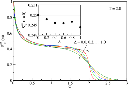
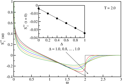
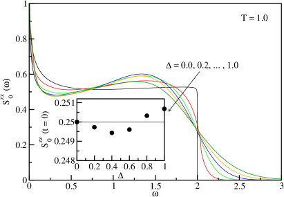
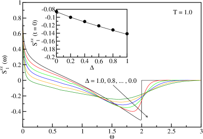
Figure 4: $S^{zz}_{0}(\omega)$ and $S^{zz}_{1}(\omega)$ for $T=2.0,\,1.0$ and different anisotropies. For $\Delta=0$ the exact results (III,20) are shown. In the insets the integrated intensities (dots) are compared with the exact result $S^{zz}_{0}(t=0)=0.25$ for the autocorrelation and with numerical data for the static nearest-neighbor correlation function (lines).

The results are qualitatively similar to the infinite temperature case. In particular, the same kind of power-law divergencies for $\omega\to 0$ and $\Delta\neq 0$ are present. Furthermore, a peak in $S^{zz}_{0}(\omega)$ starts to develop around $\omega\sim\pi/2$.

For $T<1$, however, the divergence at small frequencies gets strongly suppressed in both correlation functions (see Fig. 5) and at $T=0.2$ the singular frequency dependence can no longer be detected.

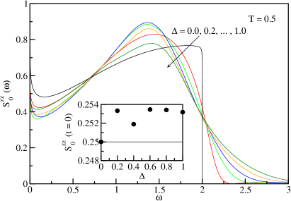
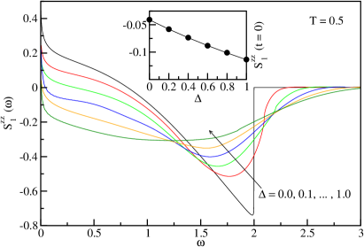
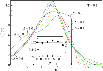
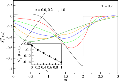
Figure 5: $S^{zz}_{0}(\omega)$ and $S^{zz}_{1}(\omega)$ for $T=0.5,\,0.2$ and different anisotropies. For $\Delta=0$ the exact results (III,20) are shown. The insets show a test of the sum rule (35).

The small kinks visible in Fig. 5 for $T=0.2$ are not of physical origin. They are most likely connected to oscillations in the real-time numerical data leading to peaks or dips in $S^{zz}_{0,1}(\omega)$ at the corresponding frequencies. $S^{zz}_{0}(\omega)$ has been studied previously for $\Delta=1$ by high-temperature series expansions and QMCStarykh et al. (1997a) as well as by a calculation of the imaginary-time correlation function using the TMRG algorithm.Naef et al. (1999) The results for this special case (see also Fig. 6(a)) presented here are very similar to the ones in these works. For example, we also see a peak at $\omega\sim\pi/2$ which increases in height with decreasing temperature and the development of a shoulder at $\omega\sim 0.7$ for $T=0.2$. Quantitatively, however, the data in Refs. Starykh et al., 1997a; Naef et al., 1999 are about a factor $2$ smaller for all frequencies. As the results here fulfill the sum rule (35) for all temperatures with good accuracy this suggests that a factor $2$ might be missing for the numerical data shown in Refs. Starykh et al., 1997a; Naef et al., 1999.

The spin-lattice relaxation rates $1/T^{a}_{1}$ and $1/T^{b}_{1}$ for $\Delta=1$ can then be obtained using (11,12) and are shown in Fig. 6.

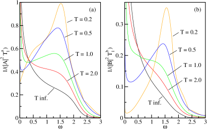
Figure 6: (a) $1/T^{a}_{1}$ for the O(2)-site and (b) $1/T^{b}_{1}$ for the O(1)-site in Sr₂CuO${}_{3}\,$.

The behavior at small frequencies seems to be similar in both cases: There is a power law divergence $\omega^{-\alpha}$ with $\alpha\sim 0.3-0.4$ at temperatures $T>J$ (remember that we set $J=1$ here), however, this divergence gets strongly suppressed at temperatures $T<J$. This suggests that the contributions to the spin-lattice relaxation rate with singular frequency dependence behave indeed similar to (21,22) found in the free fermion case.

To analyze the temperature dependence in more detail, $1/T_{1}$ for a fixed frequency $\omega\ll T$ is shown in Fig. 7.

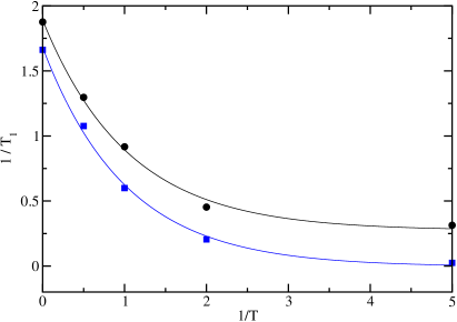
Figure 7: Temperature dependence of $1/T_{1}^{a}$ (black dots) and $1/T_{1}^{b}$ (blue squares) for $\omega=0.01$ with $A=B=1$ in Eqs. (12,11). The black line is a fit $1/T_{1}^{a}=0.27+1.62\exp(-0.96/T)$ and the blue line a fit $1/T_{1}^{b}=0.0+1.69\exp(-0.99/T)$.

The fits in Fig. 7 show that the spin-lattice relaxation rate decreases exponentially with temperature in both cases and that the scale of the exponential decrease is set by $J$ as in the free fermion case. We cannot analyze the behavior of $1/T_{1}$ at low temperatures in detail due to insufficient numerical data. However, the value $1/T_{1}^{a}(T=0.2)\approx 0.31|A|^{2}$ is close to the one predicted by the field theory formula (16) if we include logarithmic corrections to scalingStarykh et al. (1997b) yielding $1/T_{1}^{a}(T=0.2)\approx 0.27|A|^{2}$. We also note that $1/T_{1}^{a}$ only increases by about 30% when changing the temperature from $T=0.2$ to $T=0.5$. This is an indication that $1/T_{1}^{a}$ will indeed be almost constant at low temperatures as predicted by field theory. For the O(1)-site, our numerical data are consistent with $1/T_{1}^{b}\to 0$ for $T\to 0$.

V Conclusions

The purpose of this article has been to investigate if a one-dimensional Heisenberg antiferromagnet has a diffusion-like contribution to the spin-lattice relaxation rate as has been proposed in Ref. Thurber et al., 2001 based on ¹⁷O NMR experiments on Sr₂CuO${}_{3}\,$. To tackle this problem I found it useful to consider the more general $XXZ$-case which interpolates between the exactly solvable free fermion and the Heisenberg model we are interested in. For the free fermion model I have shown that a contribution to the spin-lattice relaxation rate exists which diverges logarithmically for frequency $\omega\to 0$. However, this contribution comes from the top and the bottom of the band and becomes therefore exponentially suppressed at temperatures $T<J$. The contributions from the Fermi points, on the other hand, do not show any singular frequency dependence. I then analyzed the interacting case based on real-time numerical data for the auto- and nearest-neighbor correlation functions obtained by the density-matrix renormalization group applied to transfer matrices.Sirker and Klümper (2005) The advantage of working in the real-time domain compared to imaginary-time methods is that the ill-defined analytical continuation of numerical data is circumvented. On the flip side, there is no periodicity in real-time so the numerical data have to be extrapolated in time before they can be Fourier transformed. I showed that one can do such an extrapolation using the long-time asymptotics in the free fermion case as a guide. I verified that the results obtained by this method do fulfill the sum rules with good accuracy for all anisotropies and temperatures considered. The numerical data for infinite temperature show that the logarithmic divergence of $S^{zz}_{0,1}(\omega)$ for $\omega\to 0$ in the free fermion case becomes a power-law $\sim\omega^{-\alpha}$ in the interacting case. In particular, I found $\alpha\sim 0.3-0.4$ for $\Delta=1$. With decreasing temperature these power-law divergencies become exponentially suppressed in $S^{zz}_{0}(\omega)$ as well as in $S^{zz}_{1}(\omega)$. For $\Delta=1$, I showed that the scale for this exponential suppression is still set by $J$ as in the free fermion case. The numerical data at low temperatures for $1/T_{1}^{a}$ (dominated by excitations with wave-vector $q\sim\pi$) as well as the ones for $1/T_{1}^{b}$ (dominated by excitations with wave-vector $q\sim 0$) are consistent with the field theory predictions.

What does that mean for the NMR experiments on Sr₂CuO${}_{3}\,$? First, concerning the singular frequency dependence for $\omega\to 0$, there should be no difference between measurements at the copper-, O(1)- or O(2)-site. Furthermore, a singular frequency dependence should only show up when the temperature becomes comparable to $J\approx 2000$ K. A diffusion-like contribution for $T\ll J$ as has been suggested by Thurber et al.Thurber et al. (2001) based on ¹⁷O NMR measurements at the O(1)-site cannot be explained in a pure Heisenberg model and with the hyperfine interaction being the only relevant relaxation process. However, the evidence presented in favor of such a contribution is rather weak. There is no reason to assume that the spin-lattice relaxation rate in the limit of infinite magnetic field $h$ is given by the field theory result where the effect of the magnetic field on the spin-spin correlations has been ignored. In fact, the magnetic field can only be ignored if $T\gg|h|$. Without this limiting value, however, the data in Fig. 3(d) of Ref. Thurber et al., 2001 are also consistent with having no frequency dependence at all. If that is the case, the only part of the data which is not consistent with the simple Luttinger model picture is the temperature dependence of the relaxation rate at the O(1)-site, $1/(T_{1}^{b}\,T)\sim\mbox{const}+T$ compared to $1/(T_{1}^{b}\,T)\sim\mbox{const}$ expected from field theory. As contributions from $q\sim\pi$ are strongly suppressed, this next-leading temperature dependent term most likely has to do with corrections to the simple $\delta$-peak (II) obtained from the Luttinger model for the dynamical structure factor at small $q$. From recent studies at zero temperature we know that a finite band curvature will broaden the $\delta$-peak and lead to interesting singularities at the lower and upper thresholds as well as to a high-frequency tail.Pustilnik et al. (2003, 2006); Pereira et al. (2006) At finite temperatures, spectral weight will also appear below the lower threshold. Further research, if these corrections can indeed explain the measured temperature-dependence of $1/(T_{1}^{b}\,T)$ is necessary. Finally, I want to remark that in the free fermion case the next-leading term at low temperatures is of order $T^{3}$ (see Eqs. (21,22)) and not $T^{2}$. That suggests that if a $T^{2}$-contribution exists, it should either have an amplitude which vanishes for $\Delta=0$ or otherwise the exponent has to change as a function of $\Delta$.