Spin-wave instability for parallel pumping in ferromagnetic thin films under oblique field

Abstract

Spin-wave instability for parallel pumping is studied theoretically. The spin-wave instability threshold is calculated in ferromagnetic thin films under oblique field which has an oblique angle to the film plane. The butterfly curve of the threshold usually has a cusp at a certain value of the static external field. While the static field value of the cusp point varies as the oblique angle changes, the general properties of the butterfly curve show little noteworthy change. For very thin films, however, multiple cusps of the butterfly curve can appear due to different standing spin-wave modes, which indicate a novel feature for thin films under oblique field.

,

1 Introduction

The first experiment for the parametric excitation of spin wave by parallel pumping was given by Schlöman et al. [1]. In a parallel pumping experiment, a microwave magnetic field is applied parallel to the external static field. When the microwave field amplitude $h$ exceeds a certain spin-wave instability amplitude $h_{\rm crit}$, the parametric spin-wave excitation occurs. The excited spin waves have half the pumping frequency. The $h_{\rm crit}$ curve plotted against the static field is called “butterfly curve”. The spin-wave instability for parallel pumping is often investigated for the purpose to study relaxation phenomena in ferromagnetic materials, since the instability threshold depends on the balance between the driving power and the damping of spin waves.

Theoretical studies have not been very successful to explain the instability threshold for parallel pumping: a combination of more than two equations (theories) is needed to obtain the butterfly curve. In other words, even a qualitative explanation for the butterfly curve cannot be successful so long as one tries to use only the Landau-Lifshitz (LL) equation governing the magnetization dynamics. By contrast the Suhl instability for perpendicular pumping has been well explained theoretically [2]. The Suhl instability can be described by using only the LL equation. For parallel pumping, however, the LL equation is not enough to explain the instability, and the spin-wave line width $\Delta H_{k}$ is necessary to describe the relaxation of spin-waves as well as the instability.

A typical butterfly curve for parallel pumping has a cusp at a certain external static field, which can be explained if the spin-wave line width $\Delta H_{k}$ is given. For example, Patton et al. proposed some trial $\Delta H_{k}$ functions and successfully explained butterfly curves [3]. Such a typical feature of butterfly curves usually does not depend on the shape of samples. For very thin films, however, more interesting features can appear. In fact, butterfly curves with multiple cusps were observed for $0.5$-$\mu$m yttrium iron garnet (YIG) films under in-plane external field [4]. Those cusps were due to quantized standing-wave modes across the film. It is highly desirable to develop the theory of multi-cusp butterfly curves in the case of a general oblique field.

In this paper, we examine the instability threshold for parallel pumping in ferromagnetic thin films theoretically. The butterfly curve of the threshold will be calculated in cases where the external field has an oblique angle to the film plane. For the calculation of the threshold, we use a trial $\Delta H_{k}$ function proposed by Patton et. al. [3], which was proposed originally for spherical samples but can be applied to thin films [5, 6]. For usual thin films, the butterfly curve of the threshold has a single cusp at a certain value of the static external field. We will show how the cusp shifts when the oblique angle changes. Moreover, we will reveal that multi-cusp butterfly curves can be seen for very thin films.

2 Equations of motion for the spin-wave amplitudes

The dynamics of magnetization field $\mbox{\boldmath${M}$}(\mbox{\boldmath${r}$})$ is governed by the Landau-Lifshitz (LL) equation,

$$\frac{1}{\gamma}\partial_{t}\mbox{\boldmath${M}$}=\mbox{\boldmath${M}$}\times\mbox{\boldmath${H}$}_{\rm eff}-\frac{\lambda}{M_{0}}\mbox{\boldmath${M}$}\times(\mbox{\boldmath${M}$}\times\mbox{\boldmath${H}$}_{\rm eff}).$$ (1)

Here, $\gamma$ is the gyromagnetic ratio ($\gamma<0$ for spins); $M_{0}$ is the value of the magnetization in thermal equilibrium; $\lambda$ is a damping constant parameter ($\lambda<0$ in this case); $\mbox{\boldmath${H}$}_{\rm eff}$ is the effective magnetic field:

$$\mbox{\boldmath${H}$}_{\rm eff}=D\nabla^{2}\mbox{\boldmath${M}$}+\mbox{\boldmath${H}$}^{\rm d}+\mbox{\boldmath${H}$}^{\rm a}+\mbox{\boldmath${H}$}_{0}+\mbox{\boldmath${h}$}\cos\omega t.$$ (2)

The first term comes from the exchange interaction; the third term is the anisotropy field, which is omitted below for convenience; the fourth and fifth terms are the external static and pumping fields, respectively. For parallel pumping, $\mbox{\boldmath${H}$}_{0}//\mbox{\boldmath${h}$}$ and they are parallel to the $z$ axis. The second term on right hand side of Eq. (2) is the demagnetizing filed given by the gradient of the magneto-static potential $\phi$:

$$\mbox{\boldmath${H}$}^{\rm d}=-\mbox{\boldmath${\nabla}$}\phi.$$ (3)

The magneto-static potential obeys the Poisson equation:

$$\nabla^{2}\phi=\left\{\begin{array}[]{rl}4\pi\mbox{\boldmath${\nabla}$}\cdot\mbox{\boldmath${M}$},&\mbox{inside the sample},\\ 0,&\mbox{outside the sample}.\end{array}\right.$$ (4)

The number of independent components of ${M}$ is two, since the length of the magnetization vector is invariant ($|\mbox{\boldmath${M}$}|=M_{0}$). The normalized magnetization $\mbox{\boldmath${S}$}=\mbox{\boldmath${M}$}/M_{0}$ can be represented by a point on a unit sphere. It is convenient to project the unit sphere stereographically onto a complex variable $\psi(\mbox{\boldmath${r}$},t)$ [7]:

$$\psi=\frac{S_{x}+\mathrm{i}S_{y}}{1+S_{z}},$$ (5)

where

$$S_{x}=\frac{\psi+\psi^{*}}{1+\psi\psi^{*}},\quad S_{y}=\frac{\mathrm{i}(\psi^{*}-\psi)}{1+\psi\psi^{*}},\quad S_{z}=\frac{1-\psi\psi^{*}}{1+\psi\psi^{*}}.$$ (6)

In terms of $\psi$, the LL equation (1) is rewritten as

$$\partial_{t}\psi-\mathrm{i}(1-\mathrm{i}\lambda) \gamma \left\{DM_{0}\left[\nabla^{2}\psi-\frac{2\psi^{*}(\nabla\psi)^{2}}{1+\psi\psi^{*}}\right]-\frac{1}{2}(1-\psi^{2})\partial_{x}\phi\right.$$ (7)

$$- \left.\frac{\rm i}{2}(1+\psi^{*2})\partial_{y}\phi+(\partial_{z}\phi-H_{0}-h\cos\omega t)\psi\right\}=0.$$

Inside the sample, $\phi$ satisfies

$$\nabla^{2}\phi = \frac{4\pi M_{0}}{(1+\psi\psi^{*})^{2}}\left\{(1-\psi^{*2})\partial_{x}\psi+(1-\psi^{2})\partial_{x}\psi^{*}\right.$$ (8)

$$+ \left.\mathrm{i}[(1+\psi^{2})\partial_{y}\psi^{*}-(1+\psi^{*2})\partial_{y}\psi]-2(\psi\partial_{z}\psi^{*}+\psi^{*}\partial_{z}\psi)\right\}.$$

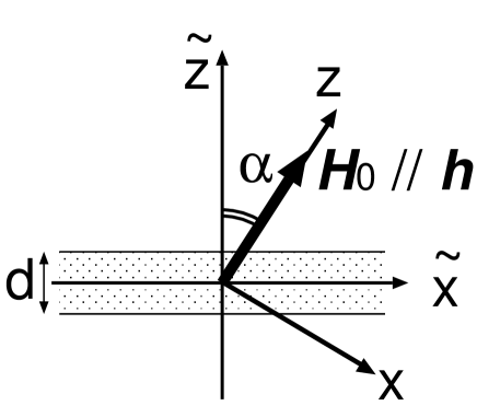
Figure 1: Schematic picture of sample setting. The sample extends on the $\tilde{x}$-$\tilde{y}$ plane. The $z$ axis corresponds to the direction of the external filed and has an angle $\alpha$ to the $\tilde{z}$ axis.

Now let us consider the boundary conditions, which affect the demagnetizing field. We assume a film of thickness $d$ infinitely extended in the $\tilde{x}$-$\tilde{y}$ plane as shown in Fig. 1. The external field is at an angle $\alpha$ to the $\tilde{z}$ axis and corresponds to the $z$ axis. We assume unpinned surface spins, which satisfy Neumann-like boundary conditions,

$$\partial_{\tilde{z}}\mbox{\boldmath${S}$}|_{\tilde{z}=\pm d/2}=0,$$ (9)

namely,

$$\left.\frac{\partial}{\partial\tilde{z}}\psi\right|_{\tilde{z}=\pm d/2}=\left.\frac{\partial}{\partial\tilde{z}}\psi^{*}\right|_{\tilde{z}=\pm d/2}=0.$$ (10)

Before proceeding to the linear instability of spin waves, we introduce the following dimensionless time and space units [8]:

$$t\to\frac{t}{4\pi|\gamma|M_{0}},\quad\mbox{\boldmath${r}$}\to\mbox{\boldmath${r}$}d.$$ (11)

Then we obtain the linearized equations of motion corresponding to Eqs. (7) and (8):

$$\partial_{t}\psi+\mathrm{i}(1-\mathrm{i}\lambda)\left[l^{2}\nabla^{2}\psi-\frac{1}{2}(\partial_{x}+\mathrm{i}\partial_{y})\Phi+(\partial_{z}\Phi-\omega_{H}-\omega_{h}\cos\omega_{\rm p}t)\psi\right]=0,$$ (12)

$$\nabla^{2}\Phi=(\partial_{x}-\mathrm{i}\partial_{y})\psi+(\partial_{x}+\mathrm{i}\partial_{y})\psi^{*}\quad\mbox{when $-\frac{1}{2}<\tilde{z}<\frac{1}{2}$},$$ (13)

where

$$l^{2}=\frac{D}{4\pi d^{2}},\quad\Phi=\frac{\phi}{4\pi M_{0}d},\quad\omega_{H}=\frac{H_{0}}{4\pi M_{0}},\quad\omega_{h}=\frac{h}{4\pi M_{0}},\quad\omega_{\rm p}=\frac{\omega}{4\pi M_{0}|\gamma|}.$$ (14)

Now we consider the undriven case (i.e., $\omega_{h}=0$), and expand $\psi(\mbox{\boldmath${r}$},t)$ and $\psi^{*}(\mbox{\boldmath${r}$},t)$ so that they fulfills the boundary conditions (10). For even modes, $\tilde{k}_{z}=2m\pi$ ($m$: integer),

$$\psi(\tilde{\mbox{\boldmath${r}$}},t) = \sum_{\tilde{\mbox{\boldmath${\scriptstyle k}$}}}a_{\tilde{\mbox{\boldmath${\scriptstyle k}$}}}(t)\e^{\mathrm{i}(\tilde{k}_{x}\tilde{x}+\tilde{k}_{y}\tilde{y})}\cos\tilde{k}_{z}\tilde{z}$$

$$\psi^{*}(\tilde{\mbox{\boldmath${r}$}},t) = \sum_{\tilde{\mbox{\boldmath${\scriptstyle k}$}}}a^{*}_{-\tilde{\mbox{\boldmath${\scriptstyle k}$}}}(t)\e^{\mathrm{i}(\tilde{k}_{x}\tilde{x}+\tilde{k}_{y}\tilde{y})}\cos\tilde{k}_{z}\tilde{z}.$$ (15)

For odd modes, $\tilde{k}_{z}=(2m+1)\pi$ ($m$: integer),

$$\psi(\tilde{\mbox{\boldmath${r}$}},t) = \sum_{\tilde{\mbox{\boldmath${\scriptstyle k}$}}}a_{\tilde{\mbox{\boldmath${\scriptstyle k}$}}}(t)\e^{\mathrm{i}(\tilde{k}_{x}\tilde{x}+\tilde{k}_{y}\tilde{y})}\sin\tilde{k}_{z}\tilde{z}$$

$$\psi^{*}(\tilde{\mbox{\boldmath${r}$}},t) = -\sum_{\tilde{\mbox{\boldmath${\scriptstyle k}$}}}a^{*}_{-\tilde{\mbox{\boldmath${\scriptstyle k}$}}}(t)\e^{\mathrm{i}(\tilde{k}_{x}\tilde{x}+\tilde{k}_{y}\tilde{y})}\sin\tilde{k}_{z}\tilde{z}.$$ (16)

Here, $\tilde{k}_{x}=k_{x}\cos\alpha+k_{z}\sin\alpha$, $\tilde{k}_{y}=k_{y}$, and $\tilde{k}_{z}=k_{z}\cos\alpha-k_{x}\sin\alpha$. Using the expansions (15) and (16), we obtain solutions of Eq. (13): for even modes,

$$\Phi(\tilde{\mbox{\boldmath${r}$}}) = -\sum_{\tilde{\mbox{\boldmath${\scriptstyle k}$}}}\frac{\e^{\mathrm{i}(\tilde{k}_{x}\tilde{x}+\tilde{k}_{y}\tilde{y})}}{\tilde{k}^{2}}\left[\mathrm{i}(\tilde{k}_{-}a_{\tilde{\mbox{\boldmath${\scriptstyle k}$}}}+\tilde{k}_{+}a^{*}_{-\tilde{\mbox{\boldmath${\scriptstyle k}$}}})\left\{\cos\tilde{k}_{z}\tilde{z}-(-1)^{m}\e^{-\tilde{k}_{\perp}/2}\cosh\tilde{k}_{\perp}\tilde{z}\right\}\right.$$ (17)

$$+ \left.\tilde{k}_{z}\sin\alpha\cdot(a_{\tilde{\mbox{\boldmath${\scriptstyle k}$}}}+a^{*}_{-\tilde{\mbox{\boldmath${\scriptstyle k}$}}})\left\{\sin\tilde{k}_{z}\tilde{z}-(-1)^{m}\e^{-\tilde{k}_{\perp}/2}(\tilde{k}_{z}/\tilde{k}_{\perp})\sinh\tilde{k}_{\perp}\tilde{z}\right\}\right],$$

for odd modes,

$$\Phi(\tilde{\mbox{\boldmath${r}$}}) = -\sum_{\tilde{\mbox{\boldmath${\scriptstyle k}$}}}\frac{\e^{\mathrm{i}(\tilde{k}_{x}\tilde{x}+\tilde{k}_{y}\tilde{y})}}{\tilde{k}^{2}}\left[\mathrm{i}(\tilde{k}_{-}a_{\tilde{\mbox{\boldmath${\scriptstyle k}$}}}-\tilde{k}_{+}a^{*}_{-\tilde{\mbox{\boldmath${\scriptstyle k}$}}})\left\{\sin\tilde{k}_{z}\tilde{z}-(-1)^{m}\e^{-\tilde{k}_{\perp}/2}\sinh\tilde{k}_{\perp}\tilde{z}\right\}\right.$$ (18)

$$- \left.\tilde{k}_{z}\sin\alpha\cdot(a_{\tilde{\mbox{\boldmath${\scriptstyle k}$}}}-a^{*}_{-\tilde{\mbox{\boldmath${\scriptstyle k}$}}})\left\{\cos\tilde{k}_{z}\tilde{z}+(-1)^{m}\e^{-\tilde{k}_{\perp}/2}(\tilde{k}_{z}/\tilde{k}_{\perp})\cosh\tilde{k}_{\perp}\tilde{z}\right\}\right],$$

where $\tilde{k}_{+}=\tilde{k}_{x}\cos\alpha+\mathrm{i}\tilde{k}_{y}$, $\tilde{k}_{-}=\tilde{k}_{x}\cos\alpha-\mathrm{i}\tilde{k}_{y}$ and $\tilde{k}_{\perp}=\sqrt{\tilde{k}_{x}^{2}+\tilde{k}_{y}^{2}}$. The detailed derivation of these solutions is shown in Appendix A. Here we approximate $\partial_{z}\Phi=-H^{\rm d}_{z}/4\pi M_{0}$ with the value of uniform magnetization, $\mbox{\boldmath${k}$}=0$: $H^{\rm d}_{z}=H^{\rm d}_{\tilde{x}}\sin\alpha+H^{\rm d}_{\tilde{z}}\cos\alpha=-4\pi(N_{\tilde{x}}M_{\tilde{x}}\sin\alpha+N_{\tilde{z}}M_{\tilde{z}}\cos\alpha)$, where $N_{\tilde{x}}$ and $N_{\tilde{z}}$ are demagnetizing factors. In this case, $N_{\tilde{x}}=N_{\tilde{y}}=0$ and $N_{\tilde{z}}=1$ . Assuming $M_{z}\simeq M_{0}$, namely, $M_{\tilde{z}}\simeq M_{0}\cos\alpha$, we obtain $\partial_{z}\Phi=-H^{\rm d}_{z}/4\pi M_{0}=\cos^{2}\alpha$. Then Eq. (12) for $\omega_{h}=0$ is rewritten as

$$\partial_{t}\psi+\mathrm{i}(1-\mathrm{i}\lambda)\left[l^{2}\nabla^{2}\psi-\frac{1}{2}(\cos\alpha\partial_{\tilde{x}}+\mathrm{i}\partial_{\tilde{y}}-\sin\alpha\partial_{\tilde{z}})\Phi+(\cos^{2}\alpha-\omega_{H})\psi\right]=0.$$ (19)

Combining Eqs. (15)-(19), we obtain

$$\partial_{t}a_{\mbox{\boldmath${\scriptstyle k}$}}+\mathrm{i}(1-\mathrm{i}\lambda)A_{\mbox{\boldmath${\scriptstyle k}$}}a_{\mbox{\boldmath${\scriptstyle k}$}}+\mathrm{i}(1-\mathrm{i}\lambda)B_{\mbox{\boldmath${\scriptstyle k}$}}a^{*}_{-\mbox{\boldmath${\scriptstyle k}$}}=0,$$ (20)

where

$$A_{\mbox{\boldmath${\scriptstyle k}$}}=C_{\mbox{\boldmath${\scriptstyle k}$}}+\mathrm{Re}\tilde{C_{\mbox{\boldmath${\scriptstyle k}$}}},\quad B_{\mbox{\boldmath${\scriptstyle k}$}}=(-1)^{n}\left(D_{\mbox{\boldmath${\scriptstyle k}$}}\e^{2\mathrm{i}\varphi_{\mbox{\boldmath${\scriptscriptstyle k}$}}}+\tilde{C_{\mbox{\boldmath${\scriptstyle k}$}}}\right).$$ (21)

Here, $n$ is an integer, $\cos\varphi_{\mbox{\boldmath${\scriptstyle k}$}}=k_{x}/k_{\perp}$, $\sin\varphi_{\mbox{\boldmath${\scriptstyle k}$}}=k_{y}/k_{\perp}$, $k_{\perp}=\sqrt{k_{x}^{2}+k_{y}^{2}}$, and

$$C_{\mbox{\boldmath${\scriptstyle k}$}} = \cos^{2}\alpha-l^{2}k^{2}-\omega_{H}-\frac{1}{2}f_{\mbox{\boldmath${\scriptstyle k}$}}\sin^{2}\theta_{\mbox{\boldmath${\scriptstyle k}$}},$$

$$\tilde{C_{\mbox{\boldmath${\scriptstyle k}$}}} = -\frac{\tilde{k}_{z}}{k^{2}}\sin\alpha\left(k_{\perp}\e^{\mathrm{i}\varphi_{\mbox{\boldmath${\scriptscriptstyle k}$}}}+\tilde{k}_{z}\sin\alpha\right)f_{\mbox{\boldmath${\scriptstyle k}$}},$$

$$D_{\mbox{\boldmath${\scriptstyle k}$}} = -\frac{1}{2}f_{\mbox{\boldmath${\scriptstyle k}$}}\sin^{2}\theta_{\mbox{\boldmath${\scriptstyle k}$}},$$

$$f_{\mbox{\boldmath${\scriptstyle k}$}} = 1-(2-\delta_{0n})\left(1-\exp\left[-\sqrt{k^{2}-\tilde{k}_{z}^{2}}\right]\right)\frac{\sqrt{k^{2}-\tilde{k}_{z}^{2}}}{k^{2}},$$ (22)

$$\sin\theta_{\mbox{\boldmath${\scriptstyle k}$}}=\frac{k_{\perp}}{k},\quad\tilde{k}_{z}=\pi n.$$

The detailed derivation is given in Appendix B.

Equation (20) represents two coupled harmonic oscillators $a_{\mbox{\boldmath${\scriptstyle k}$}}$, $a^{*}_{-\mbox{\boldmath${\scriptstyle k}$}}$. We diagonalize Eq. (20) by means of the Holstein-Primakoff transformation:

$$a_{\mbox{\boldmath${\scriptstyle k}$}} = \nu_{\mbox{\boldmath${\scriptstyle k}$}}b_{\mbox{\boldmath${\scriptstyle k}$}}-\mu_{\mbox{\boldmath${\scriptstyle k}$}}b^{*}_{-\mbox{\boldmath${\scriptstyle k}$}}$$

$$a^{*}_{-\mbox{\boldmath${\scriptstyle k}$}} = \nu_{\mbox{\boldmath${\scriptstyle k}$}}b^{*}_{-\mbox{\boldmath${\scriptstyle k}$}}-\mu^{*}_{\mbox{\boldmath${\scriptstyle k}$}}b_{\mbox{\boldmath${\scriptstyle k}$}},$$ (23)

where

$$\nu_{\mbox{\boldmath${\scriptstyle k}$}} = \cosh\frac{\chi_{\mbox{\boldmath${\scriptstyle k}$}}}{2},$$

$$\mu_{\mbox{\boldmath${\scriptstyle k}$}} = \e^{\mathrm{i}\beta_{\mbox{\boldmath${\scriptscriptstyle k}$}}}\sinh\frac{\chi_{\mbox{\boldmath${\scriptstyle k}$}}}{2},$$

$$\cosh\chi_{\mbox{\boldmath${\scriptstyle k}$}} = \frac{\left|C_{\mbox{\boldmath${\scriptstyle k}$}}+\mathrm{Re}\tilde{C_{\mbox{\boldmath${\scriptstyle k}$}}}\right|}{\left[(C_{\mbox{\boldmath${\scriptstyle k}$}}+\mathrm{Re}\tilde{C_{\mbox{\boldmath${\scriptstyle k}$}}})^{2}-(1+\lambda^{2})\left|D_{\mbox{\boldmath${\scriptstyle k}$}}\e^{2\mathrm{i}\varphi_{\mbox{\boldmath${\scriptscriptstyle k}$}}}+\tilde{C_{\mbox{\boldmath${\scriptstyle k}$}}}\right|^{2}\right]^{1/2}}.$$ (24)

Substituting Eq. (23) into Eq. (20), we obtain

$$\partial_{t}b_{\mbox{\boldmath${\scriptstyle k}$}}-\mathrm{i}(\omega_{\mbox{\boldmath${\scriptstyle k}$}}+\mathrm{i}\eta_{\mbox{\boldmath${\scriptstyle k}$}})b_{\mbox{\boldmath${\scriptstyle k}$}}=0,$$ (25)

where

$$\omega_{\mbox{\boldmath${\scriptstyle k}$}}^{2} = (C_{\mbox{\boldmath${\scriptstyle k}$}}+\mathrm{Re}\tilde{C_{\mbox{\boldmath${\scriptstyle k}$}}})^{2}-(1+\lambda^{2})\left|D_{\mbox{\boldmath${\scriptstyle k}$}}\e^{2\mathrm{i}\varphi_{\mbox{\boldmath${\scriptscriptstyle k}$}}}+\tilde{C_{\mbox{\boldmath${\scriptstyle k}$}}}\right|^{2},$$ (26)

$$\eta_{\mbox{\boldmath${\scriptstyle k}$}} = \lambda(C_{\mbox{\boldmath${\scriptstyle k}$}}+\mathrm{Re}\tilde{C_{\mbox{\boldmath${\scriptstyle k}$}}})$$ (27)

Equations (26) and (27) express the dispersion relation and a damping rate, respectively.

3 The instability threshold

Now we consider the case where the microwave field $\mbox{\boldmath${h}$}\cos\omega t$ is applied. The equation of motion of $a_{\mbox{\boldmath${\scriptstyle k}$}}$ corresponding to Eq. (20) is

$$\partial_{t}a_{\mbox{\boldmath${\scriptstyle k}$}}+\mathrm{i}(1-\mathrm{i}\lambda)A_{\mbox{\boldmath${\scriptstyle k}$}}a_{\mbox{\boldmath${\scriptstyle k}$}}+\mathrm{i}(1-\mathrm{i}\lambda)B_{\mbox{\boldmath${\scriptstyle k}$}}a^{*}_{-\mbox{\boldmath${\scriptstyle k}$}}-\mathrm{i}(1-\mathrm{i}\lambda)\omega_{h}\cos\omega_{\rm p}t\cdot a_{\mbox{\boldmath${\scriptstyle k}$}}=0.$$ (28)

After the the Holstein-Primakoff transformation (23), we substitute the following equations into Eq. (28),

$$b_{\mbox{\boldmath${\scriptstyle k}$}}(t) = b^{o}_{\mbox{\boldmath${\scriptstyle k}$}}(t)\exp[\mathrm{i}(\omega_{\rm p}/2)t-\eta_{\mbox{\boldmath${\scriptstyle k}$}}t],$$

$$b^{*}_{-\mbox{\boldmath${\scriptstyle k}$}}(t) = b^{o*}_{-\mbox{\boldmath${\scriptstyle k}$}}(t)\exp[-\mathrm{i}(\omega_{\rm p}/2)t-\eta_{\mbox{\boldmath${\scriptstyle k}$}}t],$$ (29)

since the resonance occurs at $\omega_{\mbox{\boldmath${\scriptstyle k}$}}=\omega_{\rm p}/2$. Then the slowly-varying variable $b^{o}_{\mbox{\boldmath${\scriptstyle k}$}}$ satisfies

$$\partial_{t}^{2}b^{o}_{\mbox{\boldmath${\scriptstyle k}$}}+\left[\left(\omega_{\mbox{\boldmath${\scriptstyle k}$}}-\frac{\omega_{\rm p}}{2}\right)^{2}-\left|\rho_{\mbox{\boldmath${\scriptstyle k}$}}\right|^{2}\right]b^{o}_{\mbox{\boldmath${\scriptstyle k}$}}=0,$$ (30)

where

$$\left|\rho_{\mbox{\boldmath${\scriptstyle k}$}}\right|=\omega_{h}\sqrt{1+\lambda^{2}}\frac{\left|D_{\mbox{\boldmath${\scriptstyle k}$}}\e^{2\mathrm{i}\varphi_{\mbox{\boldmath${\scriptscriptstyle k}$}}}+\tilde{C_{\mbox{\boldmath${\scriptstyle k}$}}}\right|}{2\omega_{\mbox{\boldmath${\scriptstyle k}$}}}.$$ (31)

Therefore, the exponentially increasing solution for $b_{\mbox{\boldmath${\scriptstyle k}$}}$ is

$$b_{\mbox{\boldmath${\scriptstyle k}$}}\propto\exp\left[\left(\left|\rho_{\mbox{\boldmath${\scriptstyle k}$}}\right|-\eta_{\mbox{\boldmath${\scriptstyle k}$}}\right)t+\mathrm{i}(\omega_{\rm p}/2)t\right],$$ (32)

where

$$\left|\rho_{\mbox{\boldmath${\scriptstyle k}$}}\right|>\eta_{\mbox{\boldmath${\scriptstyle k}$}}.$$ (33)

The instability threshold $\omega_{h}^{\rm crit}$ is now given as

$$\omega_{h}^{\rm crit}=\frac{\omega_{\rm p}}{\sqrt{1+\lambda^{2}}}\min_{\mbox{\boldmath${\scriptstyle k}$}}\left\{\frac{\eta_{\mbox{\boldmath${\scriptstyle k}$}}}{\left|D_{\mbox{\boldmath${\scriptstyle k}$}}\e^{2\mathrm{i}\varphi_{\mbox{\boldmath${\scriptscriptstyle k}$}}}+\tilde{C_{\mbox{\boldmath${\scriptstyle k}$}}}\right|}\right\}.$$ (34)

The threshold, Eq. (34), is obtained by using only the LL equation, but cannot explain the experimentally-observed instability threshold for parallel pumping. In fact, Eq. (34) proves to give an instability curve totally different from the real butterfly curve. Since the relaxation phenomenon is essentially nonlinear one, the linearizion analysis is not sufficient to discuss the instability threshold. The problem is beyond the purpose of this paper, and it will be discussed in a forthcoming paper [9]. This difficulty, however, can be overcome by replacing the damping rate $\eta_{\mbox{\boldmath${\scriptstyle k}$}}$ by a suitable spin-wave line width. Using the spin-wave line width $\Delta H_{\mbox{\boldmath${\scriptstyle k}$}}$, we rewrite Eq. (34) as

$$\omega_{h}^{\rm crit}=\omega_{\rm p}\min_{\mbox{\boldmath${\scriptstyle k}$}}\left\{\frac{\Delta H_{\mbox{\boldmath${\scriptstyle k}$}}}{\left|D_{\mbox{\boldmath${\scriptstyle k}$}}\e^{2\mathrm{i}\varphi_{\mbox{\boldmath${\scriptscriptstyle k}$}}}\tilde{C_{\mbox{\boldmath${\scriptstyle k}$}}}\right|}\right\}.$$ (35)

Here we adopt a simple trial $\Delta H_{\mbox{\boldmath${\scriptstyle k}$}}$ function [3],

$$\Delta H_{\mbox{\boldmath${\scriptstyle k}$}}=A_{0}+A_{1}\sin^{2}(2\theta_{k})+A_{2}k,$$ (36)

where $A_{0}$, $A_{1}$ and $A_{2}$ are adjustable parameters.

4 Butterfly curves

Typical butterfly curves of the threshold $\omega_{h}^{\rm crit}$ have a cusp at a certain static field: as the static field increasing, $\omega_{h}^{\rm crit}$ decreases below the cusp point and increases above that. For static fields below the cusp point, the minimum threshold modes corresponds to a spin wave propagating with $\theta_{\mbox{\boldmath${\scriptstyle k}$}}=\pi/2$. As the static field increases, the wave vector $k$ of the threshold modes decreases, and $k\simeq 0$ at the cusp. For static fields above the cusp point, the wave number remains at $k\simeq 0$ and $\theta_{\mbox{\boldmath${\scriptstyle k}$}}$ decreases from $\pi/2$ to $0$.

Figure 2: Theoretical butterfly curves for $d=15\mu$m for some values of the oblique angle $\alpha$.

Figure 2 shows theoretical butterfly curves calculated by using Eqs. (35) and (36). The material parameters used in the calculation are typical values for yttrium iron garnet (YIG) materials: $|\gamma|=1.77\times 10^{7}$rad/(s$\cdot$Oe), $4\pi M_{0}=1.75\times 10^{3}$Oe, $D=5.4\times 10^{-9}$Oe$\cdot$cm²/rad². The other parameters are as follows: $\omega/(2\pi)=9.5\times 10^{9}$Hz, $d=15\mu$m, $A_{0}=3.0\times 10^{-2}/(4\pi M_{0})$, $A_{1}/A_{0}=0.4$, $A_{2}/A_{0}=3.0\times 10^{-4}/d$. We calculate the static field value for the cusp point with $k=0$ and $\theta_{\mbox{\boldmath${\scriptstyle k}$}}$ in a bulk approximation: we assume $f_{\mbox{\boldmath${\scriptstyle k}$}}=1$ in Eq. (22). Setting $\omega_{\mbox{\boldmath${\scriptstyle k}$}}=\omega_{\rm p}/2$ in Eq. (26), we obtain the static field for the cusp point

$$\omega_{H}^{\rm crit}=\cos^{2}\alpha-\frac{1}{2}+\frac{1}{2}\sqrt{\omega_{\rm p}^{2}+1}.$$ (37)

While the cusp point shifts to lower static fields as the oblique angle $\alpha$ increases, the typical shape of curves is found to show little noteworthy change.

In some cases, however, curious butterfly curves can emerge.

Figure 3: Theoretical butterfly curve for $d=5\mu$m. The external field is applied parallel to the film plane.

Figure 3 is a theoretical butterfly curve for the case of $d=5\mu$m and $\alpha=\pi/2$. The other parameters used in the calculation are the same as used in Fig. 2. There appear multiple cusps in the low field region of the butterfly curve. These cusps are due to different standing spin-wave modes across the film thickness. Let us recall that the $\tilde{z}$ component of wave vectors are quantized. Effects of quantization are essential when the boundary conditions become important. Comparing the results in Figs. 2 and 3, one may say multi-cusp feature of a butterfly curve can be seen when the thickness of a film is very small. This finding is supported by some experimental studies [4, 5]. In Ref. [5], a standard butterfly curve of the instability was shown for 15.9-$\mu$m-thick yttrium iron garnet (YIG) film under in-plane external field. However, in Ref. [4], multiple butterfly curves appeared for a YIG film under in-plane external field. The difference between the two is just the thickness. The thickness of the film in Ref. [4] was 0.5$\mu$m.

5 Discussion

We have revealed how butterfly curves depend on the oblique angle between the external field and the film plane. We have calculated theoretical butterfly curves by using the LL equation together with the spin-wave line width $\Delta H_{k}$. The calculation was performed under the assumption that parameters $A_{0}$, $A_{1}$ and $A_{2}$ for $\Delta H_{k}$ do not depend on the oblique angle. These parameters were originally introduced to fit a theoretical butterfly curve to experimental data [3], and might depend on the oblique angle.

We have also shown qualitative features of the novel aspect of butterfly curves with multiple cusps for parallel pumping. Those multi-cusp curves come from quantized standing-wave modes across the film. However, it is not clear how such cusps appear, since there remains an ambiguity about how to evaluate $A_{0}$, $A_{1}$ and $A_{2}$. Figure 3 is one of possible theoretical curves. To proceed to quantitative evaluations, the experimental test is highly desirable to confirm the features predicted here.

Appendix A Demagnetization field

First, we should use the $(\tilde{x},\tilde{y},\tilde{z})$ coordinate system rather than $(x,y,z)$ to use Eqs. (15) and (16) in the Poisson equation (4), and employ the transformation: $\nabla^{2}\to\tilde{\nabla}^{2}$, $\partial_{x}\to\cos\alpha\partial_{\tilde{x}}-\sin\alpha\partial_{\tilde{z}}$. We consider only the case of $-\frac{1}{2}<\tilde{z}<\frac{1}{2}$. For even modes, $\tilde{k}_{z}=2m\pi$ ($m$: integer), the Poisson equation is rewritten as

$$\tilde{\nabla}^{2}\Phi=\sum_{\tilde{\mbox{\boldmath${\scriptstyle k}$}}}\e^{\mathrm{i}(\tilde{k}_{x}\tilde{x}+\tilde{k}_{y}\tilde{y})} \left[(\mathrm{i}\tilde{k}_{-}\cos\tilde{k}_{z}\tilde{z}+\tilde{k}_{z}\sin\alpha\sin\tilde{k}_{z}\tilde{z})a_{\mbox{\boldmath${\scriptstyle k}$}}\right.$$ (38)

$$+ \left.(\mathrm{i}\tilde{k}_{+}\cos\tilde{k}_{z}\tilde{z}+\tilde{k}_{z}\sin\alpha\sin\tilde{k}_{z}\tilde{z})a^{*}_{-\mbox{\boldmath${\scriptstyle k}$}}\right],$$

where $\tilde{k}_{+}=\tilde{k}_{x}\cos\alpha+\mathrm{i}\tilde{k}_{y}$ and $\tilde{k}_{-}=\tilde{k}_{x}\cos\alpha-\mathrm{i}\tilde{k}_{y}$. For odd modes, $\tilde{k}_{z}=(2m+1)\pi$ ($m$: integer),

$$\tilde{\nabla}^{2}\Phi=\sum_{\tilde{\mbox{\boldmath${\scriptstyle k}$}}}\e^{\mathrm{i}(\tilde{k}_{x}\tilde{x}+\tilde{k}_{y}\tilde{y})} \left[(\mathrm{i}\tilde{k}_{-}\sin\tilde{k}_{z}\tilde{z}-\tilde{k}_{z}\sin\alpha\cos\tilde{k}_{z}\tilde{z})a_{\mbox{\boldmath${\scriptstyle k}$}}\right.$$ (39)

$$- \left.(\mathrm{i}\tilde{k}_{+}\sin\tilde{k}_{z}\tilde{z}-\tilde{k}_{z}\sin\alpha\cos\tilde{k}_{z}\tilde{z})a^{*}_{-\mbox{\boldmath${\scriptstyle k}$}}\right].$$

Here we note a well known fact: the Poisson equation,

$$\nabla^{2}\phi(\mbox{\boldmath${r}$})=-4\pi\rho(\mbox{\boldmath${r}$}),$$ (40)

has the solution as

$$\phi(\mbox{\boldmath${r}$})=\int\frac{\rho(\mbox{\boldmath${r}$}^{\prime})\d\mbox{\boldmath${V}$}^{\prime}}{|\mbox{\boldmath${r}$}^{\prime}-\mbox{\boldmath${r}$}|}.$$ (41)

Applying Eq. (41), we obtain the solution of Eqs. (38) and (39): for even modes,

$$\Phi(\tilde{\mbox{\boldmath${r}$}})=-\frac{1}{4\pi} \sum_{\tilde{\mbox{\boldmath${\scriptstyle k}$}}} \left\{\mathrm{i}(\tilde{k}_{-}a_{\tilde{\mbox{\boldmath${\scriptstyle k}$}}}+\tilde{k}_{+}a^{*}_{-\tilde{\mbox{\boldmath${\scriptstyle k}$}}})\int\frac{\d\tilde{\mbox{\boldmath${V}$}}^{\prime}}{|\tilde{\mbox{\boldmath${r}$}}^{\prime}-\tilde{\mbox{\boldmath${r}$}}|}\e^{\mathrm{i}(\tilde{k}_{x}\tilde{x}^{\prime}+\tilde{k}_{y}\tilde{y}^{\prime})}\cos\tilde{k}_{z}\tilde{z}^{\prime}\right.$$ (42)

$$+ \left.\tilde{k}_{z}\sin\alpha\cdot(a_{\tilde{\mbox{\boldmath${\scriptstyle k}$}}}+a^{*}_{-\tilde{\mbox{\boldmath${\scriptstyle k}$}}})\int\frac{\d\tilde{\mbox{\boldmath${V}$}}^{\prime}}{|\tilde{\mbox{\boldmath${r}$}}^{\prime}-\tilde{\mbox{\boldmath${r}$}}|}\e^{\mathrm{i}(\tilde{k}_{x}\tilde{x}^{\prime}+\tilde{k}_{y}\tilde{y}^{\prime})}\sin\tilde{k}_{z}\tilde{z}^{\prime}\right\};$$

for odd modes,

$$\Phi(\tilde{\mbox{\boldmath${r}$}})=-\frac{1}{4\pi} \sum_{\tilde{\mbox{\boldmath${\scriptstyle k}$}}} \left\{\mathrm{i}(\tilde{k}_{-}a_{\tilde{\mbox{\boldmath${\scriptstyle k}$}}}-\tilde{k}_{+}a^{*}_{-\tilde{\mbox{\boldmath${\scriptstyle k}$}}})\int\frac{\d\tilde{\mbox{\boldmath${V}$}}^{\prime}}{|\tilde{\mbox{\boldmath${r}$}}^{\prime}-\tilde{\mbox{\boldmath${r}$}}|}\e^{\mathrm{i}(\tilde{k}_{x}\tilde{x}^{\prime}+\tilde{k}_{y}\tilde{y}^{\prime})}\sin\tilde{k}_{z}\tilde{z}^{\prime}\right.$$ (43)

$$- \left.\tilde{k}_{z}\sin\alpha\cdot(a_{\tilde{\mbox{\boldmath${\scriptstyle k}$}}}-a^{*}_{-\tilde{\mbox{\boldmath${\scriptstyle k}$}}})\int\frac{\d\tilde{\mbox{\boldmath${V}$}}^{\prime}}{|\tilde{\mbox{\boldmath${r}$}}^{\prime}-\tilde{\mbox{\boldmath${r}$}}|}\e^{\mathrm{i}(\tilde{k}_{x}\tilde{x}^{\prime}+\tilde{k}_{y}\tilde{y}^{\prime})}\cos\tilde{k}_{z}\tilde{z}^{\prime}\right\}.$$

After integration, Eqs. (42) and (43) become

$$\Phi(\tilde{\mbox{\boldmath${r}$}})= - \sum_{\tilde{\mbox{\boldmath${\scriptstyle k}$}}}\frac{\e^{\mathrm{i}(\tilde{k}_{x}\tilde{x}+\tilde{k}_{y}\tilde{y})}}{\tilde{k}^{2}}\left\{\mathrm{i}(\tilde{k}_{-}a_{\tilde{\mbox{\boldmath${\scriptstyle k}$}}}+\tilde{k}_{+}a^{*}_{-\tilde{\mbox{\boldmath${\scriptstyle k}$}}})\left[\cos\tilde{k}_{z}\tilde{z}-(-1)^{m}\e^{-\tilde{k}_{\perp}/2}\cosh\tilde{k}_{\perp}\tilde{z}\right]\right.$$ (44)

$$+ \left.\tilde{k}_{z}\sin\alpha\cdot(a_{\tilde{\mbox{\boldmath${\scriptstyle k}$}}}+a^{*}_{-\tilde{\mbox{\boldmath${\scriptstyle k}$}}})\left[\sin\tilde{k}_{z}\tilde{z}-(-1)^{m}\e^{-\tilde{k}_{\perp}/2}\frac{\tilde{k}_{z}}{\tilde{k}_{\perp}}\sinh\tilde{k}_{\perp}\tilde{z}\right]\right\},$$

and

$$\Phi(\tilde{\mbox{\boldmath${r}$}})= - \sum_{\tilde{\mbox{\boldmath${\scriptstyle k}$}}}\frac{\e^{\mathrm{i}(\tilde{k}_{x}\tilde{x}+\tilde{k}_{y}\tilde{y})}}{\tilde{k}^{2}}\left\{\mathrm{i}(\tilde{k}_{-}a_{\tilde{\mbox{\boldmath${\scriptstyle k}$}}}-\tilde{k}_{+}a^{*}_{-\tilde{\mbox{\boldmath${\scriptstyle k}$}}})\left[\sin\tilde{k}_{z}\tilde{z}-(-1)^{m}\e^{-\tilde{k}_{\perp}/2}\sinh\tilde{k}_{\perp}\tilde{z}\right]\right.$$ (45)

$$- \left.\tilde{k}_{z}\sin\alpha\cdot(a_{\tilde{\mbox{\boldmath${\scriptstyle k}$}}}-a^{*}_{-\tilde{\mbox{\boldmath${\scriptstyle k}$}}})\left[\cos\tilde{k}_{z}\tilde{z}+(-1)^{m}\e^{-\tilde{k}_{\perp}/2}\frac{\tilde{k}_{z}}{\tilde{k}_{\perp}}\cosh\tilde{k}_{\perp}\tilde{z}\right]\right\},$$

respectively.

Appendix B Equation of motion for $a_{\mbox{\boldmath${\scriptstyle k}$}}$

First, let us calculate the derivative of $\Phi$ in Eq. (19). For even modes, $\tilde{k}_{z}=2m\pi$ ($m$: integer),

$$(\cos\alpha\partial_{\tilde{x}}+\mathrm{i}\partial_{\tilde{y}}-\sin\alpha\partial_{\tilde{z}})\Phi=\sum_{\tilde{\mbox{\boldmath${\scriptstyle k}$}}}\frac{\e^{\mathrm{i}(\tilde{k}_{x}\tilde{x}+\tilde{k}_{y}\tilde{y})}}{\tilde{k}^{2}}$$

$$\times\biggl{[} - \left\{-(\tilde{k}_{+}\tilde{k}_{-}a_{\tilde{\mbox{\boldmath${\scriptstyle k}$}}}+\tilde{k}_{+}^{2}a^{*}_{-\tilde{\mbox{\boldmath${\scriptstyle k}$}}})\left[\cos\tilde{k}_{z}\tilde{z}-(-1)^{m}\e^{-\tilde{k}_{\perp}/2}\cosh\tilde{k}_{\perp}\tilde{z}\right]\right.$$ (46)

$$+\left.\mathrm{i}\tilde{k}_{+}\tilde{k}_{z}\sin\alpha\cdot(a_{\tilde{\mbox{\boldmath${\scriptstyle k}$}}}+a^{*}_{-\tilde{\mbox{\boldmath${\scriptstyle k}$}}})\left[\sin\tilde{k}_{z}\tilde{z}-(-1)^{m}\e^{-\tilde{k}_{\perp}/2}(\tilde{k}_{z}/\tilde{k}_{\perp})\sinh\tilde{k}_{\perp}\tilde{z}\right]\right\}$$

$$+ \sin\alpha\left\{\mathrm{i}(\tilde{k}_{-}a_{\tilde{\mbox{\boldmath${\scriptstyle k}$}}}+\tilde{k}_{+}a^{*}_{-\tilde{\mbox{\boldmath${\scriptstyle k}$}}})\left[-\tilde{k}_{z}\sin\tilde{k}_{z}\tilde{z}-(-1)^{m}\e^{-\tilde{k}_{\perp}/2}\tilde{k}_{\perp}\sinh\tilde{k}_{\perp}\tilde{z}\right]\right.$$

$$+\left.\tilde{k}_{z}^{2}\sin\alpha\cdot(a_{\tilde{\mbox{\boldmath${\scriptstyle k}$}}}+a^{*}_{-\tilde{\mbox{\boldmath${\scriptstyle k}$}}})\left[\cos\tilde{k}_{z}\tilde{z}-(-1)^{m}\e^{-\tilde{k}_{\perp}/2}\cosh\tilde{k}_{\perp}\tilde{z}\right]\right\}\biggr{]},$$

where $\tilde{k}_{+}=\tilde{k}_{x}\cos\alpha+\mathrm{i}\tilde{k}_{y}$ and $\tilde{k}_{-}=\tilde{k}_{x}\cos\alpha-\mathrm{i}\tilde{k}_{y}$. For odd modes, $\tilde{k}_{z}=(2m+1)\pi$ ($m$: integer),

$$(\cos\alpha\partial_{\tilde{x}}+\mathrm{i}\partial_{\tilde{y}}-\sin\alpha\partial_{\tilde{z}})\Phi=\sum_{\tilde{\mbox{\boldmath${\scriptstyle k}$}}}\frac{\e^{\mathrm{i}(\tilde{k}_{x}\tilde{x}+\tilde{k}_{y}\tilde{y})}}{\tilde{k}^{2}}$$

$$\times\biggl{[} - \left\{-(\tilde{k}_{+}\tilde{k}_{-}a_{\tilde{\mbox{\boldmath${\scriptstyle k}$}}}-\tilde{k}_{+}^{2}a^{*}_{-\tilde{\mbox{\boldmath${\scriptstyle k}$}}})\left[\sin\tilde{k}_{z}\tilde{z}-(-1)^{m}\e^{-\tilde{k}_{\perp}/2}\sinh\tilde{k}_{\perp}\tilde{z}\right]\right.$$ (47)

$$-\left.\mathrm{i}\tilde{k}_{+}\tilde{k}_{z}\sin\alpha\cdot(a_{\tilde{\mbox{\boldmath${\scriptstyle k}$}}}+a^{*}_{-\tilde{\mbox{\boldmath${\scriptstyle k}$}}})\left[\cos\tilde{k}_{z}\tilde{z}-(-1)^{m}\e^{-\tilde{k}_{\perp}/2}(\tilde{k}_{z}/\tilde{k}_{\perp})\cosh\tilde{k}_{\perp}\tilde{z}\right]\right\}$$

$$+ \sin\alpha\left\{\mathrm{i}(\tilde{k}_{-}a_{\tilde{\mbox{\boldmath${\scriptstyle k}$}}}-\tilde{k}_{+}a^{*}_{-\tilde{\mbox{\boldmath${\scriptstyle k}$}}})\left[\tilde{k}_{z}\cos\tilde{k}_{z}\tilde{z}-(-1)^{m}\e^{-\tilde{k}_{\perp}/2}\tilde{k}_{\perp}\cosh\tilde{k}_{\perp}\tilde{z}\right]\right.$$

$$+\left.\tilde{k}_{z}^{2}\sin\alpha\cdot(a_{\tilde{\mbox{\boldmath${\scriptstyle k}$}}}-a^{*}_{-\tilde{\mbox{\boldmath${\scriptstyle k}$}}})\left[\sin\tilde{k}_{z}\tilde{z}-(-1)^{m}\e^{-\tilde{k}_{\perp}/2}\sinh\tilde{k}_{\perp}\tilde{z}\right]\right\}\biggr{]}.$$

Let us project Eqs. (46) and (47) onto $\cos\tilde{k}_{z}\tilde{z}$ and $\sin\tilde{k}_{z}\tilde{z}$, respectively. For $-1/2<\tilde{z}<1/2$, the projection $F(\tilde{z})$ of a function $f(\tilde{z})$ onto $\cos\tilde{k}_{z}\tilde{z}$ is given by,

$$F(\tilde{z})=\int_{-1/2}^{1/2}\d\tilde{z}f(\tilde{z})\cos\tilde{k}_{z}\tilde{z}\left/\int_{-1/2}^{1/2}\d\tilde{z}\cos^{2}\tilde{k}_{z}\tilde{z}.\right.$$ (48)

After the projection, Eqs. (46) and (47) are reduced to

$$(\cos\alpha\partial_{\tilde{x}} + \mathrm{i}\partial_{\tilde{y}}-\sin\alpha\partial_{\tilde{z}})\Phi=\sum_{\tilde{\mbox{\boldmath${\scriptstyle k}$}}}\frac{\e^{\mathrm{i}(\tilde{k}_{x}\tilde{x}+\tilde{k}_{y}\tilde{y})}}{k^{2}}\left\{1-(2-\delta_{m0})\left(1-\e^{-\tilde{k}_{\perp}}\right)\frac{\tilde{k}_{\perp}}{k^{2}}\right\}$$ (49)

$$\times\left\{(\tilde{k}_{+}\tilde{k}_{-}+\tilde{k}_{z}^{2}\sin^{2}\alpha)a_{\tilde{\mbox{\boldmath${\scriptstyle k}$}}}+(\tilde{k}_{+}^{2}+\tilde{k}_{z}^{2}\sin^{2}\alpha)a^{*}_{-\tilde{\mbox{\boldmath${\scriptstyle k}$}}}\right\}\cos\tilde{k}_{z}\tilde{z},$$

where $\delta_{ij}$ is the Kronecker delta, and

$$(\cos\alpha\partial_{\tilde{x}} + \mathrm{i}\partial_{\tilde{y}}-\sin\alpha\partial_{\tilde{z}})\Phi=\sum_{\tilde{\mbox{\boldmath${\scriptstyle k}$}}}\frac{\e^{\mathrm{i}(\tilde{k}_{x}\tilde{x}+\tilde{k}_{y}\tilde{y})}}{k^{2}}\left\{1-2\left(1-\e^{-\tilde{k}_{\perp}}\right)\frac{\tilde{k}_{\perp}}{k^{2}}\right\}$$ (50)

$$\times\left\{(\tilde{k}_{+}\tilde{k}_{-}+\tilde{k}_{z}^{2}\sin^{2}\alpha)a_{\tilde{\mbox{\boldmath${\scriptstyle k}$}}}-(\tilde{k}_{+}^{2}+\tilde{k}_{z}^{2}\sin^{2}\alpha)a^{*}_{-\tilde{\mbox{\boldmath${\scriptstyle k}$}}}\right\}\sin\tilde{k}_{z}\tilde{z},$$

respectively. Let us impose a restriction on the kinds of parameters about wave vectors to describe the equation of motion: we only use $k$, $k_{\perp}=\sqrt{k_{x}^{2}+k_{y}^{2}}$, $\tilde{k}_{z}=\pi n$ ($n$: integer), $\theta_{\mbox{\boldmath${\scriptstyle k}$}}$ and $\varphi_{\mbox{\boldmath${\scriptstyle k}$}}$. Here, $\sin\theta_{\mbox{\boldmath${\scriptstyle k}$}}=k_{\perp}/k$; $\cos\varphi_{\mbox{\boldmath${\scriptstyle k}$}}=k_{x}/k_{\perp}$; $\sin\varphi_{\mbox{\boldmath${\scriptstyle k}$}}=k_{y}/k_{\perp}$. The restriction leads to the following:

$$\tilde{k}_{+}\tilde{k}_{-}+\tilde{k}_{z}^{2}\sin^{2}\alpha = k_{\perp}^{2}+2(k_{\perp}\cos\varphi_{\tilde{\mbox{\boldmath${\scriptstyle k}$}}}+\tilde{k}_{z}\sin\alpha)\tilde{k}_{z}\sin\alpha;$$

$$\tilde{k}_{+}^{2}+\tilde{k}_{z}^{2}\sin^{2}\alpha = k_{\perp}^{2}\e^{2\mathrm{i}\varphi_{\mbox{\boldmath${\scriptstyle k}$}}}+2(k_{\perp}\e^{\mathrm{i}\varphi_{\mbox{\boldmath${\scriptstyle k}$}}}+\tilde{k}_{z}\sin\alpha)\tilde{k}_{z}\sin\alpha;$$

$$\tilde{k}_{\perp} = \sqrt{k^{2}-\tilde{k}_{z}^{2}}.$$ (51)

From the above two equations and Eq. (19), we obtain Eq. (20):

$$\partial_{t}a_{\mbox{\boldmath${\scriptstyle k}$}}+\mathrm{i}(1-\mathrm{i}\lambda)A_{\mbox{\boldmath${\scriptstyle k}$}}a_{\mbox{\boldmath${\scriptstyle k}$}}+\mathrm{i}(1-\mathrm{i}\lambda)B_{\mbox{\boldmath${\scriptstyle k}$}}a^{*}_{-\mbox{\boldmath${\scriptstyle k}$}}=0.$$ (52)

For even modes,

$$A_{\mbox{\boldmath${\scriptstyle k}$}}=C_{\mbox{\boldmath${\scriptstyle k}$}}+\mathrm{Re}\tilde{C_{\mbox{\boldmath${\scriptstyle k}$}}},\quad B_{\mbox{\boldmath${\scriptstyle k}$}}=\left(D_{\mbox{\boldmath${\scriptstyle k}$}}\e^{2\mathrm{i}\varphi_{\mbox{\boldmath${\scriptscriptstyle k}$}}}+\tilde{C_{\mbox{\boldmath${\scriptstyle k}$}}}\right),$$ (53)

and for odd modes,

$$A_{\mbox{\boldmath${\scriptstyle k}$}}=C_{\mbox{\boldmath${\scriptstyle k}$}}+\mathrm{Re}\tilde{C_{\mbox{\boldmath${\scriptstyle k}$}}},\quad B_{\mbox{\boldmath${\scriptstyle k}$}}=-\left(D_{\mbox{\boldmath${\scriptstyle k}$}}\e^{2\mathrm{i}\varphi_{\mbox{\boldmath${\scriptscriptstyle k}$}}}+\tilde{C_{\mbox{\boldmath${\scriptstyle k}$}}}\right).$$ (54)

Here we note that $C_{\mbox{\boldmath${\scriptstyle k}$}}$, $\tilde{C_{\mbox{\boldmath${\scriptstyle k}$}}}$ and $D_{\mbox{\boldmath${\scriptstyle k}$}}$ are described in Eq. (22). The difference between Eqs. (53) and (54) is just the sign of $B_{\mbox{\boldmath${\scriptstyle k}$}}$. Therefore, for both even and odd modes, we may write

$$B_{\mbox{\boldmath${\scriptstyle k}$}}=(-1)^{n}\left(D_{\mbox{\boldmath${\scriptstyle k}$}}\e^{2\mathrm{i}\varphi_{\mbox{\boldmath${\scriptscriptstyle k}$}}}+\tilde{C_{\mbox{\boldmath${\scriptstyle k}$}}}\right).$$ (55)

References

- [1] E. Schlömann, J. J. Green and U. Milano, J. Appl. Phys. 31, 386S (1960).
- [2] H. Suhl, J. Phys. Chem. Solids 1, 209 (1957).
- [3] See, for example, M. Chen and C. E. Patton, in Nonlinear Phenomena and Chaos in Magnetic Materials, edited by P. E. Wigen (World Scientific, Singapore, 1994), pp. 33-82.
- [4] B. A. Kalinikos, N. G. Kovshikov and N. V. Kozhus, Sov. Phys. Solid State 27, 1681 (1986). [Fiz. Tverd. Tela (Leningrad) 27, 2794 (1985).]
- [5] G. Wiese, L. Buxmzn, P. Kabos and C. E. Patton, J.Appl. Phys. 75, 1041 (1994).
- [6] P. Kabos, M Mendik, G. Wiese and C. E. Patton, Phys. Rev. B 55, 11457 (1997).
- [7] M. Lakshmanan and K. Nakamura, Phys. Rev. Lett. 53, 2497 (1984).
- [8] F. J. Elmer, Phys. Rev. B 53, 14323 (1996).
- [9] K. Kudo and K. Nakamura, in preparation.