Crystal field theory of Co²⁺ in doped ZnO

Abstract

We present a crystal field theory of transition metal impurities in semiconductors in a trigonally distorted tetrahedral coordination. We develop a perturbative scheme to treat covalency effects within the weak ligand field case (Coulomb interaction dominates over one-particle splitting) and apply it to ZnO:Co²⁺ (3$d^{7}$). Using the large value of the charge transfer energy $\Delta_{pd}$ compared to the $p$-$d$ hoppings, we perform a canonical transformation which eliminates the coupling with ligands to first order. As a result, we obtain an effective single-ion Hamiltonian, where the influence of the ligands is reduced to the one-particle ’crystal field’ acting on $d$-like-functions. This derivation allows to elucidate the microscopic origin of various ’crystal field’ parameters and covalency reduction factors which are usually used empirically for the interpretation of optical and electron spin resonance experiments. The connection of these parameters with the geometry of the local environment becomes transparent. The experimentally known $g$-values and the zero-field splitting $2D$ are very well reproduced by the exact diagonalization of the effective single-ion Hamiltonian with only one adjustable parameter $\Delta_{pd}$. Alternatively to the numerical diagonalization we use perturbation theory in the weak field scheme (Coulomb interaction $\gg$ cubic splitting $\gg$ trigonal splitting and spin-orbit coupling) to derive compact analytical expressions for the spin-Hamiltonian parameters that reproduce the result of exact diagonalization within 20% of accuracy.

I Introduction

The A^IIB^VI and A^IIIB^V compounds with transition metal impurities are called diluted magnetic semiconductors (DMS). These systems are interesting both from practical and fundamental points of view. Recently, they have attracted great interest as potential materials for spintronics, the current trend of electronics which manipulates also the spin of the carrier, not only its charge. The challenge to physicists is the highly correlated subsystem of transition metal ions (TMI) demonstrating peculiar interplay of the covalency and of the localized nature of $d$-electrons.

Usually, the results of optical and electron spin resonance (ESR) experiments are phenomenologically describedWeakliem ; Koidl ; abragam in terms of crystal field (CF)Bethe ; Sugano ; Griffith theory. It considers the one-site Hamiltonian for the $d$-shell of TMI, where Coulomb interaction and spin-orbit (SO) coupling terms are added to one particle CF term of unspecified nature. The CF interpretation reflects the symmetry of TMI environment, but the values of energetic parameters are taken from experiment, and, thus, say nothing about physical interactions behind them. It concerns not only the one-particle CF terms: phenomenological reduction factors for Racah’s Coulomb parameters $B$ and $C$, for the orbital angular momentum, and for the SO coupling are always introduced.

Within the phenomenological CF theory, the hierarchy of interactions is well established in most complexes containing the transition metal ion surrounded by ligands. For commonly met octahedral and tetrahedral environments, the CF terms are divided into a large cubic part and much smaller low symmetry terms. For the 3$d$ ions the SO term is one or two orders of magnitude smaller than the cubic terms. To decide the order of the interaction strength between Coulomb forces and cubic CF is much more difficult. One distinguishes the ’strong’ and ’weak’ CF cases.intermed In the ’strong’ field approach,Sugano the cubic Hamiltonian is diagonalized first, and its eigenfunctions serve as a basis for the subsequent consideration of Coulomb and remaining terms. In the ’weak’ field approach, the many-body eigenfunctions of the single-ion Hamiltonian are exposed to the action of CF.

The Hartree-Fock molecular orbital theory enables to take into account the covalency within the ’strong’ field approach.Sugano Then, in principle, the calculation of CF parameters becomes possible, the origin of the reduction factors becomes clear and they can be estimated. We mention here the simple analytic approach proposed in Ref. kuzmin91, for the CF parameters calculation. It is based on Harrison’s parametrization of the electronic structure of solidsHarrison and it enables to relate the CF parameters with the structure of the TMI environment.

In the ’weak’ field case, the account of covalency involves the Heitler-London configuration interaction (CI) approach.Sugano It is much more complicated as it works with the enlarged Hilbert space of many-body functions. On this way, the description of the DMS on the energy scale of the cubic splitting ($\sim 0.5$ eV) was achieved,Mizokawa but more fine properties (such as magnetic anisotropy) were not obtained, and the relation of CI approach with the phenomenological CF theory was not established.

The A^IIB^VI semiconductors crystallize in zincblende or wurtzite structures. In both structures, the TMI substituting for the A site has similar tetrahedral coordination. The A site has cubic point symmetry in zincblende structure, and trigonal symmetry in wurtzite structure. In CF theory, the cubic field of the zincblende structure is described by one parameter $\Delta$, and the trigonal field (wurtzite structure) by three parameters $\Delta$, $\upsilon$, $\upsilon^{\prime}$. The deviation from cubic symmetry in wurtzite structure, though small ($\Delta\gg\upsilon,\upsilon^{\prime}$), has crucial influence on the magnetic properties of TMI. The Co²⁺ ion in trigonally distorted environment displays a large single-ion magnetic anisotropy, which strongly affects the magnetic properties of Co-based DMS.Sati05 The anisotropy is linear in the trigonal field parameters $\upsilon$ and $\upsilon^{\prime}$. The empirical determination of $\upsilon$ and $\upsilon^{\prime}$ is difficult and ambiguous. In optical transitions they are masked by a large $\Delta$, and various sets give similar description,Koidl ; MacFarlane their relation with the TMI environment structure remains unclear. It is thus highly desirable to have a microscopic model that would at least diminish the number of adjustable parameters.

One microscopic model of CF is well known and was the first one that appeared with the CF concept itself. It is the point charge model (PCM).Bethe In this model, it is possible to calculate CF both in ’strong’ and ’weak’ field approaches, but the CF is then strongly underestimated because the hybridization with ligands is neglected. The authors of Ref. mao, have tried to improve the PCM and proposed to modify the TMI $d$-function in such a way that it gives the correct value of $\Delta$ within the PCM. In fact, they changed one set of parameters (CF matrix elements) to another one (those describing their Slater-type $d$-function). In order to explain the reduction factors, they additionally introduced phenomenologically the hybridization with ligands that changes the Coulomb and SO interactions but does not contribute to the CF splitting.

Nevertheless, at present time, any modification of the PCM cannot be accepted as a physical model of the TMI in DMS. It is not adequate even for an isolated impurity, e.g. it cannot explain the increase of cubic splitting with the increase of covalency. Nor, it cannot be the starting point for studies of the interaction of TMI with the host valence band ($p-d$ exchange) and between the impurities (superexchange). Both phenomena are due to the virtual hoppings of electrons between ligand and TMI described by the $p-d$ Hamiltonian.Mizokawa

In this work we establish the relation between the configuration interaction (CI) approach and the phenomenology of the CF. Below we will show that the many-body perturbation theory gives the possibility to consider the $d$-level splitting by covalency in the ’weak’ field case at the same level of simplicity and physical transparency as for the pure electrostatic case (PCM). Our final goal is the derivation of the effective low energy spin-Hamiltonian, i.e. an effective Hamiltonian that describes the ground state manifold response to the applied magnetic field. We will demonstrate with an example for the $3d^{7}$ ion in tetrahedral coordination that spin Hamiltonian may be derived from realistic many-body Hamiltonian by means of a set of canonical transformations.

In a first step, one eliminates the coupling with ligands: i.e. we pass from realistic $p-d$ Hamiltonian to CF-like Hamiltonian for $d$-ion only (Section II.A). We find a renormalization (i.e. reduction) of Coulomb and SO parameters (Section II.B). We generalize the ideas of Ref. kuzmin91, and give the expressions for CF parameters via $d-p$ hopping and charge transfer energy difference. It is important to note that these expressions give the connection of CF parameters with the structure of the TMI environment (Section III).

Having derived the parameters for the effective CF-like Hamiltonian in Section III, we calculate then in a second step the zero-field splitting $2D$ and the $g$-factors, i.e. the parameters of the low-energy spin-Hamiltonian. The basis for the crystal field Hamiltonian of a 3$d^{7}$ configuration including SO coupling has 120 dimensions and will be diagonalized exactly (details are given in the Appendix). It follows that we do not have to worry about the ’weak’ field hypothesis for this effective Hamiltonian: indeed this procedure is equally valid if cubic splitting $\Delta$ and Coulomb interaction parameters $B$ and $C$ would be of the same order.

On the other hand, in the given case of ZnO:Co, we can alternatively obtain an analytical closed expression which connects the parameters of the microscopic Hamiltonian with the parameters of the effective spin-Hamiltonian. For that purpose we use perturbation theory in the spirit of the ’weak’ field scheme. We construct the many-body basis for a $d^{7}$ ion (Section IV.A) and make two subsequent transformations (Section IV.B). The first one takes into account the fact that the cubic splitting is smaller than the remaining Coulomb interaction, and the second treats the trigonal coupling as a perturbation. In the final step we take into account spin-orbit coupling in order to obtain the spin-Hamiltonian observed in ESR.

In the Section V, we apply our approach to the case of ZnO:Co and we compare the numerical diagonalization results with the perturbative formula finding reasonable agreement. We compare also our parameter set which was calculated microscopically with the phenomenological parameter sets derived before from optics and ESR.

II Microscopic foundation of crystal field theory

II.1 Crystal field Hamiltonian

In this section we show that starting from realistic $p-d$ Hamiltonian it is possible to derive an effective single-ion Hamiltonian. The latter has the form of a classical crystal field Hamiltonian. The crystal field parameters acquire a clear microscopic meaning and the essential property of being calculable and connected with the structure of the TMI surroundings. The main point is the large energy separation of configurations $d^{n}$ and $d^{n+1}L$ (respectively $n$ electrons in $d$-shell of the TMI and $n+1$ $d$-electrons plus one hole in the valence band), compared with the TMI-ligand hopping.kuzmin91

The appropriate Hamiltonian should be written in the basis of spherically symmetric functions. The basis should not necessarily coincide with the one for free ions. A more contracted basis is suitable for solids, e.g. that one of the FPLO method.FPLO Without specifying it, we will assume the existence of an orthonormal basis of one-particle spherically symmetric functions localized on lattice sites. We assume also that it is a ’minimal’ basis set, i.e. one radial function suffices for the description of one electronic shell. The existence of such a basis is not explicitly proved, but there are indirect evidences in favor of it. First, the FPLO method enables to explicitly construct non-orthogonal minimal basis of localized functions. Second, W.A. Harrison succeeded in describing the electronic structure of a huge number of compounds, assuming the existence of such basis, and empirically fitting the Hamiltonian matrix elements in this basis.Harrison The Hamiltonian may be written as

$$\hat{H}=\hat{H}_{d}+\hat{H}_{p}+\hat{T}_{pd}\ ,$$ (1)

where $\hat{H}_{d},\hat{H}_{p}$ are local Hamiltonians for the TMI and ligands, respectively, $\hat{T}_{pd}$ describes electron hoppings between the TMI and ligands. In the superposition model, Newman the contributions of separate ligands are superimposed above each other. Further on, we will give a foundation for that rule, following the lines given in Ref. kuzmin91, . So, it suffices to consider the ligand at the point $(0,0,R)$. Then, the generalization to another geometry is straightforward.

In the zero-order Hamiltonian we include the diagonal one-particle terms and dominant Coulomb interaction

$$\hat{H}_{0}=\epsilon_{d}\hat{N}_{d}+\epsilon_{p}\hat{N}_{p}+\hat{U}_{d}+\hat{U}_{p}\ ,$$ (2)

where

$$\hat{N}_{l}\equiv\sum_{s}\sum_{m=-l}^{l}\hat{n}_{m,s}\ ,\ \hat{n}_{m,s}=c_{m,s}^{\dagger}c_{m,s}\ ,\ \hat{U}_{l}=\frac{A_{l}}{2}\left(\hat{N}_{l}^{2}-\hat{N}_{l}\right)\ ,$$

$\epsilon_{d},\epsilon_{p}$ are the one-particle energies of $d$ and $p$ states, $A_{d}$ and $A_{p}$ are the corresponding Racah’s parameters; the operator $c_{m,s}^{\dagger}=d_{m,s}^{\dagger}(p_{m,s}^{\dagger})$ creates an electron with the one-particle basis $d(p)$ wave function with angular momentum and spin projections $m$ and $s$ on the TMI and on the ligand site respectively. In the ground state of $H_{0}$, the $d$-shell of the TMI contains $n$ electrons and the ligand has the closed $p$-shell with $n_{p}=6$ electrons. The hopping Hamiltonian

$$\hat{T}_{pd}=\sum_{s}\sum_{m=-1}^{1}t_{pdm}\left(d_{m,s}^{\dagger}p_{m,s}+p_{m,s}^{\dagger}d_{m,s}\right)$$ (3)

couples configurations with different numbers of $d$-electrons. The most important is the coupling between the configurations $d^{n}p^{6}$ and $d^{n+1}p^{5}$. The hybridization with the conduction band depends on second nearest neighbor $d-s$ hopping matrix element and may be neglected. In the two center approximation, the hopping $\hat{T}_{pd}$ (Eq.(3)) is diagonal over the angular momentum projection indices $m$ and $m^{\prime}$ due to the symmetry with respect to the TMI-ligand axis. We perform a canonical transformation which eliminates the hopping to first order

$$\hat{H}_{eff}=\exp(-\hat{W})\hat{H}\exp(\hat{W})\approx\hat{H}+\left[\hat{H},\hat{W}\right]+\frac{1}{2}\left[\left[\hat{H},\hat{W}\right],\hat{W}\right].$$ (4)

We choose for this the operator $\hat{W}$ in the form

$$\hat{W}=-\frac{1}{\Delta_{pd}}\sum_{s}\sum_{m=-1}^{1}t_{pdm}\left(d_{m,s}^{\dagger}p_{m,s}-p_{m,s}^{\dagger}d_{m,s}\right)\ ,$$ (5)

where

$$\Delta_{pd}=nA_{d}-(n_{p}-1)A_{p}+\epsilon_{d}-\epsilon_{p}\ .$$ (6)

With this choice of $\Delta_{pd}$, the coupling between the $d^{n}p^{6}$ and $d^{n+1}p^{5}$ configurations vanishes in the first order operator $\left[\hat{H}_{0},\hat{W}\right]+\hat{T}_{pd}$. Neglecting the coupling with the high-energy $d^{n+2}p^{4}$ configurations in the second order operators

$$\frac{1}{2}\left[\left[\hat{H}_{0},\hat{W}\right],\hat{W}\right] = \frac{1}{2}\sum_{s}\sum_{m=-1}^{1}\left\{\left(\frac{t_{pdm}}{\Delta_{pd}}\right)^{2}\left[p_{m,s}^{\dagger}\hat{\Delta}p_{m,s}-d_{m,s}^{\dagger}\hat{\Delta}d_{m,s}\right]\right.$$

$$+ \left.d_{m,s}^{\dagger}\left[\frac{t_{pdm}\left(A_{d}+A_{p}\right)}{\Delta_{pd}^{2}}\hat{T}_{pd}\right]p_{m,s}+{\rm h.c.}\right\},$$

$$\left[\hat{T}_{pd},\hat{W}\right] = 2\sum_{s}\sum_{m=-1}^{1}\frac{t_{pdm}^{2}}{\Delta_{pd}}\left(d_{m,s}^{\dagger}d_{m,s}-p_{m,s}^{\dagger}p_{m,s}\right),$$ (8)

where

$$\hat{\Delta}\equiv\epsilon_{d}-\epsilon_{p}+A_{d}\hat{N}_{d}-A_{p}\hat{N}_{p}\ ,$$

we end with the effective Hamiltonian for $d^{n}p^{6}$ configuration

$$\hat{H}_{eff} = \hat{H}_{0}+\sum_{s}\sum_{m=-1}^{1}\frac{t_{pdm}^{2}}{\Delta_{pd}}\left(d_{m,s}^{\dagger}d_{m,s}-p_{m,s}^{\dagger}p_{m,s}\right)$$

$$= \epsilon_{d}\hat{N}_{d}+\hat{U}_{d}+\hat{H}_{CF}+{\rm const}\ ,$$

with

$$\hat{H}_{CF}=\sum_{s}\sum_{m=-1}^{1}\frac{t_{pdm}^{2}}{\Delta_{pd}}d_{m,s}^{\dagger}d_{m,s}\ .$$ (10)

In the last equality of Eq. (II.1) we have taken advantage of the fact that every state of our subspace includes the non-degenerate closed $p$-shell of ligand for which $\langle p^{6}|p_{m,s}^{\dagger}p_{m^{\prime},s}|p^{6}\rangle=\delta_{m,m^{\prime}}$ and all terms concerning the ligand become constant. We have obtained an effective single-ion Hamiltonian (Eq.(II.1)) where the action of ligand has been reduced to the one-particle ’crystal field’ term $\hat{H}_{CF}$ (10). Let us recall that we have assumed that

$$t_{pdm}\ll\Delta_{pd}\ .$$ (11)

Within this assumption we may neglect the terms of third and higher orders in $\hat{H}_{eff}$ in Eq. (4). It is easy to see that the second order contributions from separate ligands simply sum up when we do subsequent transformations to remove hopping to first order between the TMI and the different ligands of the nearest surroundings. Thus, the assumption (11) gives the range of validity for the superposition model in our case. Our approach also implies that besides Eq. (11), the characteristic energies of the terms in $\hat{H}_{d}$ not included in $H_{0}$ in Eq. (2) are also smaller than $\Delta_{pd}$. At first this concerns the Coulomb energies

$$15B\sim 3C\ll\Delta_{pd}\ .$$ (12)

The main point here is that in addition to the one-particle energy difference, $\Delta_{pd}$ contains also the largest Coulomb parameter $A_{d}$ (see Eq. (18) below).

For the chosen axially symmetric geometry, the ’crystal field’ is diagonal with respect to the angular momentum projection $m$. For the general relative positions of TMI and ligands the $\hat{H}_{CF}$ will have the formkuzmin91

$$\hat{H}_{CF} = \sum_{s}\sum_{m,m^{\prime}\ =-2}^{2}V_{mm^{\prime}}\ d_{m,s}^{\dagger}d_{m^{\prime},s}$$ (13)

$$V_{mm^{\prime}} = \sum_{i}\left\{b_{4}(R_{i})A_{mm^{\prime}}Y_{4}^{m-m^{\prime}}\left(\theta_{i},\phi_{i}\right)+b_{2}(R_{i})B_{mm^{\prime}}Y_{2}^{m-m^{\prime}}\left(\theta_{i},\phi_{i}\right)+b_{0}(R_{i})\delta_{mm^{\prime}}\right\},$$ (14)

where

$$A_{mm^{\prime}}=\left(-1\right)^{m^{\prime}}\frac{5\sqrt{4\pi}}{27}C_{-m^{\prime}m}^{224}C_{00}^{224},\ B_{mm^{\prime}}=\left(-1\right)^{m^{\prime}}\frac{\sqrt{4\pi}}{5}C_{-m^{\prime}m}^{222}C_{00}^{222},$$

the $C_{m_{1}m_{2}}^{j_{1}j_{2}J}=\langle j_{1}j_{2}m_{1}m_{2}|JM=m_{1}+m_{2}\rangle$ are the Clebsh-Gordan coefficients (see e.g. Refs. Messiah, ; abragam, ), and the $Y_{l}^{m}$ are the spherical harmonics. The coefficients

$$b_{k}(R_{i})=\frac{2k+1}{5}\left\{\frac{t_{pd\sigma}^{2}}{\Delta_{pd}}+\left[2-\frac{k(k+1)}{6}\right]\frac{t_{pd\pi}^{2}}{\Delta_{pd}}\right\},$$ (15)

depend only on the nature of ligand and TMI and on the distance between them; the standard notations $m=\sigma,\pi$ in Eq. (15) correspond to $m=0,\pm 1$ respectively. The summation in Eq. (14) goes over the ligand spherical coordinates $R_{i},\theta_{i},\phi_{i}$. In the spirit of the superposition model,Newman the physical and geometrical informations are separated in Eq. (14). Note that in the general case the summation in Eq. (13) runs over all $d$-states.

The idea to use Harrison’s parametrization for the calculation of hybridization contribution to CF and to Eq. (15) was first proposed in Ref. kuzmin91, from perturbative approximate diagonalization of the mean field one-particle part of the $p-d$ Hamiltonian. In this scheme the $\Delta_{pd}$ has the meaning of Hartree-Fock energies difference

$$\Delta_{pd,HF}=\varepsilon_{d,HF}-\varepsilon_{p,HF}$$ (16)

$$\varepsilon_{l,HF}=\epsilon_{l}+A_{l}\left(n_{l}-1\right).$$ (17)

In this sense the approach of Ref. kuzmin91, is close to the ’strong’ CF scheme.

In the spirit of ’strong’ CF scheme, another approach was developed in Ref. Fazzio84, . There, the Coulomb electron-electron interaction is taken into account after the diagonalization of the one-particle mean-field Hamiltonian. It is thus rewritten in terms of eigenfunctions of cubic CF. The applicability of Racah’s parametrization of Coulomb integrals is then questioned. In DMS, the ’strong’ CF scheme fails. It is unable to explain the position of incomplete $d$-shell below the Fermi level, because the mean-field neglects the configuration interaction. The ’weak’ CF scheme is free from such difficulties and our considerations show the way to account for covalency in this scheme. Concluding this remark, let us mention that comparing Eqs. (6), (16) and (17) we see that

$$\Delta_{pd}=\Delta_{pd,HF}+A_{d}\ .$$ (18)

This relation explains why the TMI $d$-level having the Hartree-Fock mean-field energy lower than the ligand $p$-level (e.g. $\varepsilon_{d,HF}=-17.77\ {\rm eV}$ for Co is lower than $\varepsilon_{p,HF}=-16.77\ {\rm eV}$ for oxygenHarrison ) remains incompletely filled. As we mentioned in the Introduction, the difference between ’strong’ and ’weak’ CF schemes reflects the difference of Hartree-Fock and Heitler-London ways of accounting for the covalency, our consideration being close to the Heitler-London approach.

II.2 Renormalization of Coulomb, spin-orbit and Zeeman terms

In the phenomenological CF theory, the covalency is accounted for by introduction of reduction factors for Racah’s parameters $B,C$ and for orbital angular momentum matrix elements. The orbital moment appears in the spin-orbit interaction $\hat{H}_{SO}$ and in the Zeeman term

$$\hat{H}_{Z}=\mu_{B}\left(g_{s}\hat{\bf S}+\hat{\bf L}\right){\bf B}\;,$$ (19)

where $g_{s}=2.0023$ is the Landé’s factor and $\mu_{B}$ the Bohr’s magneton.

The canonical transformation (Eq. (4)) changes the many-body basis of the problem. For the sake of consistency we should transform every additional term of the Hamiltonian as well as any observable. The covalency reduction factors naturally occur as a result of the canonical transformation of the corresponding operators. The total spin operator $\hat{\bf S}$ commutes with the canonical transformation operator $\hat{W}$ (5) and remains unchanged. Let us now demonstrate the appearance of an orbital reduction factor $k$ ($\hat{L}\rightarrow k\hat{L}$, $k<1$) for the spin-orbit term. We begin with the canonical transformation of annihilation operators and with the ligand situated at $(0,0,R)$

$$\tilde{d}_{m,s} \approx d_{m,s}+\left[d_{m,s},\hat{W}\right]+\frac{1}{2}\left[\left[d_{m,s},\hat{W}\right],\hat{W}\right]$$ (20)

$$= \left(1-\frac{1}{2}\lambda_{m}^{2}\right)d_{m,s}-\lambda_{m}p_{m,s}\ ,$$

$$\tilde{p}_{m,s} \approx \left(1-\frac{1}{2}\lambda_{m}^{2}\right)p_{m,s}+\lambda_{m}d_{m,s}\ ,$$

where $\lambda_{m}=t_{pdm}/\Delta_{pd}$. The apparent similarity of Eq. (20) with molecular-orbital expression should not mislead the reader. We recall that it works only in the subspace of $d^{n}p^{6}$ and $d^{n+1}p^{5}$ configurations and $\Delta_{pd}$ (6) depends on the number of $d$ and $p$ electrons $n,\ n_{p}$.

Substituting the transformed annihilation and creation operators into the second quantization expression for an operator, we immediately obtain its transformed version. The spin-orbit operator acquires the form

$$\hat{H}_{SO} = \frac{\xi_{d,0}}{2}\sum_{m,m\prime,s,s\prime}\tilde{d}_{m,s}^{{\dagger}}\ \mbox{\boldmath$L$}^{d}_{m,m\prime}\ \mbox{\boldmath$\sigma$}_{s,s\prime}\ \tilde{d}_{m\prime,s\prime}+\frac{\xi_{p,0}}{2}\sum_{m,m\prime,s,s\prime}\tilde{p}_{m,s}^{{\dagger}}\ \mbox{\boldmath$L$}^{p}_{m,m\prime}\ \mbox{\boldmath$\sigma$}_{s,s\prime}\ \tilde{p}_{m\prime,s\prime}$$

$$\approx \frac{\xi_{d,0}}{2}\sum_{m,m\prime,s,s\prime}\left(1-\frac{1}{2}\lambda_{m}^{2}\right)d_{m,s}^{{\dagger}}\ \mbox{\boldmath$L$}^{d}_{m,m\prime}\ \mbox{\boldmath$\sigma$}_{s,s\prime}\left(1-\frac{1}{2}\lambda_{m\prime}^{2}\right)d_{m\prime,s\prime}$$

$$+ \frac{\xi_{p,0}}{2}\sum_{s,s\prime}\ \sum_{m,m\prime\ =-1}^{1}\lambda_{m}\lambda_{m\prime}\ d_{m,s}^{{\dagger}}\ \mbox{\boldmath$L$}^{p}_{m,m\prime}\ \mbox{\boldmath$\sigma$}_{s,s\prime}\ d_{m\prime,s\prime}\ ,$$

where $\mbox{\boldmath$L$}^{p\ (d)}_{m,m\prime}$ is the angular momentum matrix vector for a $L=2(d)$ or $L=1(p)$ particle; $\sigma$ is the Pauli matrix vector. The spin-orbit coupling value $\xi_{d(p),0}$ is the free-ion (ligand) one (see below). For the light ligands (e.g. oxygen) $\xi_{p,0}\ll\xi_{d,0}$, and this term is usually neglected.

For the ligand situated in the point with spherical coordinates $(\varphi,\theta,R)$ in crystallographic coordinates, we should first go to the local coordinate system $X^{\prime}Y^{\prime}Z^{\prime}$ with the $Z^{\prime}$ axis pointing towards the ligand. The rotation is described by three Euler angles $\{\alpha=\varphi,\beta=\theta,\gamma=0\}$ and the operators in the two systems are related by the linear transformation

$$d_{m,s}^{\prime}=\sum_{m_{1}}D_{m_{1},m}(\alpha,\beta,\gamma)d_{m_{1},s}\ .$$ (22)

The matrices $D_{m_{1},m}(\alpha,\beta,\gamma)=R^{(2)}_{m_{1},m}(\alpha,\beta,\gamma)$ describe the transformation of spherical harmonics between two coordinate systems. Messiah After a canonical transformation in the local coordinate system according to Eq. (20), we perform a backward rotation and obtain

$$\tilde{d}_{m,s} = \sum_{m_{1}}D_{m_{1},m}(0,-\theta,-\varphi)\tilde{d}_{m_{1},s}^{\prime}$$ (23)

$$= d_{m,s}+\sum_{m_{1}}D_{m_{1},m}(0,-\theta,-\varphi)\left[-\lambda_{m_{1}}p_{m_{1},s}-\frac{\lambda_{m_{1}}^{2}}{2}\sum_{m_{2}}D_{m_{2},m_{1}}(\varphi,\theta,0)d_{m_{2},s}\right].$$

The summation over all ligands will give the final expression for $\tilde{d}_{m,s}$. Generally it is very complicated, but for highly symmetric surroundings, it recovers a form similar to Eq. (20). For example, for the tetrahedrally coordinated TMI we have

$$\tilde{d}_{t_{2g},s} = \left(1-\frac{2}{3}\lambda_{\sigma}^{2}-\frac{4}{9}\lambda_{\pi}^{2}\right)d_{t_{2g},s}-\sqrt{\frac{4}{3}\lambda_{\sigma}^{2}-\frac{8}{9}\lambda_{\pi}^{2}}\ p_{t_{2g},s}\ ,$$ (24)

$$\tilde{d}_{e_{g},s} = \left(1-\frac{4}{3}\lambda_{\pi}^{2}\right)d_{e_{g},s}-\frac{2\sqrt{6}}{3}\lambda_{\pi}\ p_{e_{g},s}\ ,$$

where the operator $d_{\Gamma,s}$ annihilates the electron in the state which transforms according to the irreducible representation $\Gamma=e_{g},t_{2g}$; $m=\sigma,\pi$ again means $m=0,\pm 1$. Instead of operators $p_{m,s}$, an admixture of symmetric combinations of ligand orbitals enters the Eqs. (24).

In the ground state of tetrahedrally coordinated $d^{7}$ ion, the $t_{2g}$ states are filled (by holes) and only the non-diagonal matrix element of angular momentum $\langle t_{2g}\left|\hat{L}\right|e_{g}\rangle$ enters the expression of the spin-Hamiltonian parameters. It means that we may substitute

$$\hat{L} \rightarrow k \hat{L}\ ,\$$ (25)

$$k = \left(1-\frac{2}{3}\lambda_{\sigma}^{2}-\frac{4}{9}\lambda_{\pi}^{2}\right)\left(1-\frac{4}{3}\lambda_{\pi}^{2}\right)\approx\left(1-\frac{2}{3}\lambda_{\sigma}^{2}-\frac{16}{9}\lambda_{\pi}^{2}\right)\ ,$$ (26)

in the Zeeman term (19) and

$$\xi_{d,0}\rightarrow\xi_{d}=k\xi_{d,0}\ ,$$ (27)

in the spin-orbit term.

The matrix elements of the Coulomb interaction that were not included in $H_{0}$ (2), acquire prefactors that are product of four terms $\left(1-\frac{1}{2}\lambda_{m}^{2}\right)$. Therefore, the reduction factors for the Coulomb interaction may differ from those of SO and angular momentum terms. Nevertheless, an approximate estimate may be done by multiplying the free-ion Racah’s parameters $B_{0}$ and $C_{0}$ with $k^{2}$ from Eqn. (26), i.e.

$$B_{0}\rightarrow B=k^{2}B_{0}\,,\qquad C_{0}\rightarrow C=k^{2}C_{0}\;.$$ (28)

Such an approach is completely sufficient for the given case of ZnO:Co since the lowest ${}^{4}F$ multiplet is well separated from the higher multiplets and, correspondingly, the parameters of the effective spin-Hamiltonian ($g$-factors and zero-field splitting) are not very sensitive to $B$ and $C$ (see Section V below).

III Crystal field theory for the tetrahedrally coordinated $d^{7}$ ion

The effective single-ion Hamiltonian, derived in the previous sections reads

$$\hat{H}_{eff}=\hat{H}_{Coul}+\hat{H}_{CF}+\hat{H}_{SO}+\hat{H}_{Z}\ .$$ (29)

The Coulomb interaction within the $d$-shell $\hat{H}_{Coul}$ will not be written down explicitly since it is diagonal in the many-body basis corresponding to the weak field scheme. In our approach, the CF parameters are connected with the local environment of the TMI (see Table 1 and Figure 1 for the ZnO:Co example).

	$x/a$	$y/a$	$z/c$
Co	0	0	0
O1	$\frac{1}{\sqrt{3}}$	0	$-\frac{1}{8}+\delta$
O2	$-\frac{1}{2\sqrt{3}}$	$\frac{1}{2}$	$-\frac{1}{8}+\delta$
O3	$-\frac{1}{2\sqrt{3}}$	$-\frac{1}{2}$	$-\frac{1}{8}+\delta$
O4	0	0	$\frac{3}{8}+\delta$

Table 1: Cartesian coordinates of the CoO₄ tetrahedron using the lattice parameters $a=3.2427$ Å, $c=5.1948$ Å and $\delta=0.0076$ of the host lattice ZnO. c

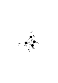
Figure 1: CoO₄ tetrahedron

It is convenient to choose the zero of energy from the condition Tr$V_{m,m\prime}=5\sum_{i}b_{0}(R_{i})=0$. The term $\hat{H}_{CF}$ in Eq. (13) may be split into cubic and trigonal parts:

$$\hat{H}_{CF}=\hat{H}_{cub}+\hat{H}_{trig}\ ,$$ (30)

since the ideal tetrahedron with $\frac{c}{a}=\sqrt{\frac{8}{3}}$ and $\delta=0$ is identical to cubic symmetry. In reality, however, $\frac{c}{a}$ deviates from the ideal value and $\delta\neq 0$. The trigonal field is described by three parameters. There exist several different systems of notation in the literature and we will use here the parameters $\Delta$, $\upsilon$, and $\upsilon^{\prime}$ like Koidl Koidl and MacFarlane MacFarlane (see also Ref. Bates, ). They are defined as a parametrization of the crystal field matrix elements $V_{mm^{\prime}}$ (Eq. (13)) in the one-particle basis of the trigonal coordinate system (the $z$ axis is the threefold axis pointing towards O₄):

$$\begin{array}[]{ll}|x\rangle=\sqrt{\frac{2}{3}}|x^{2}-y^{2}\rangle-\sqrt{\frac{1}{3}}|zx\rangle\\ |y\rangle=-\sqrt{\frac{2}{3}}|xy\rangle-\sqrt{\frac{1}{3}}|zy\rangle\\ |z\rangle=|z^{2}\rangle\\ |v\rangle=\sqrt{\frac{1}{3}}|x^{2}-y^{2}\rangle+\sqrt{\frac{2}{3}}|zx\rangle\\ |w\rangle=-\sqrt{\frac{1}{3}}|xy\rangle+\sqrt{\frac{2}{3}}|zy\rangle\ ,\\ \end{array}$$ (31)

where we have the usual real $d$-basis functions constructed out of the complex basis functions $|l\rangle=d^{+}_{l\sigma}|0\rangle$ on the right hand side. The three basis functions $|x\rangle$, $|y\rangle$ and $|z\rangle$ build up the $t_{2g}$ representation of the cubic group and $|v\rangle$, $|w\rangle$ span up the $e_{g}$ subspace. The one-particle crystal field matrix elements are given in this basis by:

$$\begin{array}[]{ll}V_{zz}=\frac{2}{5}\Delta-\frac{2\upsilon}{3}\\ V_{xx}=V_{yy}=\frac{2}{5}\Delta+\frac{\upsilon}{3}\\ V_{vv}=V_{ww}=-\frac{3}{5}\Delta\\ V_{xv}=\upsilon^{\prime}\;.\end{array}$$ (32)

The relationship between the $\Delta$, $\upsilon$, and $\upsilon^{\prime}$ parameters with the Stevens equivalent operators and other parametrizations used in the literature can be found in the Appendix.

If we substitute the ligand coordinates from Table 1 into $V_{mm\prime}$ in Eq. (14) and then transform them into the trigonal crystal field parameters we obtain

$$\Delta = -\frac{5}{27}\left\{b_{4}(R_{1})\frac{72(z_{1}^{2}a^{2}-z_{1}^{4})-3a^{4}+20\sqrt{6}z_{1}a^{3}}{24R_{1}^{4}}-b_{4}(R_{4})\right\},$$

$$\upsilon = \frac{b_{4}(R_{1})}{9R_{1}^{4}}\left\{\frac{20}{7}\left[3(z_{1}^{2}a^{2}-z_{1}^{4})-\frac{a^{4}}{8}\right]-\frac{5\sqrt{6}z_{1}a^{3}}{6}\right\}-\frac{20}{63}b_{4}(R_{4})$$ (33)

$$-\frac{3}{14}\left[b_{2}(R_{1})\frac{6z_{1}^{2}-a^{2}}{R_{1}^{2}}+2b_{2}(R_{4})\right],$$

$$\upsilon\prime = \frac{5b_{4}(R_{1})}{9R_{1}^{4}}\left\{\frac{\sqrt{2}}{7}\left[3(z_{1}^{2}a^{2}-z_{1}^{4})-\frac{a^{4}}{8}\right]-\frac{\sqrt{3}z_{1}a^{3}}{12}\right\}-\frac{\sqrt{2}}{9}b_{4}(R_{4})$$

$$+\frac{\sqrt{2}}{14}\left[b_{2}(R_{1})\frac{6z_{1}^{2}-a^{2}}{R_{1}^{2}}+2b_{2}(R_{4})\right],$$

where $z_{i}$ is the $z$ coordinate of the ligand O_i; $R_{1}=\sqrt{a^{2}/3+z_{1}^{2}},\ R_{4}=z_{4}$ are the corresponding distances.

The importance of the non-diagonal matrix element between $e_{g}$ and $t_{2g}$ states, $\upsilon^{\prime}$, was first pointed out in Refs. MacFarlane, and MacFarlane67, and will be outlined in the following, but it was not thoroughly treated in the standard text books. abragam Hopping integrals $t_{pdm}$ have been calculated from Harrison’s table. Harrison Then all the CF parameters depend only on one value: $\Delta_{pd}$. Its determination is complicated by the fact that the Coulomb repulsion $A_{d}$ is partially screened in semiconductors and it differs much more from free ion value than $B$ and $C$. That is the reason why we have used $\Delta_{pd}$ as an adjustable parameter. After determination of its value from experimental knowledge of cubic parameter $\Delta$, the other parameters $\upsilon$ and $\upsilon^{\prime}$, are determined by geometry.

For the spin-orbit and Zeeman terms we have

$$\hat{H}_{SO} = \frac{\xi_{d}}{2}\sum_{m,m\prime,s,s\prime}d_{m,s}^{{\dagger}}\mbox{\boldmath$L$}_{m,m\prime}\ \mbox{\boldmath$\sigma$}_{s,s\prime}\ d_{m\prime,s\prime}$$ (34)

$$\hat{H}_{Z} = \mu_{B}\left(g_{s}\hat{\bf S}+k\hat{\bf L}\right){\bf B}\ ,$$ (35)

here $\xi_{d}$ is the renormalized spin-orbit coupling, and $k$ is approximately given by Eq. (26); $\hat{\bf S}$ and $\hat{\bf L}$ are respectively the total spin and orbital angular momentum operators. Within the ${}^{4}F$ term, $H_{SO}$ may be rewritten as

$$\hat{H}_{SO,^{4}F}=\lambda\hat{\bf S}\hat{\bf L}\ ,\ \ {\rm with}\ \ \lambda=-\xi_{d}/3\ .$$ (36)

IV Spin Hamiltonian for the ground state manifold

As it was already noted in the Introduction, this second step of our calculation can be performed exactly by numerical diagonalization of the effective single-ion Hamiltonian (29) once we have determined all its parameters (see Appendix). In that sense it is not restricted to the ’weak’ field case. In addition to the numerical diagonalization, we derive below an analytic perturbative formula which is valid in the ’weak’ field case of ZnO:Co.

IV.1 Many-body basis

For a while let us neglect the spin-orbit coupling. Then the total spin $S$ and total angular momentum $L$ are conserved, because Coulomb interaction is rotationally invariant and does not depend on spin. The ground state for seven $d$-electrons (three holes) is $\left|{}^{4}F\right\rangle$ with $L=3,\ S=3/2$ and it is $(2L+1)(2S+1)=28$-fold degenerate. The eigenfunctions are $\left|L,M,m_{s}\right\rangle$, $M$ being the momentum projection on $z$ axis, $m_{s}$ the total spin projection. For $M=3$ and $m_{s}=\frac{3}{2}$ we have

$$\left|3,3,\frac{3}{2}\right\rangle=d_{0\uparrow}^{\dagger}d_{1\uparrow}^{\dagger}d_{2\uparrow}^{\dagger}\left|vac\right\rangle.$$

Acting on this state by $\hat{L}_{-}$ operator we obtain successively

$$\left|3,2,\frac{3}{2}\right\rangle=d_{-1\uparrow}^{\dagger}d_{1\uparrow}^{\dagger}d_{2\uparrow}^{\dagger}\left|vac\right\rangle,$$

$$\left|3,1,\frac{3}{2}\right\rangle=\left(\sqrt{\frac{2}{5}}d_{-2\uparrow}^{\dagger}d_{1\uparrow}^{\dagger}d_{2\uparrow}^{\dagger}+\sqrt{\frac{3}{5}}d_{-1\uparrow}^{\dagger}d_{0\uparrow}^{\dagger}d_{2\uparrow}^{\dagger}\right)\left|vac\right\rangle,$$

$$\left|3,0,\frac{3}{2}\right\rangle=\sqrt{\frac{1}{5}}\left(2d_{-2\uparrow}^{\dagger}d_{0\uparrow}^{\dagger}d_{2\uparrow}^{\dagger}+d_{-1\uparrow}^{\dagger}d_{0\uparrow}^{\dagger}d_{1\uparrow}^{\dagger}\right)\left|vac\right\rangle,\ etc.$$

Under the action of cubic crystal field this level splits into 1 singlet and 2 triplets. Then the basis functions may be labeled as $\left|3,\chi,\tilde{m},m_{s}\right\rangle$, where $\chi=A_{2},T_{2},T_{1}$ denotes the representation of the cubic group, $\tilde{m}$ is the projection of a fictive angular momentum within each manifold. We have

$$\left|3,A_{2},0,m_{s}\right\rangle = -\frac{\sqrt{5}}{3}\left|3,0,m_{s}\right\rangle+\frac{\sqrt{2}}{3}\left(\left|3,3,m_{s}\right\rangle-\left|3,-3,m_{s}\right\rangle\right)$$

$$\left|3,T_{2},\pm 1,m_{s}\right\rangle = \frac{1}{\sqrt{6}}\left|3,\mp 2,m_{s}\right\rangle\pm\sqrt{\frac{5}{6}}\left|3,\pm 1,m_{s}\right\rangle$$

$$\left|3,T_{2},0,m_{s}\right\rangle = \frac{1}{\sqrt{2}}\left(\left|3,3,m_{s}\right\rangle+\left|3,-3,m_{s}\right\rangle\right)$$ (37)

$$\left|3,T_{1},\pm 1,m_{s}\right\rangle = \mp\sqrt{\frac{5}{6}}\left|3,\mp 2,m_{s}\right\rangle+\frac{1}{\sqrt{6}}\left|3,\pm 1,m_{s}\right\rangle$$

$$\left|3,T_{1},0,m_{s}\right\rangle = -\frac{2}{3}\left|3,0,m_{s}\right\rangle-\frac{1}{3}\sqrt{\frac{5}{2}}\left(\left|3,3,m_{s}\right\rangle-\left|3,-3,m_{s}\right\rangle\right)\ .$$

The trigonal field splits the triplets into doublets and singlets and also couples the states of different manifolds with equal $\tilde{m}$. This is schematically shown in Fig. 2. The lowest excited level is ${}^{4}P$ with $L=1,\ S=3/2$

$$\left|1,1,\frac{3}{2}\right\rangle=\left(\sqrt{\frac{3}{5}}d_{-2\uparrow}^{\dagger}d_{1\uparrow}^{\dagger}d_{2\uparrow}^{\dagger}-\sqrt{\frac{2}{5}}d_{-1\uparrow}^{\dagger}d_{0\uparrow}^{\dagger}d_{2\uparrow}^{\dagger}\right)\left|vac\right\rangle,$$

$$\left|1,0,\frac{3}{2}\right\rangle=\sqrt{\frac{1}{5}}\left(d_{-2\uparrow}^{\dagger}d_{0\uparrow}^{\dagger}d_{2\uparrow}^{\dagger}-2d_{-1\uparrow}^{\dagger}d_{0\uparrow}^{\dagger}d_{1\uparrow}^{\dagger}\right)\left|vac\right\rangle,\ etc.$$

In the free ion it is separated by energy $15B$ from the ground state. The cubic field couples the states $\left|1,M,m_{s}\right\rangle$ and $\left|3,T_{1},\tilde{m},m_{s}\right\rangle$ with $\tilde{m}=M$. The trigonal field has also matrix elements between $\left|3,A_{2},\tilde{m},m_{s}\right\rangle$, $\left|3,T_{2},\tilde{m},m_{s}\right\rangle$ and $\left|1,\tilde{m},m_{s}\right\rangle$ states that are proportional to $v$ and $v^{\prime}$, thus they are much smaller.

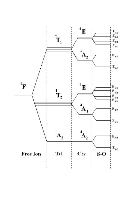
Figure 2: Qualitative splitting due to the cubic field, followed by the trigonal crystal field and by the SO effect.

IV.2 Perturbation theory

From the parameter values discussed below, it will become clear that we are in the regime where $15B\gg\Delta\gg\upsilon,\upsilon^{\prime},\lambda$. In the strong cubic crystal field case (i.e. when $\Delta\gg 15B$) a perturbative formula for zero field splitting $2D$ and the gyromagnetic factors $g_{\parallel}$ and $g_{\perp}$ was developed by MacFarlane.MacFarlane67 ; MacFarlane But it is not adequate in the present situation. Now, we can define four small values $\frac{\Delta}{(15B)}$, $\frac{\upsilon}{\Delta}\sim\frac{\upsilon^{\prime}}{\Delta}\sim\frac{\lambda}{\Delta}$. In fact, we have $15B\gg\Delta$, and the value $\Delta/15B$ being almost of the same order of magnitude as $v/\Delta$, then the ratio

$$\frac{v}{15B}=\frac{v}{\Delta}\frac{\Delta}{15B}$$

can be considered as an order of magnitude smaller than $\Delta/15B$. This justifies the application of the weak crystal field approach.

We will proceed in three steps that may be regarded as three subsequent canonical transformations of our Hamiltonian similar to Eq. (4). First, we eliminate the coupling with ${}^{4}P$ states retaining only the order $\Delta/15B$ (the explicit use of weak CF scheme). Then only the states $\left|3,T_{1},\tilde{m},m_{s}\right\rangle$ acquire an admixture

$$\left|T_{1},\tilde{m},m_{s}\right\rangle=\left|3,T_{1},\tilde{m},m_{s}\right\rangle+\frac{\left\langle 1,\tilde{m},m_{s}\right|\hat{H}_{CF}\left|3,T_{1},\tilde{m},m_{s}\right\rangle}{\left(E_{T_{1}0}-E_{P0}\right)}\left|1,\tilde{m},m_{s}\right\rangle\ ,$$ (38)

where

$$\frac{\left\langle 1,\tilde{m},m_{s}\right|\hat{H}_{CF}\left|3,T_{1},\tilde{m},m_{s}\right\rangle}{\left(E_{T_{1}0}-E_{P0}\right)}\simeq\frac{2}{5}\frac{\Delta}{15B}\equiv\kappa_{P}\ .$$

We thus obtain an effective Hamiltonian acting in the ${}^{4}F$ subspace. In the next step we consider the perturbation due to the trigonal field with the small parameters $\frac{\upsilon}{\Delta}$ and $\frac{\upsilon^{\prime}}{\Delta}$. In the following we will use the first order ground state wave function of the approximately diagonal crystal field Hamiltonian,exactCF i.e.

$$\left|\psi_{0}\right\rangle=\left|A_{2},0,m_{s}\right\rangle\approx\left|3,A_{2},0,m_{s}\right\rangle-\kappa_{0}\left|T_{1},0,m_{s}\right\rangle\,,$$

as well as the excited states

$$\left|T_{2},0,m_{s}\right\rangle \approx \left|3,T_{2},0,m_{s}\right\rangle$$

$$\left|T_{2},\pm 1,m_{s}\right\rangle \approx \left|3,T_{2},\pm 1,m_{s}\right\rangle\mp\kappa_{2}\left|T_{1},\pm 1,m_{s}\right\rangle$$ (39)

$$\left|T_{1},0,m_{s}\right\rangle_{t} \approx \left|T_{1},0,m_{s}\right\rangle+\kappa_{0}\left|3,A_{2},0,m_{s}\right\rangle$$

$$\left|T_{1},\pm 1,m_{s}\right\rangle_{t} \approx \left|T_{1},\pm 1,m_{s}\right\rangle\pm\kappa_{2}\left|3,T_{2},\pm 1,m_{s}\right\rangle\ ,$$

where

$$\kappa_{0}\equiv\frac{\upsilon^{\prime}\sqrt{10}}{5\left(E_{T_{1}0}-E_{A_{2}}\right)}\left(1+2\kappa_{P}\right)\simeq\frac{\upsilon^{\prime}\sqrt{10}}{9\Delta}\left(1+2\kappa_{P}\right)\ ,$$

$$\kappa_{2}\equiv\frac{\upsilon+2\upsilon^{\prime}\sqrt{2}}{2\sqrt{5}\left(E_{T_{1}1}-E_{T_{2}1}\right)}+\frac{\kappa_{P}}{\sqrt{5}\left(E_{T_{1}1}-E_{T_{2}1}\right)}\left(\upsilon-\frac{3\sqrt{2}}{2}\upsilon^{\prime}\right)\ .$$

The corresponding energies are

$$E_{A_{2}} \approx -\frac{6\Delta}{5}$$

$$E_{T_{2}0} \approx -\frac{\Delta}{5}+\frac{\upsilon}{3}$$

$$E_{T_{2}1} \approx -\frac{\Delta}{5}-\frac{\upsilon}{6}$$ (40)

$$E_{T_{1}0} \approx \frac{3\Delta}{5}+\frac{3\upsilon}{5}+\frac{4\upsilon^{\prime}\sqrt{2}}{5}-\frac{4}{5}\frac{\Delta^{2}}{75B}$$

$$E_{T_{1}1} \approx \frac{3\Delta}{5}-\frac{3\upsilon}{10}+\frac{\upsilon^{\prime}\sqrt{2}}{210}-\frac{4}{5}\frac{\Delta^{2}}{75B}\ .$$

Then we consider the spin-orbit interaction as a perturbation with respect to the crystal field Hamiltonian. We thus obtain the usual formulae for the $g$-factor and the anisotropy $D$

$$g_{\mu\nu}-g_{s}=-2\lambda k\Lambda_{\mu\nu}\ ,$$ (41)

$$D=-\lambda^{2}\left(\Lambda_{zz}-\Lambda_{xx}\right)\ ,$$ (42)

where

$$\Lambda_{\mu\nu}=\sum_{n\neq 0}\frac{\left\langle\psi_{0}\right|\hat{L}^{\mu}\left|n\right\rangle\left\langle n\right|\hat{L}^{\nu}\left|\psi_{0}\right\rangle}{E_{n}-E_{0}}\ ,$$ (43)

with $E_{0}=E_{A_{2}}$ and $\lambda$ is defined in Eq. (36). These are the parameters appearing in the effective spin $(S=\frac{3}{2})$ Hamiltonian:

$$H_{spin}=\mu_{B}g_{\parallel}B_{z}S_{z}+\mu_{B}g_{\perp}\left(B_{x}S_{x}+B_{y}S_{y}\right)+D\left[S_{z}^{2}-\frac{1}{3}S\left(S+1\right)\right].$$ (44)

Let us note that all energy denominators appearing in $\Lambda_{\mu\nu}$ (43) are of the order of cubic splitting $\Delta$. Thus, the perturbation theory requires the SO coupling to fulfill $\lambda\ll\Delta$. But $\lambda$ may be of the same order of magnitude as $\upsilon$ and $\upsilon^{\prime}$. The operator $\hat{L}_{z}$ couples the ground state only with $\left|T_{2},0,m_{s}\right\rangle$

$$\hat{L}_{z}\left|A_{2},0,m_{s}\right\rangle=\left(2+\kappa_{0}\sqrt{5}\right)\left|T_{2},0,m_{s}\right\rangle\ ,$$

then

$$\Lambda_{zz}=\frac{4\left(1+\kappa_{0}\sqrt{5}\right)}{\left(E_{T_{2}0}-E_{A_{2}}\right)}\ .$$

For $\hat{L}_{x}=(\hat{L}_{+}+\hat{L}_{-})/2$ we have

$$\hat{L}_{x}\left|A_{2},0,m_{s}\right\rangle=\frac{1}{2}\left\{-2\sqrt{2}\left(\left|T_{2},1,m_{s}\right\rangle-\left|T_{2},-1,m_{s}\right\rangle\right)\right.$$

$$-\kappa_{0}\left.\left[-\frac{3\sqrt{2}}{2}\left(\left|T_{1},1,m_{s}\right\rangle+\left|T_{1},-1,m_{s}\right\rangle\right)-\sqrt{\frac{5}{2}}\left(\left|T_{2},1,m_{s}\right\rangle-\left|T_{2},-1,m_{s}\right\rangle\right)\right]\right\}\;,$$

and

$$\Lambda_{xx}\simeq\frac{4\left(1-\frac{\kappa_{0}\sqrt{5}}{2}\right)}{\left(E_{T_{2}1}-E_{A_{2}}\right)}\ .$$

The anisotropy constant appears only in the third order (second order of spin-orbit and first order of trigonal field)

$$D\approx\frac{4\lambda^{2}}{\Delta}\left(\frac{\upsilon}{2\Delta}-\frac{3\kappa_{0}\sqrt{5}}{4}\right)\approx\frac{\lambda^{2}}{\Delta}\left[2\frac{\upsilon}{\Delta}-\frac{10\sqrt{2}}{3}\frac{v^{\prime}}{\Delta}\left(1+2\kappa_{P}\right)\right].$$

The final results are:

$$\begin{array}[]{ll}D=\frac{\lambda^{2}}{\Delta}\left[2\frac{\upsilon}{\Delta}-\frac{10\sqrt{2}}{3}\frac{\upsilon^{\prime}}{\Delta}\left(1+\frac{4}{75}\frac{\Delta}{B}\right)\right]&\\ g_{\parallel}=g_{s}-\frac{8\lambda}{\Delta}k\left[1-\frac{\upsilon}{3\Delta}+\frac{5\sqrt{2}}{9\Delta}\upsilon^{\prime}\left(1+\frac{4}{75}\frac{\Delta}{B}\right)\right]&\\ g_{\perp}=g_{s}-\frac{8\lambda}{\Delta}k\left[1+\frac{\upsilon}{6\Delta}-\frac{5\sqrt{2}}{18\Delta}\upsilon^{\prime}\left(1+\frac{4}{75}\frac{\Delta}{B}\right)\right]\ .&\end{array}$$ (45)

An alternative perturbative formula for zero-field splitting $2D$, which is valid in the present situation, was derived by Mao-Lu and Min-Guang.mao However, our result is much more compact than theirs (the Eqs. (5)-(9) of Ref. mao, take one page and a half) and, correspondingly, more practicable. We have checked that the difference between the compact formulas (45) and the result given in Ref. mao, is very small and can be neglected in numerical applications.

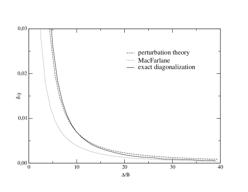
Figure 3: Comparison between our perturbation theory (45) for the weak field case (dashed line), the result derived by MacFarlane MacFarlane in the strong field case (dotted),and the exact diagonalization calculation for $\delta g=g_{\perp}-g_{\parallel}$ (full line).

To check the applicability of our perturbation theory (45) we compared it with the exact diagonalization (see Appendix). We fixed the parameters (in inverse centimeters) $\upsilon=54$, $\upsilon^{\prime}=-213$, $C=3148$, $B=804$, $k=0.85$, and $k\xi_{d,0}=481$ to those values which we derived for Co²⁺ in ZnO (see next Section) and varied $\Delta/B$ to display the different regimes. As one can see from Fig. 3, the difference of $g$-factors $\delta g=g_{\perp}-g_{\parallel}$ from our formula compares well with the exact diagonalization for $\Delta/B$ up to 15. Therefore, we can certainly apply it to the case of Co²⁺ in ZnO where $\Delta/B$ is roughly 5 and where there are considerable deviations for MacFarlanes formula. MacFarlane On the other hand, the exact diagonalization converges towards MacFarlanes formula for large values of $\Delta/B$.

V Application to ZnO:Co

We apply our theory to the calculation of spin-Hamiltonian parameters for Co impurity in zinc oxide. As input, we need the following parameters of $\hat{H}$ (Eq. (1)): (i) the structure of the Co environment given in Table 1, (ii) the charge transfer energy $\Delta_{pd}$ (Eq. (18)), (iii) the free-ion spin-orbit coupling $\xi_{d,0}\approx 567\ {\rm cm}^{-1}$ (see e.g. Table 7.6 of Ref. abragam, ), (iv) the Racah’s parameters $B_{0}\approx 1115\ {\rm cm}^{-1}$ and $C_{0}\approx 4366\ {\rm cm}^{-1}$ (from Table 7.5 of Ref. abragam, ).

As was mentioned above, we calculate the hopping integrals that enter $\hat{H}$ (Eqs. (1) and (3)) from Harrison’s expressionsHarrison

$$t_{pdm}(R)=\eta_{pdm}\frac{\hbar^{2}r_{d}^{3/2}}{mR^{7/2}},\ \eta_{pd\sigma}=-2.95,\ \eta_{pd\pi}=1.36,$$ (46)

where the value $r_{d}=0.76\ \mathrm{\AA}$ for Co ion. The distance $R$ is measured in Å and $t_{pdm}$ in eV (1 eV = 8065.5 cm^-1). This gives, e.g. for $t_{pd\sigma}(R_{4})\approx 1.34\ \mathrm{eV}$. The coefficients $b_{k}$ (Eq. (15)) are inversely proportional to the charge transfer energy $\Delta_{pd}$. We choose the $\Delta_{pd}\approx 3.6\ {\rm eV}\approx 28800\ {\rm cm}^{-1}$ so that the cubic splitting $\Delta$ (Eq. (33)) is equal to the experimentally determined valueKoidl $\Delta=4070$ cm^-1. Then, the trigonal CF parameters $\upsilon\approx 54\ {\rm cm}^{-1}$ and $\upsilon^{\prime}\approx-213\ {\rm cm}^{-1}$ are unambiguously determined by the Co environment via Eqs. (33) and are not additionally adjusted. The SO and angular momentum reduction factor $k\approx 0.85$ was calculated from Eq. (26). This gives the spin orbit coupling $\xi_{d}=k\xi_{d,0}\approx 481\ {\rm cm}^{-1},\ \lambda=-\xi_{d}/3\approx-160\ {\rm cm}^{-1}$ very close to the values met in the literature (and adjusted empirically): $\xi_{d}=450\ {\rm cm}^{-1}$ in Ref. MacFarlane, , and $\xi_{d}=430\ {\rm cm}^{-1}$ in Ref. Koidl, . From our above consideration, we have seen that the reduction factors for Coulomb interaction may differ from those of SO and angular momentum terms. Nevertheless, an order of magnitude estimate may be done as $B\approx k^{2}B_{0}\approx 804\ {\rm cm}^{-1}$ and $C\approx k^{2}C_{0}\approx 3148\ {\rm cm}^{-1}$. We adopt these values for our calculations. The agreement with the experimentally adjusted values $B=750$ cm^-1, $C=3500$ cm^-1 of MacFarlaneMacFarlane is very good, keeping in mind the roughness of the estimate. We should also note that the influence of the $B$ and $C$ parameters on the calculated $g$-factors and the zero field splitting $2D$ is rather small. So, using instead of our estimations for $B$ and $C$ the values of MacFarlane (and keeping all the other parameters constant) leads to $2D=4.882$, $g_{\parallel}=2.230$, and $g_{\perp}=2.256$, quite close to the results listed in Table II.

The parameters of the ground state spin-Hamiltonian (Eq. (44)) obtained by exact diagonalization of single-ion Hamiltonian $\hat{H}_{eff}$ (Eq. (29)) are shown in the Table 2. Note that our sign convention for the crystal field parameters corresponds to the electron representation in contrast to the hole representation used in Refs. Koidl, and MacFarlane, . The agreement with purely empirical approaches, where all parameters are fitted to experiment, is very good. We show also the parameters for the excited state.

	P. KoidlKoidl	R.M. MacFarlaneMacFarlane	Present work	experiment
$\upsilon$	-120	-400	54
$\upsilon^{\prime}$	-320	-350	-213
$\Delta$	4000	4000	4070	4070Koidl
$B$	760	750	804
$C$	3500	3500	3148
$k$	1	0.8	0.85
$k\xi_{d,0}$	430	450	481
$2D$	5.44	5.41	4.91	5.52Sati05
$g_{\parallel}$	2.24	2.20	2.23	2.236Sati05
$g_{\perp}$	2.28	2.23	2.26	2.277Sati05
$2D^{\prime}$	21.4	90.3	5.8	38Koidl
$g_{\parallel}^{\prime}$	2.85	3.36	4.22	3.52Ferrand
$E_{{}^{2}E\bar{E}}-E_{{}^{4}A\bar{E}}$	15171	15050	14381	15123Ferrand

Table 2: Measured ESRSati05 and magneto-opticFerrand data, compared to those calculated from CF theory with empirical parametersKoidl ; MacFarlane or estimated from our approach. $2D\ (2D^{\prime})$ and $g\ (g^{\prime})$ are the values for the ground (excited) state. The energy unit is inverse centimeter. In the empirical CF theory Koidl ; MacFarlane all the 7 parameters listed in the upper part of the table are used as fitting parameters, whereas they are microscopically calculated in our approach fixing only the cubic CF splitting $\Delta$ to the experimental value.

Table 3 compares the spin-Hamiltonian parameters obtained by analytic perturbative approach (Eqs. (45)) with the results of the exact diagonalization and experiment. We see that the analytic results lie within 15% of accuracy. For the phenomenological parameter set of KoidlKoidl the accuracy is about 20%.Sati05 The reason is that in our set the absolute values of trigonal parameters are smaller than for the set of Ref. Koidl, and the cubic splitting is the same, thus the perturbation theory for our set converges better. The main reason of the deviation from exact diagonalization is our neglect of the interaction with ${}^{2}G$ term that violates the Hund’s rule, but nevertheless lies rather low in energy, just above the ${}^{4}P$ term (see Table 4). This deviation is remarkable for $2D$, but much less for the $g$-factors.

	experiment	diagonalization	perturbation theory
$2D$	5.52	4.91	4.31
$g_{\parallel}$	2.24	2.23	2.25
$g_{\perp}$	2.28	2.26	2.28

Table 3: ESR data as calculated from the numerical diagonalization and the perturbation theory using the calculated crystal field parameters.

VI Conclusion

We have shown that Harrison’s parametrization of electronic structure of solidsHarrison may be successfully applied to the calculation of spin-Hamiltonian parameters (Eq. (44)) for TMI impurities in semiconductors (Eq. (45)). It is especially useful for the description of low symmetry paramagnetic centers as it provides the connection between CF parameters and the geometry of TMI surroundings (Eq. (33)). Thus, the number of empirically adjustable parameters is substantially reduced.

We have demonstrated that the physical reason for the possibility to apply the CF concept to TMI in semiconductors is the strong Coulomb repulsion within the $d$-shell. It provides the large value of charge transfer energy $\Delta_{pd}$ (Eqs. (6) and (18)) even in the case when the mean-field energy of the $d$-level falls into the valence band. We have given the explicit form of the canonical transformation (Eqs. (4) and (5)) of the many-body Hamiltonian (Eq.(1)) and basis functions, which exploits this strongly correlated feature of the TMI subsystem (Eq. (11)), and provides the effective single-ion Hamiltonian (Eq. (II.1)). The latter connects the CF Hamiltonian with the geometry of local surroundings of the impurity and with the parameters of the electronic structure (Eqs. (13) to (15)). The transformation (Eqs. (4) and (5)) accounts for the covalency in the ’weak’ CF case within the Heitler-London configuration interaction approach. When applied to the spin-orbit, Zeeman and Coulomb terms, it renormalizes their parameters by covalency.

We have applied this theory to the Co impurity in ZnO. We have adjusted only one parameter of our starting $p$-$d$ Hamiltonian (Eq. (1)), which acts in an energy scale of several eV. In the result, we have fairly well reproduced a number of measurable quantities available from ESR and optical experiments. Note that these values reflect the tiny features of electronic structure (magnetic anisotropy, Zeeman splitting), which have the scale of several cm^-1. The results indicate that the proposed theory catches the essential physics of TMI in semiconductors.

Appendix: Exact diagonalization for $3d^{3}$ ($3d^{7}$)

In this section we detail the numerical calculations of the exact diagonalization for 3 particles on a $3d$-level. The case of interest namely $3d^{7}$ can be obtained from the former using a particle-hole transformation.

The number of states for 3 particles on a $d$ level is $10\times 9\times 8/3!=120$. These states can be labelled by usual quantum numbers for total spin and angular momentum, we thus obtain different multiplets: ${}^{4}F$ for which $S=\frac{3}{2}$, $L=3$, this multiplet contains $(2S+1)(2L+1)=28$ different states. We also have ${}^{4}P$ $(S=\frac{3}{2},L=1)$, ${}^{2}H$ $(S=\frac{1}{2},L=5)$, ${}^{2}G$ $(S=\frac{1}{2},L=4)$, ${}^{2}F$ $(S=\frac{1}{2},L=3)$, ${}^{2}D$ and ${}^{2}D^{\prime}$ $(S=\frac{1}{2},L=2)$, and finally ${}^{2}P$ $(S=\frac{1}{2},L=1)$. This basis will be noted $\{|\alpha\rangle=|S,L,M,m_{s},\epsilon\rangle\}$, the last quantum number $\epsilon$ is needed to distinguish states belonging to the 2 multiplets ${}^{2}D$ and ${}^{2}D^{\prime}$.

The $\{|\alpha\rangle\}$ basis is the natural one for the Coulomb interaction as well as the Zeeman Hamiltonian, however an other basis emerges when writing the one-body part of the Hamiltonian, namely the crystal-field and spin-orbit terms. Let us denote by $\{|i\rangle,i=1..10\}$, the basis for one electron on a $d$ level. $i$ is an index for the $(m_{l},\sigma)$ state, where $m_{l}$ and $\sigma$ are the momentum and spin quantum numbers. We can construct a new basis of 120 states $\{|n\rangle\ =\ |ijk\rangle\ =\ c^{{\dagger}}_{i}c^{{\dagger}}_{j}c^{{\dagger}}_{k}|\ vac\rangle,\ \ i<j<k:1..10,\ \ n:1..120\}$ where $|\ vac\rangle$ is the empty $d$ level.

The complete Hamiltonian has been written in Eq. (29). The Coulomb part is diagonal in the $\{|\alpha\rangle\}$ basis, and the Tab. 4 gives the different energy values.

Term	Coulomb energy
${}^{4}F$	$3A-15B$
${}^{4}P$	$3A$
${}^{2}G$	$3A-11B+3C$
${}^{2}H$	$3A-6B+3C$
${}^{2}P$	$3A-6B+3C$
${}^{2}F$	$3A+9B+3C$
${}^{2}D,\ ^{2}D^{\prime}$	$3A+5B+5C\pm\sqrt{(}193B^{2}+8BC+4C^{2})$

Table 4: Coulomb energy depending on the multiplet

Contrary to MacFarlane’s workMacFarlane where the Zeeman Hamiltonian is treated in a perturbative manner, it is here diagonalized on the same foot as the other terms. In the $\{|\alpha\rangle\}$ basis, the Zeeman Hamiltonian is block-diagonal, and the non zero matrix elements just connect states by $\hat{L}_{+(-)}$ or $\hat{S}_{+(-)}$. The crystal field Hamiltonian is the sum of the cubic and trigonal parts. The one particle matrix elements of $\hat{H}_{CF}$ (Eq. 13)) may also be expressed in terms of Stevens equivalent operators abragam

$$\hat{H}_{cub}=-\frac{2}{3}B^{0}_{4}(\hat{O}_{4}^{0}-20\sqrt{2}\hat{O}_{4}^{3})\quad\hat{H}_{trig}=B^{{}^{\prime}}_{2}\hat{O}_{2}^{0}+B_{4}^{{}^{\prime}}\hat{O}_{4}^{0}$$ (47)

corresponding to a $d^{1}$ configuration. The Stevens operators are given by

$$\hat{O}_{4}^{0} = 35\hat{L}_{z}^{4}-30L(L+1)\hat{L}_{z}^{2}+25\hat{L}_{z}^{2}-6L(L+1)+3L^{2}(L+1)^{2}$$

$$\hat{O}_{4}^{3} = \frac{1}{4}\{\hat{L}_{z}(\hat{L}_{+}^{3}+\hat{L}_{-}^{3})+(\hat{L}_{+}^{3}+\hat{L}_{-}^{3})\hat{L}_{z}\}$$ (48)

$$\hat{O}_{2}^{0} = 3\hat{L}_{z}^{2}-L(L+1)\ ,$$

where the operators $\hat{L}_{z}$,$\hat{L}_{+}$, or $\hat{L}_{-}$ are one particle operators.

In analytic calculations we have used the $\{|\alpha\rangle\}$ basis and for the $d^{7}$ configuration the crystal field Hamiltonians (Eq. (47)) have to be used with the parameters

$$\tilde{B}^{0}_{4}=-\frac{B^{0}_{4}}{5},\ \tilde{B}^{{}^{\prime}}_{4}=-\frac{B^{{}^{\prime}}_{4}}{5},\ \tilde{B}^{{}^{\prime}}_{2}=\frac{B^{{}^{\prime}}_{2}}{5}.$$ (49)

The parameters $\Delta$, $\upsilon$, and $\upsilon^{\prime}$, previously defined in Eq. (32), are connected with the Stevens parameters by:

$$\begin{array}[]{ll}B^{0}_{4}=-\frac{\Delta}{120}-\frac{1}{360}(\upsilon+\frac{3\sqrt{2}}{2}\upsilon^{\prime})&\\ B^{\prime}_{4}=-\frac{1}{140}(\upsilon+\frac{3\sqrt{2}}{2}\upsilon^{\prime})&\\ B^{\prime}_{2}=\frac{\upsilon-2\sqrt{2}\upsilon^{\prime}}{21}\;.&\end{array}$$ (50)

Using Eq. (33) we obtain

$$\tilde{B}_{4}^{0} = -\frac{\sqrt{6}}{2880}b_{4}(R_{1})\frac{z_{1}a^{3}}{R_{1}^{4}}$$

$$\tilde{B}_{4}^{\prime} = -\frac{1}{140}\left\{b_{4}(R_{1})\frac{7\sqrt{6}z_{1}a^{3}+72(z_{1}^{4}-z_{1}^{2}a^{2})+3a^{4}}{216R_{1}^{4}}+\frac{b_{4}(R_{4})}{9}\right\}$$ (51)

$$\tilde{B}_{2}^{\prime} = -\frac{1}{210}\left\{b_{2}(R_{1})\frac{6z_{1}^{2}-a^{2}}{R_{1}^{2}}+2b_{2}(R_{4})\right\},$$

where $z_{i}$ is the $z$ coordinate of the ligand O_i; $R_{1}=\sqrt{a^{2}/3+z_{1}^{2}},\ R_{4}=z_{4}$ are the corresponding distances. For completeness we give here also the relation with another parameter set, that is often met in the literature

$$Dq=12B^{0}_{4},\ D\tau=12B^{\prime}_{4},\ D\sigma=-3B^{\prime}_{2}.$$ (52)

This set is used e.g. in Ref. mao, .

The crystal field Hamiltonian is easily written in the one-particle basis $\{|i\rangle,i=1..10\}$, where one evaluates the matrix elements $H^{CF}_{ij}=\langle i|H_{CF}|j\rangle$. Then the matrix elements of the CF Hamiltonian can be written in the 3-particle basis $\{|n\rangle=|ijk\rangle\}$ as follows

$$\langle k^{\prime}j^{\prime}i^{\prime}|H_{CF}|ijk\rangle=H^{CF}_{i^{\prime}i}(\delta_{j^{\prime}j}\delta_{k^{\prime}k}-\delta_{j^{\prime}k}\delta_{k^{\prime}j})-H^{CF}_{i^{\prime}j}(\delta_{j^{\prime}i}\delta_{k^{\prime}k}-\delta_{j^{\prime}k}\delta_{k^{\prime}i})+H^{CF}_{i^{\prime}k}(\delta_{j^{\prime}i}\delta_{k^{\prime}j}-\delta_{j^{\prime}j}\delta_{k^{\prime}i})$$

$$-H^{CF}_{j^{\prime}i}(\delta_{i^{\prime}j}\delta_{k^{\prime}k}-\delta_{i^{\prime}k}\delta_{k^{\prime}j})+H^{CF}_{j^{\prime}j}(\delta_{i^{\prime}i}\delta_{k^{\prime}k}-\delta_{i^{\prime}k}\delta_{k^{\prime}i})-H^{CF}_{j^{\prime}k}(\delta_{i^{\prime}i}\delta_{k^{\prime}j}-\delta_{i^{\prime}j}\delta_{k^{\prime}i})$$

$$+H^{CF}_{k^{\prime}i}(\delta_{i^{\prime}j}\delta_{j^{\prime}k}-\delta_{i^{\prime}k}\delta_{j^{\prime}j})-H^{CF}_{k^{\prime}j}(\delta_{i^{\prime}i}\delta_{j^{\prime}k}-\delta_{i^{\prime}k}\delta_{j^{\prime}i})+H^{CF}_{k^{\prime}k}(\delta_{i^{\prime}i}\delta_{j^{\prime}j}-\delta_{i^{\prime}j}\delta_{j^{\prime}i})$$

where $\delta$ is the Kronecker symbol. The spin-orbit term (Eq. (34)) is also easily written in the one-particle basis $\{|i\rangle\}$, then in the 3-particle one $\{|ijk\rangle\}$, using the preceding expansion.

At this stage we have some part of the total Hamiltonian written in the $\{|\alpha\rangle\}$ basis, the other one in the $\{|ijk\rangle\}$ one. To perform the numerical diagonalization, the last quantity needed is the transformation matrix to connect these two basis. The transformation basis is a kind of Clebsh-Gordan coefficient matrix for three particles constrained by Pauli principle.

References

- (1) H.A. Weakliem, J. Chem. Phys. 36, 2117 (1962).
- (2) P. Koidl, Phys. Rev. B 15, 2493 (1977).
- (3) A. Abragam and B. Bleaney, Electron Paramagnetic Resonance of Transition Ions, Dover Publications (New York) 1986.
- (4) H. Bethe, Ann. Phys 3, 133 (1929); english translation in Selected Works of Hans A. Bethe, World Scientific (Singapore) 1997.
- (5) S. Sugano, Y. Tanabe, and H. Kamimura, Multiplets of Transition Metal Ions in Crystals, Academic (New York) 1970.
- (6) J.S. Griffith, The Theory of Transition Metal Ions, Cambridge University Press (London) 1971.
- (7) According another classification,Bethe ; abragam the ’weak’ field for 3 ions is called ’intermediate’ field, and ’weak’ field case concerns -ions, where cubic splitting is less than spin-orbit coupling.
- (8) M.D. Kuzmin, A.I. Popov, A.K. Zvezdin, phys. stat. sol. (b) 168, 201 (1991).
- (9) W.A. Harrison, Electronic structure and the Properties of Solids, Freeman (San Francisco) 1980.
- (10) T. Mizokawa and A. Fujimori, Phys. Rev. B 48, 14150 (1993); J.Dreyhsig, J. Phys. Chem. Sol. 59, 31 (1998).
- (11) P. Sati, R.Hayn, R. Kuzian, S. Régnier, S.Schäfer, A.Stepanov, C. Morhain, C. Deparis, M. Laügt, M. Goiran, Z. Golacki, Phys. Rev. Lett. 96, 017203 (2006).
- (12) R.M. MacFarlane, Phys. Rev. B 1, 989 (1970).
- (13) C.A. Bates and P.E. Chandler, J. Phys. C: Solid State Phys. 4, 2713 (1971).
- (14) Du Mao-Lu and Zhao Min-Guang, J. Phys. C: Solid State Phys. 21, 1561 (1988).
- (15) K. Koepernik and H. Eschrig, Phys. Rev. B 59, 1743 (1999).
- (16) A. Messiah, Quantum Mechanics, Dover Publications (New York) 1999.
- (17) M.I. Bradbury and D.J. Newman, Chem. Phys. Letters 1, 44 (1967). For review see D.J. Newman, and B. Ng, Rep. Prog. Phys. 52, 699 (1989)
- (18) A. Fazzio, M.J. Caldas, and A. Zunger, Phys. Rev. B 30, 3430 (1984)
- (19) T. M. Sabine and S. Hogg, Acta Cryst. B 25, 2254 (1969).
- (20) R.M. MacFarlane, J. Chem. Phys. 47, 2066 (1967).
- (21) In the subspace, the CF part of the Hamiltonian may be exactly solved analytically. Villeret90 Unfortunately, this is not the case for the spin-orbit interaction matrix. As the SO coupling strength in the subspace , we restrict our consideration to the lowest order of perturbation theory.
- (22) M. Villeret, S. Rodriguez, and E. Kartheuser, J. Appl. Phys. 67, 4221 (1990)
- (23) W. Pacuski, D. Ferrand, J. Cibert, C. Deparis, J. A. Gaj, P. Kossacki, C. Morhain, Phys. Rev. B 73, 035214 (2006).