Test of Local Scale Invariance from the direct measurement of the response function in the Ising model quenched to and to below $T_{C}$

Abstract

In order to check on a recent suggestion that local scale invariance [M.Henkel et al. Phys.Rev.Lett. 87, 265701 (2001)] might hold when the dynamics is of Gaussian nature, we have carried out the measurement of the response function in the kinetic Ising model with Glauber dynamics quenched to $T_{C}$ in $d=4$, where Gaussian behavior is expected to apply, and in the two other cases of the $d=2$ model quenched to $T_{C}$ and to below $T_{C}$, where instead deviations from Gaussian behavior are expected to appear. We find that in the $d=4$ case there is an excellent agreement between the numerical data, the local scale invariance prediction and the analytical Gaussian approximation. No logarithmic corrections are numerically detected. Conversely, in the $d=2$ cases, both in the quench to $T_{C}$ and to below $T_{C}$, sizable deviations of the local scale invariance behavior from the numerical data are observed. These results do support the idea that local scale invariance might miss to capture the non Gaussian features of the dynamics. The considerable precision needed for the comparison has been achieved through the use of a fast new algorithm for the measurement of the response function without applying the external field. From these high quality data we obtain $a=0.27\pm 0.002$ for the scaling exponent of the response function in the $d=2$ Ising model quenched to below $T_{C}$, in agreement with previous results.

PACS: 05.70.Ln, 75.40.Gb, 05.40.-a

I Introduction

The non equilibrium dynamics of aging and slowly evolving systems is a topic of current and wide interest Cugliandolo . Much work has been devoted to the understanding of two times quantities such as the auto-correlation function $C(t,s)=\langle\phi(\vec{x},t)\phi(\vec{x},s)\rangle$ and the auto-response function $R(t,s)=\delta\langle\phi(\vec{x},t)\rangle/\delta h(\vec{x},s)$, where $\phi(\vec{x},t)$ is the order parameter at the space-time point $(\vec{x},t)$, $h(\vec{x},t)$ is the conjugate external field and the averages are taken over the thermal noise and the initial condition with $t\geq s$. The interest in the relation between these two quantities dates back to the solution by Cugliandolo and KurchanCuglia2 of the $p$-spin spherical model, where they introduced the fluctuation-dissipation relation as a measure of the distance from equilibrium. Furthermore, this relation can encode important information on the structure of the equilibrium state Cuglia3 .

One among the simplest examples of systems exhibiting aging and slow dynamics is a ferromagnetic model evolving with a dissipative dynamics after a quench from an infinite temperature to a final temperature $T$ smaller than or equal to the critical temperature $T_{C}$. In both cases, the slow relaxation entails the separation of the time scales. That is, when $s$ becomes large enough, the range of $\tau=t-s$ can be devided into the short $\tau\ll s$ and the long $\tau\gg s$ time separation, with quite different behaviors in the two regimes. The first one is the quasi-equilibrium or stationary regime, where the two time quantities are time translation invariant (TTI) and exhibit the same behavior as if equilibrium at the final temperature of the quench had been reached. The second one is a genuine off equilibrium regime, where aging becomes manifest. A crucial point is how these two behaviors are matched. The generic pattern for phase-ordering systems is that the matching is multiplicative in the quences to $T_{C}$ and additive in the quenches to below $T_{C}$. The first one is well documented by analytical calculations. For the second one, although the analytical evidence is less abundant, the additivity is required on general grounds by the weak ergodicity breaking scenario Cugliandolo .

To be more specific, in the case of the quench to $T_{C}$, using the methods of the field theoretical renormalization group (RG), the evolution equations for $C(t,s)$ and $R(t,s)$ are obtained by means of a series expansion around the Gaussian fixed point Schmit ; Cala1 ; Cala1b . The solution of these equations gives for $R(t,s)$ the scaling form

$$R(t,s)=s^{-(1+a)}F_{R}(t/s)$$ (1)

with the additional requirement that the scaling function must be of the form

$$F_{R}(x)=A_{R}(x-1)^{-(1+a)}x^{\theta}f_{R}(x)$$ (2)

where $a=(d-2+\eta)/z$, $d$ is the space dimensionality, $\eta$ and $z$ are the usual static and dynamic critical exponents, $\theta$ is the initial slip exponent and $\lim_{x\to\infty}f_{R}(x)=1$ Schmit ; Cala1 . A similar result is obtained for the correlation function Schmit ; Cala1 ; Cala1b . The multiplicative structure becomes evident rewriting Eq. (1) as

$$R(t,s)=A_{R}(t-s)^{-(1+a)}g_{R}(x)$$ (3)

where $g_{R}(x)=x^{\theta}f_{R}(x)$.

In the case of the quench to $T<T_{C}$, the above form is replaced by the additive structure

$$R(t,s)=R_{st}(t-s)+R_{ag}(t,s)$$ (4)

where the first is the stationary contribution and the second one is the aging contribution which obeys a scaling form of the type (1)

$$R_{ag}(t,s)=s^{-(1+a)}h_{R}(x)$$ (5)

without the restriction (2) on the form of $h_{R}(x)$.

In the latter case, all theoretical efforts have been direct toward the determination of the exponent $a$ and the scaling function $h_{R}(x)$. Keeping into account that the evolution is controlled by the $T=0$ fixed point, which in no case is Gaussian, the perturbative RG cannot be used and resorting to uncontrolled approximations is unavoidable. Among these, one of the most successful is the Gaussian auxiliary field (GAF) approximation. The method was originally introduced by Ohta, Jasnow and Kawasaki OJK in the study of the scaling behavior of the structure factor and has been subsequently applied also to the study of the response function Berthier ; noiachi . Recently, new results for $R(t,s)$ have been obtained by Mazenko Mazenko using a perturbative expansion which improves on the GAF approximation. Next to approximate methods, there exist exact analytical results for two solvable models: the one dimensional Ising model Lippiello ; God2 and the ${\cal O}(N)$ model in the large $N$ limit for arbitrary dimensionality noininfi . Both solutions give for $R_{ag}(t,s)$ the scaling form (5), with $a=0$ for the $d=1$ Ising model and $a=(d-2)/2$ for the large $N$ model.

Therefore, in the context of the quenches to below $T_{C}$, where a controlled theory is not available and numerical simulations are very time demanding, it is of much interest the conjecture put forward by Henkel et al. LSI ; LSI2 that the response function transforms covariantly under the group of local scale transformations, both in the quenches to and to below $T_{C}$. The hypothesis of local scale invariance (LSI), then, implies that the multiplicative structure for $R(t,s)$, as obtained from RG arguments at $T_{C}$, applies also in the quenches to below $T_{C}$. That is, from LSI follows that $R(t,s)$ obeys Eq. (3), both at and below $T_{C}$, with the additional prediction that

$$f_{R}(x)\equiv 1$$ (6)

holds not just asymptotically, but for all values of $x$, while the amplitude $A_{R}$ and the exponents $a$ and $\theta$ remain unspecified. Hence, whith the LSI hypothesis, the difference between the quenches to $T_{C}$ and to below $T_{C}$ would be left only in the values of the exponents $a$ and $\theta$. This is actually verified by the exact solution of the spherical model noininfi ; God . Conversely, from the GAF approximation and from the exact solution of the $d=1$ Ising model follows noiTRM

$$f_{R}(x)=[(x-1)/x]^{1/z}$$ (7)

which differs significantly from the above LSI prediction (6).

In the case of the quench to $T=T_{C}$, the validity of LSI has been tested by Calabrese and Gambassi Cala2 by means of the $\epsilon$ expansion. Their field theoretical computation shows that LSI holds up to the first order in $\epsilon=4-d$, but deviations of order $\epsilon^{2}$ are present. Motivated by this result, Pleimling and Gambassi (PG) in a recent paper Pleimling have carried out a careful numerical check of both LSI based and field theoretical calculations in the Ising model quenched to $T_{C}$, in $d=2$ and $d=3$. In particular, they have computed the integrated global response to a uniform external field, finding i) a discrepancy between the LSI behavior and the data, ii) that the discrepancy is more severe in $d=2$ than in $d=3$ and iii) that the $\epsilon^{2}$ correction does not eliminate the discrepancy, but improves on the LSI prediction. In this connection, Calabrese and Gambassi Cala1b first and then PG made the remark that the LSI prediction coincides with the Gaussian approximation, thus accounting for the agreement between LSI and the solution of the spherical model.

Following through this suggestion, one could anticipate that the discrepancy between the LSI behavior and the results of simulations should disappear in the quench to $T_{C}$ with $d=4$, while it ought to get even worse in the quench to below $T_{C}$, independently of the dimensionality. Furthermore, in the latter case the failure of LSI is expected to be not just in the quantitative accuracy of the approximation, but also of a structural character since the multiplicative form of $R(t,s)$ is incompatible with the weak ergodicity breaking scenario.

In order to investigate these ideas, one can take advantage of the efficient numerical tools made available by a new generation of algorithms Chat1 ; Ricci ; noialg . These algorithms are based on the relation between $R(t,s)$ and unperturbed quantities which, by speeding up the simulation, allow for the measurement of $R(t,s)$. In this paper, exploiting the algorithm introduced by us noialg , we extend the investigation of the Ising model carried out by PG to the two cases of the quenches to $T_{C}$ with $d=4$ and to below $T_{C}$ with $d=2$. Rather than computing the integrated response function for a global quantity, as PG have done, we access directly the local response function $R(t,s)$, thus making the comparison between the numerical data and Eq.(6).

In the $d=4$ Ising model quenched to $T=T_{C}$, after addressing the question of the universality of the exponent $\theta$ theta and of the ratio $T_{C}A_{R}/A_{C}$ between the amplitudes of response and correlation function Cala1 ; Cala1b ; God ; Chat , we find an excellent quantitative agreement between the numerical data and the analytical results from the Gaussian model. In particular, we find that both for $R(t,s)$ and $C(t,s)$ not only the scaling exponents, but also the scaling functions and the ratio $T_{C}A_{R}/A_{C}$ are well accounted for in the Gaussian approximation. We find that Eq. (6) holds and we conclude that LSI correctly describes the critical quench of the $d=4$ Ising model. Conversely, in the quench of the $d=2$ Ising model to $T=T_{C}$ and to $T<T_{C}$, important deviations from LSI are observed. These findings do bring support to the idea that the LSI principle is some sort of zero order theory of Gaussian nature and contradict previous statements Abriet ; Pleimling that no deviations from LSI predictions are observed in the measurements of local quantites.

The paper is organized as follows. In sec.II we shortly review existing results for $C(t,s)$ and $R(t,s)$. In particular in sec.II.1 and in sec.II.2 we give the results from RG arguments and from the Gaussian model, respectively, while in sec.II.3 we present a phenomenological picture for the quench to $T<T_{C}$. In sec.III we outline the algorithm used in the simulations and in sec.IV we present and discuss the numerical results. Concluding remarks are made in the last section.

II Existing results

We consider a system with a non conserved scalar order parameter $\phi(\vec{x},t)$ (model A in the classification of Hohenberg and Halperin Hohe ) evolving with the Langevin equation

$$\frac{\partial\phi(\vec{x},t)}{\partial t}=-\frac{\delta H[\phi]}{\delta\phi(\vec{x},t)}+\eta(\vec{x},t)$$ (8)

where $\eta(\vec{x},t)$ is a Gaussian white noise with expectations

$$\langle\eta(\vec{x},t)\rangle=0\hskip 28.45274pt\langle\eta(\vec{x},t)\eta(\vec{x}^{\prime},t^{\prime})\rangle=2T\delta(\vec{x}-\vec{x}^{\prime})\delta(t-t^{\prime})$$ (9)

and $H[\phi]$ is of the Ginzburg-Landau-Wilson form

$$H[\phi]=\int d\vec{x}\left[\frac{1}{2}(\vec{\nabla}\phi)^{2}+\frac{1}{2}r\phi^{2}+\frac{1}{4!}g\phi^{4}\right],$$ (10)

with $r<0$ and $g>0$. The system is prepared in an uncorrelated Gaussian initial state with expectations

$$\langle\phi(\vec{x},0)\rangle=0\hskip 28.45274pt\langle\phi(\vec{x},0)\phi(\vec{x}^{\prime},0)\rangle=\tau_{0}^{-1}\delta(\vec{x}-\vec{x}^{\prime}).$$ (11)

II.1 Quench to $T_{C}$: RG results

In the case of the quench to $T_{C}$ one can show, by means of standard RG methods Schmit ; Cala1 ; Cala1b , that $\tau_{0}^{-1}$ is an irrelevant variable. Thus, putting $\tau_{0}^{-1}=0$, one obtains the leading scaling behavior which is given by Eqs. (1,2) for $R(t,s)$, whereas for the correlation function one has

$$C(t,s)=s^{-b}F_{C}(t/s),$$ (12)

with the scaling function

$$F_{C}(x)=A_{C}(x-1)^{-b}x^{\theta-1}f_{C}(x),$$ (13)

and

$$b=a=\frac{d-2+\eta}{z}.$$ (14)

As for $f_{R}(x)$, the RG method allows to fix only the large $x$ behavior $\lim_{x\to\infty}f_{C}(x)=1$.

From Eq.(14) one has that $a$ and $b$ are related to the critical exponents $\eta$ and $z$. Therefore, according to the classification of Hohenberg and Halperin Hohe , $a$ and $b$ take the same value for systems belonging to the same class of universality. The problem of the univerality of $\theta$ has been addressed in a series of papers theta ; Chat . Furthermore, Godrèche and Luck God have proposed that also the ratio $T_{C}A_{R}/A_{C}$ is a universal quantity. More precisely, considering the limit fluctuation dissipation ratio Cuglia2 $X_{\infty}$ defined by

$$X_{\infty}=\lim_{s\to\infty}\lim_{t\to\infty}\frac{TR(t,s)}{\partial_{s}C(t,s)}$$ (15)

and using Eqs.(1,2,12), in the quench to the critical point one has

$$X_{\infty}=\frac{T_{C}A_{R}}{A_{C}(1-\theta)}.$$ (16)

Universality of $\theta$ and $T_{C}A_{R}/A_{C}$ implies universality of $X_{\infty}$. Indeed, we will see that numerical results for $\theta$ and $X_{\infty}$, in the $d=4$ Ising model, give the same values as in the Gaussian model.

II.2 Quench to $T_{C}$: the Gaussian model

The critical Gaussian model is obtained putting $r=0$ and $g=0$ in the Hamiltonian (10). Then, the equation of motion (8) can be solved in Fourier space yielding

$$C(\vec{k},t,s)=\langle\phi(\vec{k},t)\phi(-\vec{k},s)\rangle=\frac{T_{C}}{k^{2}}\left[e^{-k^{2}(t-s)}-e^{-k^{2}(t+s)}\right]+\frac{e^{-k^{2}(t+s)}}{\tau_{0}}$$ (17)

$$R(\vec{k},t,s)=\frac{\delta\langle\phi(\vec{k},t)\rangle}{\delta h(\vec{-}k,s)}=e^{-k^{2}(t-s)}$$ (18)

whith $t>s$. The auto-correlation function and the auto-response function are obtained integrating over $\vec{k}$ the above equations. In order to regularize the equal time behavior of $C(t,s)$ and $R(t,s)$ one must introduce an high momentum cut-off and, for simplicity, we choose a smooth cut-off implemented by the multiplicative factor $e^{-k^{2}/\Lambda^{2}}$ in Eqs.(17,18). Neglecting the last term in Eq.(17), in order to keep only the leading scaling behavior, one gets CugliaParisi

$$C(t,s)=\frac{2T_{C}}{(d-2)(4\pi)^{d/2}}\left[(t-s+t_{0})^{1-d/2}-(t+s+t_{0})^{1-d/2}\right],$$ (19)

$$R(t,s)=\frac{1}{(4\pi)^{d/2}}(t-s+t_{0})^{-d/2}$$ (20)

where $t_{0}=1/\Lambda^{2}$. Notice that the specific choice of the cut-off affects the behavior of $R(t,s)$ and $C(t,s)$ only on the time scale $t-s\simeq t_{0}$. Taking $t-s\gg t_{0}$, the above results are in the scaling form of Eqs. (13,2) with $f_{R}(x)\equiv 1$, as required by LSI, and with $a=b=d/2-1$, $\theta=0$, $f_{C}(x)=x-x(x-1)^{a}(x+1)^{-a}$. In particular, in $d=4$ one has

$$C(t,s)=A_{C}s^{-1}(x-1+t_{0}/s)^{-1}(x+1+t_{0}/s)^{-1}$$ (21)

$$R(t,s)=A_{R}(t-s+t_{0})^{-2},$$ (22)

with $A_{C}=2T_{C}/(4\pi)^{2}$ and $2T_{C}A_{R}=A_{C}$.

II.3 Quench to below $T_{C}$: phenomenological picture

In the case of the quench to below $T_{C}$, the system evolution is characterized by the formation and subsequent growth of compact ordered domains whose typical size increases with the power law

$$L(t)\sim t^{1/z}.$$ (23)

The evolution via domain coarsening suggests Cugliandolo , for large $s$, the additive form of the correlation function

$$C(t,s)=C_{st}(t-s)+C_{ag}(t,s)$$ (24)

where $C_{st}(t-s)$ represents the correlation function of the equilibrium fluctuations within an infinite domain and $C_{ag}(t,s)$ is the domain walls contribution. Analytical solutions noininfi ; God as well as numerical results noiRd2 confirm this structure, with $C_{ag}(t,s)$ obeying a scaling form as in Eq.(12) and with $b=0$. As stated in the Introduction, the similar structure (4) holds also for the response function with $R_{ag}(t,s)$ in the scaling form (5) and $R_{st}(t-s)$ related to $C_{st}(t-s)$ by the fluctuation dissipation theorem, $TR_{st}(t-s)=\partial C_{st}(t-s)/\partial s$.

Numerical simulations noiachi ; noiTRM for the zero field cooled magnetization $\chi(t,t_{w})=\int_{t_{w}}^{t}R(t,s)ds$ are consistent with the additive structure (4) and with a scaling function in Eq.(5) of the form

$$h_{R}(x)=A_{R}\frac{x^{\beta}}{(x-1+t_{0}/s)^{1-1/z+a}}$$ (25)

where $A_{R},a,\beta,t_{0}$ are phenomenological parameters, while $z$ is the dynamical exponent entering Eq. (23). Here, $t_{0}$ is a microscopic time which is negligible except when $x\rightarrow 1$. Recent results noiRd2 from the direct measurement of $R(t,s)$ do support the above form of $h_{R}(x)$ and give a quantitative estimate of $a$, $A_{R}$ and $\beta$. The physical meaning of Eq. (25) becomes clear for short time separation $t-s\ll s$. In this case Eqs. (5,25) can be rewritten as

$$R_{ag}(t,s)=\rho_{I}(s)R_{sing}(t-s)$$ (26)

where

$$R_{sing}(t-s)=A_{R}(t-s+t_{0})^{-1-a+1/z}$$ (27)

and $\rho_{I}(s)\propto L^{-1}(s)$ is the interface density at time $s$. Therefore, $R_{sing}(t-s)$ represents the response of a single interface and Eq. (26) simply means that the aging contribution in the response is produced by the interfacial degrees of freedom. For larger time separation $t-s>s$, interfaces interact with each other and the interaction generates the term $x^{\beta}$ in Eq. (25). The form (25) of $h_{R}(x)$ is corroborated by the exact analytical result for the $d=1$ Ising model with non conserved order parameter Lippiello ; God2 , by the numerical results of the $d=1$ Ising model with conserved order parameter noialg and by the analytical results obtained with the GAF approximation Berthier ; noiachi . In the sec.IV.4 we will present a direct comparison between Eq. (25) and the prediction from LSI.

III The algorithm

We consider a system of $N$ spins on a lattice with the Ising Hamiltonian

$$H=-J\sum_{<ij>}\sigma_{i}\sigma_{j}$$ (28)

where the sum runs over the nearest neighbours pairs $<ij>$ and $J>0$. The time evolution is then obtained through single spin flip dynamics with Glauber transition rates

$$w_{i}([\sigma]\to[\sigma^{\prime}])=\frac{1}{2}\left[1-\sigma_{i}\tanh\left(\frac{h_{i}^{W}}{T}\right)\right]$$ (29)

where $[\sigma]$ and $[\sigma^{\prime}]$ are spin configurations differing only for the value of the spin in the $i$-th site, $h_{i}^{W}=J\sum_{k}^{\prime}\sigma_{k}$ is the Weiss field, $J$ is the ferromagnetic coupling and the sum is restricted to the nearest neighbors of the $i$-th site. $C(t,s)$ and $R(t,s)$ are given by

$$C(t,s)=\frac{1}{N}\sum_{i}\langle\sigma_{i}(t)\sigma_{i}(s)\rangle$$ (30)

and

$$R(t,s)=\lim_{\Delta s\to 0}\frac{1}{\Delta sN}\sum_{i}\left.\frac{\partial\langle\sigma_{i}(t)\rangle}{\partial h_{i}}\right|_{h=0}$$ (31)

where $\sigma_{i}(t)$ is the spin in the $i$-th site at time t and $h_{i}$ is an external field acting on the $i$-th site during the time interval $[s,s+\Delta s]$. In the computation of $R(t,s)$, we use our own algorithm noialg , which offers higher efficiency with respect to other methods Chat1 ; Ricci allowing to compute the response function without imposing the external field. Carring out the derivative in Eq. (31) we find

$$TR(t,s)=\frac{1}{2}\lim_{\Delta s\to 0}\left[\frac{C(t,s+\Delta s)-C(t,s)}{\Delta s}-\langle\sigma_{i}(t-\Delta s)B_{i}(s)\rangle\right]$$ (32)

where $B_{i}$ enters the evolution of the magnetization according to noialg

$$\frac{d\langle\sigma_{i}(t)\rangle}{dt}=\langle B_{i}(t)\rangle.$$ (33)

The above result is quite general and is independent of the details of the Hamiltonian and of the transition rates. Furthermore, it can be easily generalized to the case of vector order parameter noiclock . In the case of single spin flip dynamics, one has

$$B_{i}(t)=2\sigma_{i}(t)w_{i}([\sigma]\to[\sigma_{i}])$$ (34)

with $w_{i}([\sigma]\to[\sigma_{i}])$ given in Eq.(29).

In order to improve the signal to noise ratio, we compute the quantity

$$\mu(t,[s+1,s])=\int_{s}^{s+1}R(t,t^{\prime})dt^{\prime}$$ (35)

which is the response to a perturbation acting in the time window $[s,s+1]$. Here and in the following we express time in units of a Monte Carlo step. Replacing the integral in Eq. (35) by a discrete summation on the microscopic time scale $\epsilon=1/N$, from Eq. (32) we obtain

$$T\mu(t,[s+1,s])=\frac{1}{2}\left[C(t,s+1)-C(t,s)-\frac{1}{N}\sum_{i,k=1}^{N}\langle\sigma_{i}(t-1/N)B_{i}(s+(k-1)/N)\rangle\right].$$ (36)

Because of the scaling form (1) for $R(t,s)$, it is easy to show noiRd2 that $R(t,s)$ coincides with $\mu(t,[s+1,s])$ up to corrections of order $1/s$ which, in the considered range of times, can always be neglected. Therefore, in the simulations we identify $R(t,s)$ with $\mu(t,[s+1,s])$ and the numerical results for $R(t,s)$ are obtained from Eq. (36). In all cases we take a completely disordered initial state which, in principle, produces a correction to scaling. However, this is not detectable in the time region explored in the simulation.

IV Numerical results

IV.1 $d=4$, $T=T_{C}$

We have considered a system of $N=60^{4}$ Ising spins on a four dimensional hypercubic lattice quenched to the critical temperature $T_{C}\simeq 6.68J$ tcd4 . The response and correlation functions are then computed for four different values of $s=25,50,75,100$. In all Figures the error bars are smaller than the symbols.

In order to compare with the results of the Gaussian model given in II.2, we observe that $R(t,s)$ in Eq. (22) depends only on the time difference $t-s$. This result is reproduced in the numerical simulations. Indeed, plotting the curves for different $s$ as a function of $t-s$ (see Fig.1 we find the collapse on a master curve that is well described by Eq. (22), with $T_{C}A_{R}=0.35\pm 0.02$ and $t_{0}\simeq 0.1$. There is a very small difference only for short time separations $t-s\sim 1$, which can be attributed to the specific choice of a smooth cut-off used in the integration over $\vec{k}$ of Eq. (18).

In Fig.2 we compare the numerical data for $C(t,s)$ with the analytical expression of Eq. (21). The plot shows that the quantity $sC(t,s)$ depends only on the ratio $t/s$ in complete agreement with Eq. (21), where $t_{0}/s$ can be neglected and with $A_{C}=0.72\pm 0.02$.

Both Fig.1 and Fig.2 show the accuracy of the numerical method and that the Gaussian approximation gives the correct results for $C(t,s)$ and $R(t,s)$ in $d=4$ and $T=T_{C}$. Furthermore, according to universality, the numerical values for $T_{C}$, $A_{R}$ and $A_{C}$ yield an amplitude ratio in agreement, within numerical uncertainty, with the Gaussian result $T_{C}A_{R}/A_{C}=1/2$. No logarithmic corrections are numerically detected in the range of times investigated, as shown in the insets of Fig.1 and Fig.2.

IV.2 $d=2$, $T=T_{C}$

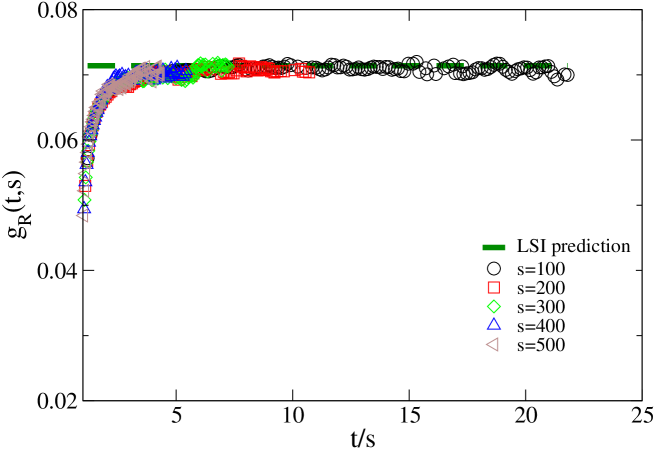
Figure 3: (Color on line) $g_{R}(t,s)$ defined in Eq.(37) with $\theta=0.38$ and $a=0.115$ in the the $d=2$ Ising model quenched to $T=T_{C}\simeq 2.26918J$. The broken line is the prediction of LSI.

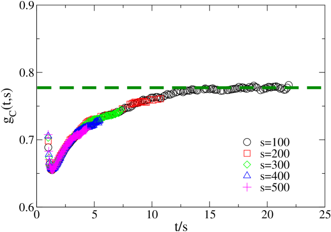
Figure 4: (Color on line) $g_{C}(t,s)$ defined in Eq.(38) with $\theta=0.38$ and $a=0.115$ in the the $d=2$ Ising model quenched to $T=T_{C}\simeq 2.26918J$. The broken line corresponds to the amplitude $A_{C}=0.78$.

We consider a square lattice with $N=1000^{2}$ Ising spins and we compute numerically the response and correlation functions in the quench to $T_{C}\simeq 2.26918J$, for five different values of $s=100,200,300,400,500$. In Fig.3 and Fig.4 we have plotted the quantities

$$g_{R}(t,s)=(t-s)^{a+1}(t/s)^{-\theta}R(t,s)$$ (37)

$$g_{C}(t,s)=(t-s)^{b}(t/s)^{1-\theta}C(t,s)$$ (38)

versus $t/s$, with $\theta=0.38$ and $a=b=0.115$ taken from ref. Pleimling . We find data collapse as expected from the RG results of Eqs. (2,13) which yield

$$g_{C}(t,s)=A_{C}f_{C}(t/s),\hskip 8.5359ptg_{R}(t,s)=A_{R}f_{R}(t/s).$$ (39)

Using, next, the asymptotic conditions $\lim_{x\to\infty}f_{R}(x)=\lim_{x\to\infty}f_{C}(x)=1$ we can extract the amplitudes $A_{C}=0.78\pm 0.02$ and $A_{R}=0.071\pm 0.002$. Lastly, from Fig.3 we can make a check on the LSI prediction (6) that $g_{R}(t,s)$ ought to be constant with $g_{R}(t,s)\equiv A_{R}$. Fig.3 shows that there is an evident deviation from LSI for $x<5$, while the LSI behavior holds for $x>5$.

IV.3 The limit fluctuation dissipation ratio $X_{\infty}$

We measure $X_{\infty}$ using Eq. (16) with values for $A_{C}$, $T_{C}A_{R}$ and $\theta$ estimated from the numerical data. In $d=4$, with $\theta=0$, $A_{C}=0.72\pm 0.02$ and $T_{C}A_{R}=0.35\pm 0.02$, we find $X_{\infty}=0.49\pm 0.03$ in agreement with the Gaussian result $X_{\infty}=1/2$. This supports the idea that not only $\theta$, but also $X_{\infty}$ is universal God ; Cala1 ; Cala1b .

In $d=2$, we find $A_{C}=0.78\pm 0.02$, $T_{C}A_{R}=0.161\pm 0.001$ and taking $\theta=0.38$ from Ref. Pleimling we obtain $X_{\infty}=0.33\pm 0.01$, in agreement with previous numerical results obtained with different methods Chat ; Sollich and with $X_{\infty}=0.30\pm 0.05$ from the two loop $\epsilon$ expansion Cala2 . For convenience, the numerical values of exponents, amplitude ratio and $X_{\infty}$ in the different processes have been collected in Table 1.

IV.4 $d=2$, $T<T_{C}$

In the quench to below $T_{C}$ the behavior of the data in the short time separation regime $t-s\ll s$ allows to discriminate between the additive and the multiplicative forms of $R(t,s)$. Expanding up to first order in $(t-s)/s$, in the former case from from Eqs. (4) and (5) one ontains

$$R(t,s)=R_{st}(t-s)+s^{-(1+a)}\left[h_{R}(1)+h^{\prime}_{R}(1)\left({t-s\over s}\right)\right]$$ (40)

while from the LSI form

$$R_{LSI}(t,s)=A_{R}(t-s)^{-(1+a)}x^{\theta}$$ (41)

one gets

$$R_{LSI}(t,s)=A_{R}(t-s)^{-(1+a)}\left[1+\theta\left({t-s\over s}\right)\right].$$ (42)

Therefore, as $t-s$ becomes small with finite $s$, from Eq. (40) there remains an $s$ dependence due to $s^{-(1+a)}h_{R}(1)$, while from Eq. (42) there is no residual $s$ dependence.

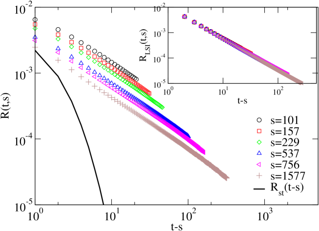
Figure 5: (Color on line) $R(t,s)$ in the quench of the Ising model to $T=1.5J$ below $T_{C}$. Inset: plot of $R_{LSI}(t,s)$ for the same values of $s$ and $t-s$. The continous line is the plot of $R_{st}(t-s)$.

In order to see which of the two behaviors is actually realized in the data, we have quenched a system of $1000^{2}$ Ising spins to the temperature $T=1.5J\simeq 0.69T_{C}$, taking the wide range of $s\in[101,1577]$ and focusing on the regime $t-s\leq s$. The numerical data are displayed in Fig.5. Furthermore, in the inset we have plotted Eq. (41) in the same range of $s$ and $t-s$, with $A_{R}=0.01$ obtained by imposing $R(s+1,s)=R_{LSI}(s+1,s)$ for $s=100$, $a=0.27$ extracted from the data for $R(t,s)$ (see below) and $\theta=\lambda/z-1-a$ with $\lambda/z=0.625$ LSI . The numerical data display an evident dependence on $s$ down to $t-s=1$, which is absent in those for $R_{LSI}(t,s)$ (note the same vertical scale). Therefore, the LSI form of $R(t,s)$ can be ruled out.

We have also extracted $R_{st}(t-s)$ from the data using the following protocol. We have let the system to evolve in contact with the thermal reservoir at the temperature $T=1.5J$ after preparing it in a completely ordered state, for instance all spins up. The equilibration time $t_{eq}$ for this process is finite and $R_{st}(t-s)$ is obtained by measuring the response function for $s>t_{eq}$. The data obtained in this way yield, as expected, an exponentially decaying contribution (continous line in Fig.5), which becomes very rapidly negligible with respect to the full $R(t,s)$. Therefore, in the observed range of $s$ and $t-s$, i) aging is well developed in the data and is due to the $R_{ag}(t,s)$ contribution in Eq. (4), while it is practically unobservable in the LSI and ii) the stationary contribution from the data decays exponentially, while in the LSI there is a power law decay.

Next, we have extracted $R_{ag}(t,s)$ via the subtraction $R_{ag}(t,s)=R(t,s)-R_{st}(t-s)$ and we have made the comparison with the fitting formula (25), which in the short time regime reads

$$R_{ag}(t,s)=A_{R}s^{-1/z}(t-s+t_{0})^{-1+1/z-a}\left[1+{\cal O}\left(\frac{t-s}{s}\right)\right].$$ (43)

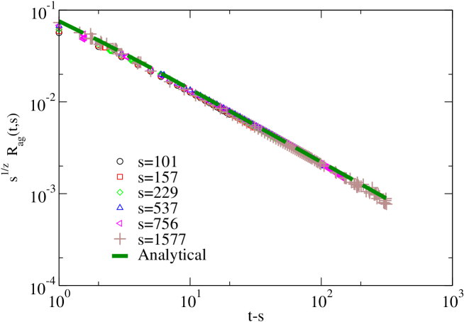
Figure 6: (Color on line) $s^{1/z}R_{ag}(t,s)$ with $z=0.47$ for the $d=2$ Ising model quenched to $T=1.5J$ below $T_{C}$. The broken line represents the power law behavior $(t-s+t_{0})^{-0.80}$ of $s^{1/z}R_{ag}(t,s)$ from Eq.(43).

and predicts TTI behavior if $s^{1/z}R_{ag}(t,s)$ is plotted against $t-s$. Indeed, this is observed in Fig.6, where we have used the exponent $1/z=0.47$ note obtained from the numerical data for the interface density $\rho_{I}(s)\sim s^{1/z}$. The curves for different values of $s$ collapse on a master curve which is very well fitted by the power law $(t-s+t_{0})^{-0.80}$ (broken line in Fig.6). The comparison with Eq. (43), then, gives the numerical value

$$a=0.27\pm 0.02$$ (44)

in agreement with previous results for this exponent noiachi ; noiRd2 . The tiny deviations from the fitting curve, observed in Fig.6 when $s$ is small and $t-s<2$, can be attributed to the absence of a sharp separation between bulk and interface fluctuations in this time regime. This implies that Eq. (4) is not exact for small $s$ and, therefore, that the aging contribution in the response function cannot be obtained simply by subtracting $R_{st}(t-s)$ from $R(t,s)$. However, this procedure becomes exact for larger values of $s$, as demonstrated by the fast convergence of the numerical data for $R_{ag}(t,s)$ towards the behavior of Eq. (43). Furthermore, as remarked above, the equilibrium response $R_{st}(t-s)$ is a very fast decreasing function of $t-s$ and, when $t-s>2$, the condition $R_{st}(t,s)\ll R(t,s)$ is fulfilled. Hence, even for small values of $s$, in the time region $t-s>2$, one has always $R(t,s)\simeq R_{ag}(t,s)$ and the numerical curves follow Eq. (43).

	$a$	$\theta$	$\frac{T_{C}A_{R}}{A_{C}}$	$X_{\infty}$
Gaussian model	(d-2)/2	0	1/2	1/2
Ising critical $d=4$	$1.01\pm 0.01$	$0.00\pm 0.02$	$0.49\pm 0.03$	$0.49\pm 0.03$
Ising critical $d=2$	0.115	0.38	$0.20\pm 0.01$	$0.33\pm 0.01$
Ising $T<T_{C}$ $d=2$	$0.27\pm 0.02$			0

Table 1: Exponents, amplitude ratio and $X_{\infty}$ for quenches to and to below $T_{C}$. The values of $a$ and $\theta$, in the $d=2$ critical quench of the Ising model, are taken from ref.Pleimling . For $X_{\infty}=0$ in the quench below $T_{C}$ see, for instance, ref.noiteff

.

V Conclusions

We have investigated the suggestion put forward in Ref. Cala1 ; Pleimling that LSI applies when Gaussian behavior holds, by looking at the scaling behavior of $R(t,s)$ in the kinetic Ising model with Glauber dynamics in two revealing test cases i) in the quench to $T_{C}$ with $d=4$, where deviations from Gaussian behavior are expected to disappear and ii) in the quench to $T_{C}$ and to below $T_{C}$ with $d=2$ where, conversely, corrections to Gaussian behavior are expected to become quite sizable. Unlike Pleimling and Gambassi, who work with an intermediate integrated response function, we have computed directly $R(t,s)$, in the sense specified in section III after Eq. (36), producing high precision data by means of the new numerical algorithm of ref. noialg . In the $d=4$ numerical simulation we have not found logarithmic corrections to the Gaussian behavior (see the insets of Fig.1 and Fig.2).

Our results do confirm the conjecture that a Gaussian approximation is inherent to LSI. In the case of the $d=4$ critical quench we find agreement between LSI, Gaussian behavior, and numerical data. Instead, in the case of the critical quench in $d=2$, deviations from LSI are observed, which go in the same direction as the field theoretical calculations and previous numerical results from the global integrated response functions. Similarly, important deviations from LSI behavior are found in the quench to below $T_{C}$. In the latter case the data i) are incompatible with the multiplicative form of $R(t,s)$ predicted by LSI and ii) do confirm the result $a=0.27\pm 0.02$ for the scaling exponent of $R_{ag}(t,s)$, first obtained from the measurements of $\chi(t,t_{w})$ noiachi . It ought to be mentioned that the behavior of $R_{ag}(t,s)$ in the quench to below $T_{C}$ of the $d=2$ Ising model has already been investigated numerically in great detail in ref. noiRd2 . In that paper we have produced evidence for the existence of a strong correction to scaling, next to the leading term behaving as in Eq. (5). In the present work there has been no need to worry about the correction to scaling, since we have focused on the time sector with $t-s<s$ and $s$ sufficiently large, where the correcting term is negligible noiRd2 .

Finally, it should also be mentioned that recently Henkel and collaborators LSI.1 ; LSI.2 have proposed a more general version of the LSI by replacing $F_{R}(x)$ in Eq. (1) with

$$F_{R}(x)=A_{R}\;(x-1)^{-(1+a^{\prime})}\;x^{\theta+a^{\prime}-a}$$ (45)

where $a^{\prime}$ is new exponent. The old LSI is contained in the new one as the particular case corresponding to $a^{\prime}=a$. Fitting the numerical data for the integrated response function in the critical quench of the $d=2$ Ising model LSI.2 , an improvement over the old LSI has been obtained with $a-a^{\prime}=0.187$. One of the problems with the new LSI, however, is that when $a\neq a^{\prime}$ the numerical improvement is obtained at the expense of destroying quasi stationarity in the short time regime, which is required by the separation of the time scales Cugliandolo . A detailed analysis of the new LSI is beyond the scope of the present work and is deferred to a future publication. Considerations similar to ours have been made by Hinrichsen Hinri in comparing numerical data with the predictions of LSI contact for the $1+1$-dimensional contact process.

Acknowledgments

This work has been partially supported by MURST through PRIN-2004.

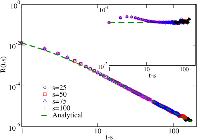
Figure 1: (Color on line) $R(t,s)$ in the $d=4$ Ising model quenched to $T=T_{C}\simeq 6.68J$. The broken line is the analytical solution of the Gaussian model (Eq.(22)) with $A_{R}=0.35/T_{C}$ and $t_{0}=0.1$.
Inset: plot of $(t-s+t_{0})^{2}R(t,s)$ showing the absence of corrections to Gaussian behavior. The broken line indicates the constant value.

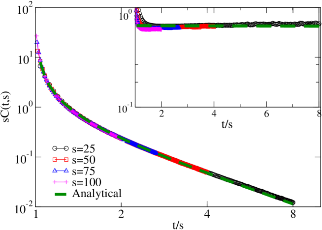
Figure 2: (Color on line) $C(t,s)$ in the $d=4$ Ising model quenched to $T=T_{C}\simeq 6.68J$. The broken line is the analytical solution of the Gaussian model (Eq.(21) with $A_{C}=0.72$ and $t_{0}=0.1$.
Inset: plot of $(x-1+t_{0}/s)(x+1+t_{0}/s)sC(t,s)$ showing the absence of corrections to Gaussian behavior. The broken line indicates the constant value.

References

- (1) For a review see J.P.Bouchaud, L.F. Cugliandolo, J. Kurchan and M. Mezard, in Spin Glasses and Random Fields edited by A.P. Young (World Scientific, Singapore,1997) A.Crisanti and F.Ritort, J.Phys.A: Math.Gen. 36, R181 (2003). L.F. Cugliandolo, in Slow Relaxation and Non Equilibrium Dynamics in Condensed Matter , J.-L. Barrat, J. Dalibard, J. Kurchan and M.V. Feigel’man (Eds.) Les Houches - Ecole d’Ete de Physique Theorique, Vol. 77/2004 Springer-Verlag. Also available as cond-mat/0210312.
- (2) L.F. Cugliandolo and J. Kurchan, Phys. Rev. Lett. 71, 173 (1993); J.Phys.A: Math.Gen. 27, 5749 (1994).
- (3) S.Franz, M.Mézard, G.Parisi and L.Peliti, Phys.Rev.Lett., 81, 1758 (1998); J.Stat.Phys. 97, 459 (1999).
- (4) H.K Janssen, B. Schaub and B. Schmittmann, Z. Phys. B Cond. Mat. 73 539 (1989).
- (5) P. Calabrese and A. Gambassi, Phys. Rev. E 65, 066120 (2002).
- (6) P. Calabrese and A. Gambassi, J. Phys. A 38, R133 (2005).
- (7) T. Ohta, D. Jasnow and K. Kawasaki, Phys.Rev.Lett., 49, 1225 (1982).
- (8) L.Berthier, J.L.Barrat and J.Kurchan, Eur.Phys.J.B 11, 635 (1999).
- (9) F. Corberi, E. Lippiello and M. Zannetti, Phys.Rev. E 63, 061506 (2001); Eur.Phys.J.B 24, 359 (2001).
- (10) G. Mazenko, Phys.Rev. E 69, 0116114 (2004).
- (11) E.Lippiello and M.Zannetti, Phys.Rev. E61, 3369 (2000).
- (12) C.Godrèche and J.M.Luck, J.Phys. A 33, 1151 (2000).
- (13) F. Corberi, E. Lippiello and M. Zannetti, Phys.Rev. E 65,046136 (2002);
- (14) M.Henkel, M.Pleimling, C.Godrèche and J.M.Luck, Phys.Rev.Lett. 87, 265701 (2001)
- (15) M.Henkel, Nucl.Phys. B 641, 405 (2002).
- (16) C.Godrèche and J.M.Luck, J.Phys. A 33, 9141 (2000)
- (17) F. Corberi, E.Lippiello and M. Zannetti, Phys.Rev.E 68, 046131 (2003).
- (18) P.Calabrese and A.Gambassi, Phys.Rev. E 67, 36111 (2002).
- (19) M. Pleimling and A.Gambassi, Phys.Rev. B 71, 180401 (2005).
- (20) C. Chatelain, J. Phys. A: Math.Gen., 36 10739 (2003).
- (21) F.Ricci-Tersenghi, Phys.Rev.E 68, 065104(R) (2003).
- (22) E. Lippiello, F. Corberi, and M. Zannetti, Phys.Rev.E 71, 036104 (2005).
- (23) K. Okano, L. Shülke, K. Yamagishi and B. Zheng,Nucl.Phys. B 485, 727 (1997); E. Arashiro and J.R. Drugowich de Felicio, Phys.Rev. E 67, 46123 (2002).
- (24) C. Chatelain, J. Stat. Mech. Theor. and Exp. P06006 (2004).
- (25) S.Abriet and D.Karevski, Eur.Phys.J.B 41, 79 (2004).
- (26) P.C. Hohenberg and B.I. Halperin, Rev.Mod.Phys 49,435 (1977).
- (27) L.F. Cugliandolo, J. Kurchan and G. Parisi J. Phys. I France 4, 1641 (1994).
- (28) F.Corberi, E.Lippiello and M.Zannetti, Phys.Rev.E 72, 056103 (2005).
- (29) F.Corberi, E.Lippiello and M.Zannetti, in preparation.
- (30) D.Stauffer and J.Adler, Int.J.Mod.Phys.C 8, 263 (1997).
- (31) P. Mayer, L. Berthier, J. P. Garrahan and P.Sollich, Phys.Rev.E 68, 016116 (2005).
- (32) To reach the asymptotic value requires very long simulations. For a value of similar to ours see, for instance, G.Manoj and P.Ray, Phys.Rev.E 62, 7755 (2000).
- (33) F.Corberi, E.Lippiello and M.Zannetti, J. Stat. Mech. Theor. and Exp. P12007 (2004).
- (34) M.Henkel, A.Picone and M.Pleimling, Europhys.Lett. 68, 191 (2004); M.Henkel and M.Pleimling, J.Phys.:Condens. Matter 17, S1899 (2005).
- (35) M.Henkel, T.Enss and M.Pleimling, cond-mat/0605211.
- (36) H.Hinrichsen, J.Stat.Mech. L06001 (2006).
- (37) T.Enss, M.Henkel, A.Picone and U.Schollwöck, J.Phys.A:Math.Gen. 37, 10479 (2004).