A Single Layer of Mn in a GaAs Quantum Well:
a Ferromagnet with Quantum Fluctuations

Abstract

Some of the highest transition temperatures achieved for Mn-doped GaAs have been in $\delta$-doped heterostructures with well-separated planes of Mn. But in the absence of magnetic anisotropy, the Mermin-Wagner theorem implies that a single plane of magnetic ions cannot be ferromagnetic. Using a Heisenberg model, we show that the same mechanism that produces magnetic frustration and suppresses the transition temperature in bulk Mn-doped GaAs, due to the difference between the light and heavy band masses, can stabilize ferromagnetic order for a single layer of Mn in a GaAs quantum well. This comes at the price of quantum fluctuations that suppress the ordered moment from that of a fully saturated ferromagnet. By comparing the predictions of Heisenberg and Kohn-Luttinger models, we conclude that the Heisenberg description of a Mn-doped GaAs quantum well breaks down when the Mn concentration becomes large, but works quite well in the weak-coupling limit of small Mn concentrations. This comparison allows us to estimate the size of the quantum fluctuations in the quantum well.

I Introduction

The discovery of dilute-magnetic semiconductors (DMS) with transition temperatures above 170 K Ohno96 ; Mun89 ; MacDon05 has renewed hopes for a revolution in semiconductor technologies based on electron spin Zutic04 . However, the difficulty in producing DMS materials with ferromagnetic transition temperatures above room temperature has stalled the development of practical spintronic devices. Some of the highest transition temperatures to date have been achieved in $\delta$-doped GaAs heterostructures,Naz05 where the Mn are confined to isolated planes. The Curie temperature of digital heterostructures does not seem to vanish as the distance between layers increases Kaw00 . Yet a single layer of magnetic ions with spin $S=5/2$ would not be expected to become ferromagnetic due to the Mermin-Wagner theorem, which states that gapless spin excitations destroy magnetic order at any nonzero temperature in two dimensions. The magnetic anisotropy due to strain is commonly invoked Lee00 ; Abol01 ; Liu03 ; Prio05 to explain the ferromagnetism of heterostructures. However, strain changes significantly as a function of film thickness and capping layers, and would be negligible for a single layer of Mn in a GaAs quantum well. The questions addressed in this paper are: can a single layer of Mn in a GaAs quantum well be ferromagnetic and what kind of ferromagnet is it?

To answer these questions, we employ two complementary approaches. First, we study the magnetic interactions between Mn moments embedded in a GaAs quantum well using a two-dimensional (2D) $S=5/2$ Heisenberg model, with exchange interactions taking the same form as in bulk Mn-doped GaAs.Zar02 Remarkably, the same anisotropic Heisenberg interactions that suppress the bulk transition temperature act to stabilize long-range magnetic order in 2D by producing a gap in the spin-wave (SW) spectrum. Second, we estimate the parameters of the Heisenberg model by constructing a Kohn-Luttinger (KL) model for a GaAs quantum well with an additional exchange interaction between the holes and the Mn spins, which are treated classically and confined to the central plane. Comparing the predictions of the Heisenberg and KL plus exchange (KLE) models, we conclude that the Heisenberg description of a Mn-doped quantum well works quite well for small Mn concentrations or in the weak-coupling limit, but breaks down when the Mn concentration becomes too large

This paper is organized into five sections. In Section II, we examine several anisotropic $S=5/2$ Heisenberg models that might describe a single layer of Mn in a GaAs quantum well. Section III develops a more precise electronic description of the quantum well based on the KLE model. In Section IV, the KLE model is used to estimate the parameters of an anisotropic Heisenberg model. A brief conclusion is provided in Section V.

II Heisenberg description of a Quantum Well

In bulk Mn-doped GaAs, the difference between the light ($m_{l}=0.07m$) and heavy ($m_{h}=0.5m$) band masses with ratio $r=m_{l}/m_{h}\approx 0.14$ produces an anisotropic interaction Zar02 between any two $S=5/2$ Mn ions. This anisotropy arises because the kinetic energy $K=\sum_{{\bf k},\alpha\beta}\epsilon({\bf k})_{\alpha\beta}c_{{\bf k},\alpha}^{\dagger}c_{{\bf k}\beta}$ is only diagonalized when the angular momentum ${\bf j}$ of the charge carriers is quantized along the momentum direction $\hat{\bf k}$. The heavy and light holes carry angular momentum ${\bf j}\cdot\hat{\bf k}=\pm 3/2$ and $\pm 1/2$, respectively. As shown by Zaránd and Jankó,Zar02 the interaction between Mn spins ${\bf S}_{i}$ and ${\bf S}_{j}$ (as in the inset to Fig. 1) can be written

$$H_{ij}=-J_{ij}^{(1)}{\bf S}_{i}\cdot{\bf S}_{j}+J_{ij}^{(2)}{\bf S}_{i}\cdot{\bf r}_{ij}\,{\bf S}_{j}\cdot{\bf r}_{ij}.$$ (1)

For $r=1$, $K$ is diagonal in any basis and $J_{ij}^{(2)}=0$. Since $J_{ij}^{(2)}>0$ for $r<1$, the Mn spins in GaAs prefer to align perpendicular to the vector ${\bf r}_{ij}=({\bf R}_{i}-{\bf R}_{j})/|{\bf R}_{i}-{\bf R}_{j}|$ connecting spins $i$ and $j$. For a tetrahedron of Mn spins, the interaction energy between every pair of spins cannot be simultaneously minimized and the system is magnetically frustrated. As shown both in the weak-coupling, RKKY limit Zar02 and more generally Ary05 ; Mor06 within dynamical mean-field theory, this anisotropic interaction suppresses the Curie temperature compared to a non-chiral system with $r=1$. Moreno et al. Mor06 found that the transition temperature may be lowered by about 50% for $r=0.14$ compared to $r=1$.

We construct a simple 2D Heisenberg model for a single layer of Mn-doped GaAs by including the effect of this anisotropy:

$$H^{ZJ}=\frac{1}{2}\sum_{i\neq j}H_{ij}-D\sum_{i}(S_{i}^{z})^{2}$$ (2)

where the sum is taken over a square lattice and $S=5/2$. We also include a single-ion anisotropy term $D$ that might be important in a quantum well due to elastic strain and spin-orbit coupling. When $J_{ij}^{(2)}>0$, the anisotropic interactions cause the Mn spins to point out of the plane, producing a gap $\Delta_{{\rm SW}}$ in the SW spectrum even when $D=0$. By breaking the rotational invariance of the spin, the anisotropic coupling would allow a single layer of Mn ions to order ferromagnetically even in the absence of single-ion anisotropy. As discussed further below, the single-ion anisotropy $D$ is also known Erick91 to produce a SW gap and to stabilize ferromagnetic long-range order in the 2D Heisenberg model.

Before proceeding to study $H^{\rm ZJ}$ using SW theory, we note that other types of Heisenberg models may also stabilize ferromagnetic order in 2D. For example, the Hamiltonian

$$H^{\prime}=-J\sum_{\langle i,j\rangle}\Bigl{\{}S_{i}^{x}S_{j}^{x}+S_{i}^{y}S_{j}^{y}+(1+\gamma)S_{i}^{z}S_{j}^{z}\Bigr{\}}$$ (3)

with an anisotropic coupling between neighboring spins was recently used Prio05 to model a plane of Mn spins in a GaAs host. When $\gamma\neq 0$, the rotational invariance of the spins is broken and 2D ferromagnetism is stabilized at finite temperatures. However, $H^{\prime}$ does not contain the same anisotropic interactions between Mn spins that are believed Zar02 to be present in the bulk system.

Due to the presence of the $J^{(2)}_{ij}$ terms in $H_{ij}$, $H^{\rm ZJ}$ does not commute with the total spin ${\bf S}_{{\rm tot}}=\sum_{i}{\bf S}_{i}$. Therefore, quantum fluctuations will suppress the magnetic moment of the ZJ model even at zero temperature. Such quantum fluctuations are typically found in antiferromagnets but are rather unusual in ferromagnets away from quantum critical points. Notice that the Hamiltonian $H^{\prime}$ constructed above does not have quantum fluctuations.

To gain a better idea of the size of the quantum fluctuations in the ZJ model, we specialize to the case where both $J^{(1)}_{ij}\equiv J_{1}$ and $J^{(2)}_{ij}\equiv J_{2}$ couple only neighboring spins on the square lattice. We then use SW theory to solve $H^{\rm ZJ}$, assuming that $S\gg 1$. At the mean-field ($1/S^{0}$) level, the ferromagnetic alignment of the spins along the $z$ axis is unstable to an A-type antiferromagnetic realignment of the spins in the $xy$ plane (with lines of spins alternating in orientation) when $J_{2}/J_{1}>2+D/J_{1}$. To order $1/S$, Eq. (1) may be written in terms of Holstein-Primakoff bosons:

$$H_{ij} \approx -J_{1}\Bigl{\{}{S^{2}-S(a_{i}^{\dagger}a_{i}+a_{j}^{\dagger}a_{j}-a_{i}^{\dagger}a_{j}-a_{j}^{\dagger}a_{i})}\Bigr{\}}$$ (4)

$$\pm \frac{J_{2}S}{2}(a_{i}\pm a_{i}^{\dagger})(a_{j}\pm a_{j}^{\dagger}),$$

where $\pm$ is $+$ for spin $i$ and $j$ separated by $\hat{x}$, and $-$ for spin $i$ and $j$ separated by $\hat{y}$. The second term in Eq. (2) will similarly contribute $2DS\sum_{i}a_{i}^{\dagger}a_{i}$. Since only the first terms in a $1/S$ expansion of the spin operators have been retained, the interactions between SW’s have been neglected. Because of the relatively large $S=5/2$ spin of the magnetic ions, however, the next order in the expansion ($1/S^{2}$) will be rather small for low temperatures, and we expect the linear approximation to recover all of the relevant quantum physics. Writing the Holstein-Primakoff bosons in a momentum representation, we get the useful form:

$$H^{\rm ZJ} = H_{0}+\sum_{{\bf k}}A_{{\bf k}}\left({a^{\dagger}_{{\bf k}}a_{{\bf k}}+a^{\dagger}_{-{\bf k}}a_{-{\bf k}}}\right)$$ (5)

$$+ \sum_{{\bf k}}B_{{\bf k}}\left({a^{\dagger}_{{\bf k}}a^{\dagger}_{-{\bf k}}+a_{{\bf k}}a_{-{\bf k}}}\right),$$

with coefficients given by

$$A_{{\bf k}} = 2J_{1}S\left[{1-\xi({\bf k})}\right]+J_{2}S\xi({\bf k})+DS$$

$$B_{{\bf k}} = J_{2}S\phi({\bf k})/2,$$ (6)

where $\xi({\bf k})=(\cos{k_{x}}+\cos{k_{y}})/2$ and $\phi({\bf k})=\cos{k_{x}}-\cos{k_{y}}$ (lattice constant set to unity). In this form, it is easy to see that the anisotropy $J_{2}$ destroys the ability of the Hamiltonian to commute with the total spin $S_{{\rm tot}}^{z}=\sum_{i}S^{z}_{i}=NS-\sum_{{\bf k}}a^{\dagger}_{{\bf k}}a_{{\bf k}}$, causing a quantum correction to the ground state magnetization.

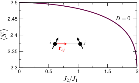
Figure 1: (color online) Quantum correction to the ground state magnetization per spin ($S=5/2$) in the limit $D=0$. The inset illustrates the direction of the interaction $J_{ij}^{(2)}$.

The SW Hamiltonian can be diagonalized in the usual way by transforming to Bogoliubov bosons $\alpha^{\dagger}_{\bf k}$ and $\alpha_{\bf k}$, which obey the canonical commutation relations. Forcing the resulting Hamiltonian to be diagonal in $\alpha^{\dagger}_{\bf k}\alpha_{\bf k}$, we obtain the SW energies $\omega_{\bf k}=2\sqrt{A^{2}_{\bf k}-B^{2}_{\bf k}}$ with the energy gap $\Delta_{{\rm SW}}=2(J_{2}+D)S$. The absence of terms linear in the boson operators and the positive definiteness of the SW frequencies for $-D<J_{2}<2J_{1}+D$ guarantee that the ferromagnetic state with all spins aligned along the $z$ axis is stable against non-collinear rearrangements of the spins Sch02 . The diagonalized SW Hamiltonian may be used to estimate the quantum-mechanical correction to the ground-state magnetization. Starting with the magnetization written as $\langle S_{i}^{z}\rangle=S-N^{-1}\sum_{{\bf k}}\langle{a^{\dagger}_{{\bf k}}a_{{\bf k}}}\rangle,$ we find upon transforming to Bogoliubov bosons,

$$\langle S_{i}^{z}\rangle=S-\frac{1}{N}\sum_{\bf k}\biggl{\{}{\frac{A_{\bf k}}{\omega_{\bf k}}-\frac{1}{2}+\frac{2A_{\bf k}}{\omega_{\bf k}}\langle\alpha^{\dagger}_{\bf k}\alpha_{\bf k}\rangle}\biggr{\}}.$$ (7)

Since $n_{\bf k}=\langle\alpha^{\dagger}_{\bf k}\alpha_{\bf k}\rangle=1/({\textrm{e}}^{\beta\omega_{\bf k}}-1),$ Eq. (7) can be used to calculate the quantum correction to the ground-state magnetization by simply setting $\langle\alpha^{\dagger}_{\bf k}\alpha_{\bf k}\rangle=0$ and evaluating the integrals over ${\bf k}$. The result is plotted versus $J_{2}/J_{1}$ for $D=0$ in Fig. 1.

Within linear SW theory, Eq. (7) also affords us the simplest estimate for the transition temperature $T_{\rm C}$ of the nearest-neighbor $H^{\rm ZJ}$ model. Clearly, the transition temperature calculated within this formalism neglects the large quantitative corrections due to SW interactions. But including such interactions to second-order in $1/S$ would require additional approximations to handle the terms quartic in $\alpha^{\dagger}_{\bf k}$ and $\alpha_{\bf k}$. Since the precise value of $T_{\rm C}$ does not play a role in the subsequent discussion, we are satisfied that the correct qualitative trends (i.e. the stabilization of $T_{\rm C}$ at a finite value) are reproduced by linear SW theory. Including now both terms of Eq. (7), we can write the $T$-dependent order parameter as

$$\langle S_{i}^{z}\rangle=S+\frac{1}{2}-\frac{1}{N}\sum_{\bf k}{\frac{A_{\bf k}}{\omega_{\bf k}}\coth\left({\frac{\beta\omega_{\bf k}}{2}}\right)}.$$ (8)

We obtain $T_{\rm C}$ from the crossing point $\langle S_{i}^{z}\rangle=0$ for a given set of parameters $J_{2}/J_{1}$ or $D/J_{1}$ finiteT . The result is illustrated in Fig. 2, where $T_{\rm C}$ is scaled by the Weiss mean-field (MF) result, $T_{\rm C}^{(MF)}=4J_{1}S(S+1)/3$.

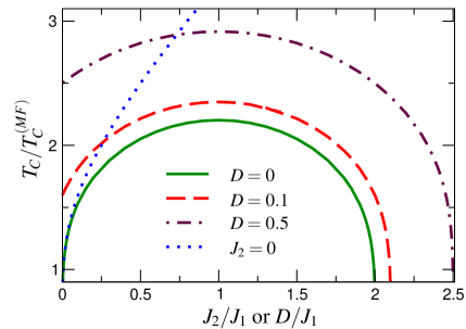
Figure 2: (color online) The transition temperature of the nearest-neighbor $H^{ZJ}$ model calculated in SW theory. For $D=0$, $T_{C}$ falls to zero at $J_{2}/J_{1}=0$ and 2 ; for $J_{2}=0$, $T_{C}=0$ for $D=0$ only. The SW value for $T_{\rm C}$ is normalized by the Weiss MF result.

Consider first the limiting case with $D=0$. Because the SW stiffness is assumed to be independent of temperature, the SW approach overestimates $T_{\rm C}$ for $J_{2}/J_{1}\approx 1$. Notice that $T_{\rm C}$ is symmetric on either side of $J_{2}/J_{1}=1$ and drops to zero when $J_{2}/J_{1}=0$ and 2. The limit $J_{2}/J_{1}\rightarrow 0$ can be analyzed by considering the behavior of the SW frequencies for small ${\bf k}$. Expanding $\omega_{\bf k}$ to second order in ${\bf k}$, we find that for small $J_{2}/J_{1}$, $T_{\rm C}\rightarrow 4\pi J_{1}S(S+1/2)/\ln(4\pi^{2}J_{1}/J_{2})$. This inverse logarithm is similar to the form discussed in Ref. [Erick91, ] for the $H^{\rm ZJ}$ model with $J_{2}=0$ and small single-ion anisotropy. In that case, $T_{\rm C}\rightarrow T_{3}/\ln(\pi^{2}J_{1}/D)$, where $T_{3}$ is the bulk transition temperature, approximately proportional to $J_{1}S(S+1)$.

We confirm this relationship by calculating $T_{C}$ in the $H^{\rm ZJ}$ model using the above SW theory, with $J_{2}=0$ and a nonzero $D$. As shown in Fig. 2, the results for $J_{2}=0$ or $D=0$ agree quite well as $D$ or $J_{2}\rightarrow 0$. For larger $J_{2}$ and $D$, the curves deviate significantly, with the $J_{2}=0$ curve growing linearly in the limit of large $D$. Quite generally, we find that as $\Delta_{{\rm SW}}\rightarrow 0$,

$$T_{\rm C}\rightarrow\frac{4\pi J_{1}S\left(S+1/2\right)}{\ln\left(8\pi^{2}J_{1}S/\Delta_{{\rm SW}}\right)}.$$ (9)

This general expression reduces to the correct limits when $J_{2}$ or $D=0$. We conclude that the behavior of $T_{\rm C}$ in the case of strong fluctuations is controlled by the isotropic exchange $J_{1}$ and the SW gap.

With a finite $D$, the $T_{\rm C}$ versus $J_{2}/J_{1}$ curve qualitatively resembles a scaled-up version of the $D=0$ curve in Fig. 2. In that case however, the asymptotic behavior at $J_{2}=0$ is removed ($T_{\rm C}$ becomes finite), the instability to in-plane ordering occurs at $J_{2}/J_{1}=2+D/J_{1}$ (as discussed above), and the maximum $T_{\rm C}$ increases. In our SW calculation, $T_{\rm C}$ vanishes at this instability due to the softening of the SW frequencies $\omega_{\bf k}$ with ${\bf k}=(\pi,0)$ and ${\bf k}=(0,\pi)$.

III The Kohn-Luttinger plus exchange model

To estimate the size of the quantum fluctuations in a Mn-doped GaAs quantum well, we model the quasi-2D hole gas as a thin quantum well of width $L$ accounting for the Coulomb confinement potential arising from the ionized dopants reboredo93 , central cell corrections, and any additional epitaxial confinement. We use a spherical approximation of the KL Hamiltonian Bald73 with four bands (${\bf j}\cdot\hat{\bf k}=\pm 3/2$ and $\pm 1/2$) to evaluate the energies $\epsilon({\bf k})_{\alpha\beta}$ for a GaAs quantum well with zero boundary conditions at $z=\pm L/2$. We express the Kohn-Luttinger Hamiltonian in a reduced basis form by the lowest-energy wavefunctions $\psi_{1}(z)=\sqrt{2/L}\cos(\pi z/L)$ and $\psi_{2}(z)=\sqrt{2/L}\sin(2\pi z/L)$ of the quantum well, with $\langle n|k_{z}^{2}|m\rangle=(n\pi/L)^{2}\delta_{nm}$. The Mn spins are now treated classically and the Mn impurities are distributed in the $z=0$ plane with concentration $c$. Since $\psi_{2}(0)=0$, the Mn spins only couple to the holes in the first wavefunction with projection $|\psi_{1}(0)|^{2}=2/L$. The exchange coupling of the Mn spins ${\bf S}_{i}=S{\bf m}_{i}$ with the holes is given by $V=-2J_{c}\sum_{i}{\bf m}_{i}\cdot{\bf j}_{i}$, where ${\bf j}_{i}=\sum_{\alpha\beta}c_{i,\alpha}^{\dagger}{\bf J}_{\alpha\beta}c_{i,\beta}/2$ are the hole spins and ${\bf J}_{\alpha\beta}$ are the Pauli spin-3/2 matrices. The states $\psi_{1}$ and $\psi_{2}$ are coupled by the off-diagonal terms in the KL Hamiltonian with matrix elements proportional to $\langle n|(k_{x}\pm ik_{y})k_{z}|m\rangle$, which vanishes for $n=m$ but is given by $-(8i/3L)(k_{x}\pm ik_{y})$ for $n=1$ and $m=2$.

For any coupling constant $J_{c}$ and orientation ${\bf m}=(\sin\theta,0,\cos\theta)$ of the Mn spins, the energy $E(J_{c},\theta)$ of the KLE model is obtained by first diagonalizing an $8\times 8$ matrix in $j=3/2$ and $n,m=1,2$ space:

$$H^{KLE}=\left(\begin{array}[]{cc}A_{1}&B^{\dagger}\\ B&A_{2}\end{array}\right).$$ (10)

The diagonal block elements can be written in terms of a generalized $4\times 4$ matrix,

$$A_{n}^{0}=\left(\begin{array}[]{cccc}\displaystyle\frac{k^{2}_{\perp}}{2m_{a}}+\left({\displaystyle\frac{n\pi}{L}}\right)^{2}\displaystyle\frac{1}{2m_{h}}+bQ_{\epsilon}&0&d(k_{x}-ik_{y})^{2}&0\\ 0&\displaystyle\frac{k^{2}_{\perp}}{2m_{b}}+\left({\displaystyle\frac{n\pi}{L}}\right)^{2}\displaystyle\frac{1}{2m_{l}}-bQ_{\epsilon}&0&d(k_{x}-ik_{y})^{2}\\ d(k_{x}+ik_{y})^{2}&0&\displaystyle\frac{k^{2}_{\perp}}{2m_{b}}+\left({\displaystyle\frac{n\pi}{L}}\right)^{2}\displaystyle\frac{1}{2m_{l}}-bQ_{\epsilon}&0\\ 0&d(k_{x}+ik_{y})^{2}&0&\displaystyle\frac{k^{2}_{\perp}}{2m_{a}}+\left({\displaystyle\frac{n\pi}{L}}\right)^{2}\displaystyle\frac{1}{2m_{h}}+bQ_{\epsilon}\end{array}\right),$$ (11)

so that $A_{1}=A_{1}^{0}-J_{c}{\bf m}\cdot{\bf J}$. We include the strain term $Q_{\epsilon}\equiv\epsilon_{zz}-(\epsilon_{xx}+\epsilon_{yy})/2$, which is multiplied by the deformation potential $b=-1.7$ eV for GaAs Dietl01 . The other block diagonal element is simply $A_{2}=A_{2}^{0}$, since the holes in $\psi_{2}(z)$ do not couple to the Mn spins at $z=0$. We have defined $d=\sqrt{3}(1/m_{h}-1/m_{l})/8$, ${\bf k}_{\perp}=(k_{x},k_{y})$, $m_{a}=4(3/m_{l}+1/m_{h})^{-1}$ and $m_{b}=4(1/m_{l}+3/m_{h})^{-1}$. The off-diagonal block elements coupling $\psi_{1}(z)$ and $\psi_{2}(z)$ are

$$B=\left(\begin{array}[]{cccc}0&{16id(k_{x}-ik_{y})}/{3L}&0&0\\ {16id(k_{x}+ik_{y})}/{3L}&0&0&0\\ 0&0&0&{-16id(k_{x}-ik_{y})}/{3L}\\ 0&0&{-16id(k_{x}+ik_{y})}/{3L}&0\end{array}\right),$$ (12)

which couples the $j_{z}=\pm 3/2$ and $\pm 1/2$ components.

An expression for $J_{c}$ can be derived by directly comparing the potential $V$ to the standard spin-hole interaction, e.g. Eq. (1) of Ref. [Dietl01, ]. We estimate

$$J_{c}\approx\displaystyle\frac{S(\beta N_{0})}{2j\Lambda}c,$$ (13)

where $S=5/2$, $j=3/2$, $\beta N_{0}\approx 1.2$ eV,Dietl01 , $\Lambda=L/a$ is the number of layers in the quantum well, and $a\approx 4$ $\overset{\circ}{\rm A}$ is the lattice constant of Ga in the $z=0$ plane. So we see that $J_{c}\approx 1\,c\,{\rm eV}/\Lambda$ is inversely proportional to the width of the quantum well. For $\Lambda=10$, $J_{c}\approx 100\,c$ meV.

The splitting between the light and heavy band masses at the $\Gamma$ point of $\psi_{n}(z)$ is given by

$$\Delta_{n}=\frac{1}{2}\left(\displaystyle\frac{n\pi}{\Lambda a}\right)^{2}\left({\frac{1}{m_{l}}-\frac{1}{m_{h}}}\right)-2bQ_{\epsilon}.$$ (14)

Since both contributions are positive for $Q_{\epsilon}<0$, the confinement of holes in the quantum well formally plays the same role as the compressive strain in a thin film.Saw04 For $\Lambda<20$ and typical strains less than 0.5%, the contribution to the band splitting from quantum confinement is much larger than the contribution from strain. In the limit $\Lambda\rightarrow 0$ of an infinitely narrow quantum well, the effects of strain can be neglected entirely. For a narrow quantum well with $\Lambda<20$, $\Delta_{n}\approx 29(n/\Lambda)^{2}$ eV and $J_{c}/\Delta_{1}\approx\Lambda c/29$. Hence, a narrow quantum well with a small Mn concentration is in the weak-coupling limit with $J_{c}\ll\Delta_{1}$. By contrast, GaAs films with $\Lambda$ larger than about 50 cannot be treated as quantum wells because too many wavefunctions $\psi_{n}(z)$ would be required. The dominant contribution to the band splitting in such films comes from strain Abol01 rather than the confinement of the holes.

After obtaining the eigenvalues of the $8\times 8$ matrix $H^{KLE}$, we evaluate the energy $E(J_{c},\theta)$ of a quantum well by integrating over ${\bf k}_{\perp}$. Since the hole filling $p$ in the region of perpendicular anisotropy is quite small, the holes only occupy a very small portion of the Brillouin zone centered around ${\bf k}_{\perp}=0$. This implies that each hole interacts with many different Mn moments, so that the precise geometry and location of the Mn impurities within the $z=0$ plane does not affect our results. Consequently, the results of the KLE model for the energy do not depend on whether the Mn ions are randomly distributed within the central plane. The small area in momentum space occupied by the holes also justifies our use of a spherical approximation Bald73 to the KL Hamiltonian.

Because each of the holes must interact with two Mn moments in order to mediate their effective interaction, the resulting quantum-well energy $E(J_{c},\theta)$ is an even function of $J_{c}$. Of course, magnetic properties like the Kondo effect do depend on the sign of the exchange coupling. But in the weak-coupling limit of small $J_{c}$, the Kondo temperature White07 will be extremely small and the Kondo effect shall be neglected in the subsequent discussion.

IV Estimation of the Heisenberg parameters

By comparing the predictions of the KLE and ZJ models, we now estimate the ZJ exchange interactions between the Mn moments in a GaAs quantum well. In general, obtaining the long-range interactions $J^{(1)}_{ij}$ and $J^{(2)}_{ij}$ that parameterize the ZJ Hamiltonian is not possible. However, we can estimate the ${\bf q}=0$ component of the isotropic exchange coupling, $J_{1}({\bf q}=0)=\sum_{j}J^{(1)}_{ij}$, by considering the change in energy of the quantum well when the exchange with the Mn spins (all aligned along the $z$ direction with angle $\theta=0$) is turned off. For $H^{\rm ZJ}$, this gives the energy to align all of the spins. So we find that

$$-\frac{1}{2}J_{1}({\bf q}=0)S^{2}-DS^{2}=\frac{1}{N}\Bigl{\{}E(J_{c},\theta=0)-E(J_{c}=0)\Bigr{\}}.$$ (15)

The ${\bf q}=0$ component of the anisotropic exchange coupling, $J_{2}({\bf q}=0)=\sum_{j}J^{(2)}_{ij}$, may be estimated by evaluating the change in energy when all of the Mn spins rigidly rotate away from the $z$ axis towards the $xy$ plane with angle $\theta$:

$$\frac{1}{4}J_{2}({\bf q}=0,\theta)S^{2}+DS^{2}=\frac{1}{N}\frac{E(J_{c},\theta)-E(J_{c},\theta=0)}{\sin^{2}\theta}.$$ (16)

Within the KLE model, the average exchange vanishes when the moments are randomly oriented (whether perpendicular or parallel to the plane) because holes with small momenta interact with many Mn moments. By contrast, the single-ion anisotropy energy $-D\sum_{i}(S_{i}^{z})^{2}$ is large when the moments are randomly oriented in the $z$ direction but vanishes when the moments are randomly oriented in the plane. Comparing the energies of these two random configurations, we conclude that the single-ion anisotropy $D$ corresponding to the KLE model must vanish. Because the right-hand side of Eq. (16) is independent of $\theta$ within the Hamiltonian Eq. (2), the proximity of $J_{2}({\bf q}=0,\theta\rightarrow 0)$ and $J_{2}({\bf q}=0,\pi/2)$ is a measure of how well the KLE model can be approximated by the Heisenberg model $H^{\rm ZJ}$.

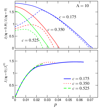
Figure 3: (color online) The top panel shows $J_{2}({\bf q}=0,\theta=0)/J_{1}({\bf q}=0)$ (dashed) and $J_{2}({\bf q}=0,\pi/2)/J_{1}({\bf q}=0)$ (solid) versus $p$ (holes per Mn) for three values of the Mn concentration $c$. In the bottom panel, $J_{1}({\bf q}=0)/J_{1}^{(0)}$ is plotted versus $p$ for the same concentrations.

Analytic results for the ${\bf q}=0$ exchange parameters can be obtained in the weak-coupling limit of small $J_{c}$ if only $\psi_{1}(z)$ is occupied by holes and the hole chemical potential $\mu\approx\pi pc/m_{a}a^{2}$ is also small compared to the band splitting $\Delta_{1}$. For $J_{c}\ll\mu\ll\Delta_{1}$, we find that $J_{1}({\bf q}=0)S^{2}=9\pi J_{c}^{2}/W\equiv J_{1}^{(0)}S^{2}$ and $J_{2}({\bf q}=0,\theta)=2J_{1}({\bf q}=0)$, where $W=\pi^{2}c/m_{a}a^{2}$ is the bandwidth and $m_{a}$ is the band mass in the $xy$ plane. Both $J_{1}({\bf q}=0)$ and $J_{2}({\bf q}=0,\theta)$ are independent of the hole filling due to the flatness of the 2D density-of-states Lee00 . Recall from our discussion above that the system with only nearest-neighbor interactions is unstable to an antiferromagnetic realignment of the spins in the $xy$ plane when $J_{2}/J_{1}>2$. So in the limit $J_{c}\ll\mu\ll\Delta_{1}$, a phase with aligned moments is unstable when the exchange interactions are short-ranged. Neglecting the effect of anisotropy, $J_{1}({\bf q}=0)$ may be used to estimate $T_{\rm C}$ from the MF solution of a spin $S$ Heisenberg model:

$$T_{\rm C}^{(MF)} = \frac{1}{3}J_{1}^{(0)}S(S+1)=\frac{1}{3\pi}(\beta N_{0})^{2}m_{a}a^{2}S(S+1)\frac{c}{\Lambda^{2}}$$ (17)

$$\approx 0.18\frac{c}{\Lambda^{2}}\,{\rm eV},$$ (18)

which agrees precisely with the MF result of Lee et al. Lee00 Hence, the transition temperature of a quantum well increases as it becomes narrower. A departure of the concentration $c(z)$ of the Mn profile from a delta function would increase the effective width of the confining potential, thereby lowering the transition temperature.

More generally, when both wavefunctions $\psi_{1}(z)$ and $\psi_{2}(z)$ are included, Eqs. (15) and (16) may be used to evaluate $J_{2}({\bf q}=0,\theta)/J_{1}({\bf q}=0)$ as a function of $p$. As illustrated in Fig. 3, $J_{2}({\bf q}=0,0)/J_{1}({\bf q}=0)$ initially increases with filling before decreasing and becoming negative above $p_{1}$ (indicating that the spins with $\theta=0$ are no longer locally stable). We find that $J_{1}({\bf q}=0)$ increases linearly for small $p$ and reaches a value of about 1.4 times $J_{1}^{(0)}$ at a filling $p\approx 0.025$, independent of $c$. The maximum in $J_{2}({\bf q}=0,0)/J_{1}({\bf q}=0)$ approaches 2 for small Mn concentrations $c$ and hole fillings $p$ approaching 0, which is just the limit $J_{c}\ll\mu\ll\Delta_{1}$ discussed above. By contrast, $J_{2}({\bf q}=0,\pi/2)/J_{1}({\bf q}=0)$ decreases with increasing $p$ and becomes negative when $p>p_{2}>p_{1}$. This implies that the moments are tilted away from the $z$ axis for $p>p_{1}$ and only fall into the $xy$ plane ($E(J_{c},\theta)$ has a minimum at $\theta=\pi/2$) above some higher filling $p_{3}>p_{2}$. Once the spins land on the $xy$ plane above $p_{3}$, the rotational invariance of the spins about the $z$ axis would destroy long-range magnetic order if not for crystal-field anisotropy within the plane Saw04 .

As remarked earlier, the Heisenberg description of a quantum well requires that $J_{2}({\bf q}=0,\theta)$ is independent of the angle $\theta$. Hence, Fig. 3 implies that for any nonzero Mn concentration, the ZJ model fails when the hole filling falls below a critical threshold. The ZJ model works best over the widest range of hole fillings for small Mn concentrations. For $c=0.175$, the ZJ model is appropriate for hole fillings in the range $0.025<p<0.07$. As $c$ increases, the Heisenberg description only works within a narrower range of hole fillings, and even there not as well. For Mn concentrations that are insufficiently small, the interactions between the Mn moments within the quantum well are too complex to be accounted for by the ZJ model, even when the exchange interactions are long-ranged.

Up to this point, we have not made any assumptions about the range of the interactions $J^{(1)}_{ij}$ and $J^{(2)}_{ij}$ in the ZJ model. When the Mn concentration is sufficiently low, we expect the nearest-neighbor interactions $J_{1}$ and $J_{2}$ to be the dominant ones and our results for $J_{1}({\bf q}=0)$ and $J_{2}({\bf q}=0,\theta)$ can be used to estimate the transition temperature of a quantum well. In Section II, we found that the transition temperature reaches a peak when $J_{2}=J_{1}$. So Fig. 3 suggests that the transition temperature of a quantum well will be highest for some hole filling slightly below $p_{1}$, when the moments still lie along the $z$ axis and $J_{1}({\bf q}=0)\approx J_{2}({\bf q}=0,\theta)$. For $c=0.175$, $T_{\rm C}$ will be go through a maximum when $p\approx 0.048$ holes per Mn.

V Conclusions

Our results imply that a single layer of Mn-doped GaAs (or a very thin film with $\delta$-doping) with perpendicular magnetic moments may achieve a transition temperature close to the MF result of Eq. (17). Figure 2 suggest that $T_{\rm C}$ will reach a maximum with increasing $p$ when $J_{2}({\bf q}=0,\theta)\approx J_{1}({\bf q}=0)$. At higher fillings, $T_{\rm C}$ is expected to decrease until the Mn moments fall into the $xy$ plane, whereupon crystal field anisotropy is required to stabilize long-range ferromagnetic order.

However, the description of a Mn-doped GaAs quantum well by a Heisenberg model, even one with long-range interactions, is restricted to small Mn concentrations and hole fillings that are above a threshold value. From Eq. (13), we see that this is just the weak-coupling limit $J_{c}\ll\Delta_{1}$ and $J_{c}\ll\mu$. As the Mn concentration increases, the Heisenberg description is valid over a narrower range of hole fillings and even within that range, is not as accurate. Recent work Fis06 on the double-exchange model also reached the conclusion that a mapping onto a Heisenberg model is only valid in the weak-coupling limit.

For small Mn concentrations, where the Heisenberg description works quite well, quantum fluctuations in the total spin may be at least partially responsible for the depression of the magnetic moment found in Mn-doped GaAs epilayers.Pot02 It is ironic that the same frustration mechanism that suppresses the Curie temperature and electronic polarization in bulk Mn-doped GaAs should permit ordering in a 2D quantum well. With these results, we are in a position to address our originally postulated questions: how can a single layer of Mn-doped GaAs be ferromagnetic, and what kind of ferromagnet is it? We conclude that a Mn-doped GaAs quantum well is ferromagnetic due to a SW gap produced by the difference between the light and heavy band masses, but quantum fluctuations suppress the $T=0$ moment of this ferromagnet from its fully saturated value.

It is a pleasure to acknowledge helpful conversations with Juana Moreno, Thomas Maier, and Adrian Del Maestro. This research was sponsored by the U.S. Department of Energy Division of Materials Science and Engineering under contract DE-AC05-00OR22725 with Oak Ridge National Laboratory, managed by UT-Battelle, LLC.

References

- (1) H. Ohno, A. Shen, F. Matsukura, A. Oiwa, A. Endo, S. Katsumoto and Y. Iye, Appl. Phys. Lett. 69, 363 (1996).
- (2) H. Munekata, H. Ohno, S. von Molnár, Armin Segmüller, L.L. Chang, and L. Esaki, Phys. Rev. Lett. 63, 1849 (1989).
- (3) For a recent review: A. H. MacDonald, P. Schiffer, and N. Samarth, Nature Materials 4, 195 (2005).
- (4) I. utić, J. Fabian, S. Das Sarma, Rev. Mod. Phys. 76, 323 (2004).
- (5) A.M. Nazmul, S. Sugahara, and M. Tanaka, Phys. Rev. B 67, 241308(R) (2003); A.M. Nazmul, T. Amemiya, Y. Shuto, S. Sugahara, and M. Tanaka, Phys. Rev. Lett. 95, 017201 (2005).
- (6) R.K. Kawakami, E. Johnston-Halperin, L.F. Chen, M. Hanson, N. Guébels, J.S. Speck, A.C. Gossard, and D.D. Awschalom, Appl. Phys. Lett. 77, 2379 (2000).
- (7) B. Lee, T. Jungwirth, and A.H. MacDonald, Phys. Rev. B 61, 15606 (2000).
- (8) M. Abolfath, T. Jungwirth, J. Brum, and A.H. MacDonald, Phys. Rev. B 63, 054418 (2001).
- (9) X. Liu, Y. Sasaki, and J.K. Furdyna, Phys. Rev. B 67, 205204 (2003).
- (10) D.J. Priour, Jr., E.H. Hwang, and S. Das Sarma, Phys. Rev. Lett. 95, 037201 (2005).
- (11) G. Zaránd and B. Jankó, Phys. Rev. Lett. 89, 047201 (2002); G.A. Fiete, G. Zaránd, B. Jankó, P. Redlínski, and C. Pascu Moca, Phys. Rev. B 71, 115202 (2005).
- (12) K. Aryanpour, J. Moreno, M. Jarrell, and R.S. Fishman, Phys. Rev. B 72, 045343 (2005).
- (13) J. Moreno, R.S. Fishman, and M. Jarrell, Phys. Rev. Lett 96, 237204 (2006).
- (14) J. Schliemann and A.H. MacDonald, Phys. Rev. Lett. 88 (2002).
- (15) R.P. Erickson and D.L. Mills, Phys. Rev. B 43, 11527 (1991).
- (16) P. Arovas and A. Auerbach, Phys. Rev. 38, 316 (1988); V. Yu. Irkhin, A. A. Katanin and M. I. Katsnelson, Phys. Lett. A, 157, 295 (1991).
- (17) F. A. Reboredo and C. R. Proetto, Phys. Rev. B 47, 004655 (1993).
- (18) A. Balderischi and N.O. Lipari, Phys. Rev. B 8, 2697 (1973).
- (19) T. Dietl, H. Ohno, and F. Matsukura, Phys. Rev. B 63, 195205 (2001).
- (20) M. Sawicki, F. Matsukura, A. Idziaszek, T. Dietl, G.M. Schott, C. Ruester, C. Gould, G. Karczewski, G. Schmidt, and L.W. Molenkamp, Phys. Rev. B 70, 245325 (2004); M. Sawicki, K.-Y. Wang, K.W. Edmonds, R.P. Campion, C.R. Staddon, N.R.S. Farley, C.T. Foxon, E. Papis, E. Kamińska, A. Piotrowska, T. Dietl, and B.L. Gallagher, Phys. Rev. B 71, 121302(R) (2005).
- (21) See, for example, R.M. White, Quantum Theory of Magnetism (Springer, New York, 2007), p. 129.
- (22) R.S. Fishman, F. Popescu, G. Alvarez, T. Maier, and J. Moreno, Phys. Rev. B 73, 140405(R) (2006).
- (23) S.J. Potashnik, K.C. Ku, R. Mahendiran, S.H. Chun, R.F. Wang, N. Samarth, and P. Schiffer, Phys. Rev. B 66, 012408 (2002).