Full counting statistics for the Kondo dot in the unitary limit

Abstract

We calculate the charge transfer probability distribution function $\chi(\lambda)$ for the Kondo dot in the strong coupling limit within the framework of the Nozières–Fermi–liquid theory of the Kondo effect. At zero temperature, the ratio of the moments $C_{n}$ of the charge distribution to the backscattering current $I_{{\rm bs}}$ follows a universal law $C_{n}/2I_{{\rm bs}}=(-1)^{n}(1+2^{n})/6$. The functional form of $\chi(\lambda)$ is consistent with tunnelling of electrons and, possibly, electron pairs. We then discuss the cross-over behaviour of $\chi(\lambda)$ from weak to strong Coulomb repulsion in the underlying Anderson impurity model and relate this to the existing results. Finally, we extend our analysis to the case of finite temperatures.

The importance of the noise spectra in charge transport has been recognised long ago Schottky . The higher moments of the charge distribution, however, are only just becoming accessible experimentally Reulet . The probability $P(Q)$ of charge $Q$ being transmitted through the system during the measuring time ${\cal T}$ and the respective moment generating function $\chi(\lambda)=\sum_{Q}e^{i\lambda Q}P(Q)$ have been established by Levitov and Lesovik Levitov for non-interacting electrons. The effects of electron–electron correlations on the counting statistics are currently a subject of intensive debate. In particular, a universal result that the linear response, zero–temperature statistics is binomial for any interacting system with one conducting channel has recently emerged Gogolin .

An important test system of such type is the so–called Kondo dot: a semiconductor quantum dot device in the Kondo regime. Extensive experimental Goldbaher-Gordon and theoretical Kaminski ; Pustilnik inquiries into conducting properties of these systems have recently taken place. In the last few weeks, two works appeared, Ref. Sela and Ref. Golub , where the zero–temperature shot noise is calculated for such devices in the strong–coupling limit.

In this Letter we widen the investigation and calculate the full charge distribution function (which encodes all the moments) in the strong–coupling Kondo regime. We also discuss the temperature corrections and make contact with the previous results for the Anderson impurity model Gogolin .

A good place to start is indeed the Hamiltonian for a single level quantum dot (which is a version of the Anderson impurity model)

$$H=H_{0}+H_{{\rm T}}+H_{{\rm C}}\;,$$ (1)

where

$$H_{0}=\sum\limits_{p,\sigma,\kappa}(\varepsilon_{p}-\mu_{\kappa})\psi^{\dagger}_{p,\sigma,\kappa}\psi^{\phantom{\dagger}}_{p,\sigma,\kappa}+\sum\limits_{\sigma}(\Delta_{0}+\sigma h)d^{\dagger}_{\sigma}d^{\phantom{\dagger}}_{\sigma}\;,$$ (2)

describes the conducting leads, $\psi^{\dagger}_{p,\sigma,\kappa}$ being the creation operator for the electron with momentum $p$, spin $\sigma=\uparrow,\downarrow$, in the lead $\kappa=R/L$, with dispersion relation $\varepsilon_{p}$ such that the Fermi level density of states $\nu=\sum_{p}\delta(\varepsilon_{p})$ is finite (we set $E_{F}=0$ and $e=\hbar=k_{B}=1$ throughout), and the fermionic level $d^{\dagger}_{\sigma}$ at the energy $\Delta_{0}$ in magnetic field $h$. The leads are DC biased $\mu_{L}=-\mu_{R}=V/2\geq 0$. Further,

$$H_{{\rm T}}=\sum\limits_{\sigma}\left(\gamma_{L}d^{\dagger}_{\sigma}\psi^{\phantom{\dagger}}_{\sigma,L}+\gamma_{R}\psi^{\dagger}_{\sigma,R}d^{\phantom{\dagger}}_{\sigma}+{{\rm H.c.}}\right)$$ (3)

represents the local electron tunnelling between the leads and the dot (with, in general, different amplitudes $\gamma_{L}$ and $\gamma_{R}$) while $H_{{\rm C}}=Un_{\uparrow}n_{\downarrow}$ with $n_{\sigma}=d^{\dagger}_{\sigma}d^{\phantom{\dagger}}_{\sigma}$, stands for the Coulomb repulsion $U$. In equilibrium, this probably is the best studied model in the condensed matter theory. In particular, in the Kondo regime ($\Delta_{0}<0$, $U$ positive and large), the Schrieffer–Wolf type transformation Schrieffer , tailored to the lead geometry Kaminski , can be applied to result into a Kondo type or s-d exchange model.

For the Kondo model in the strong–coupling limit, when the spin on the dot is absorbed into the Fermi sea forming a singlet, Nozières Nozieres devised a Landau–Fermi–liquid description based on a ‘molecular field’ expansion of the phase shift of the s–wave electrons:

$$\delta_{\sigma}(\varepsilon)=\delta_{0}+\alpha\varepsilon+\phi^{a}(n_{\sigma}-n_{\bar{\sigma}})\;,$$ (4)

where $\delta_{0}=\pi/2$, $\alpha$ and $\phi^{a}$ are phenomenological parameters corresponding to the residual potential scattering and the residual interactions, respectively. These processes are generated by polarising the Kondo singlet and so are of the order $\sim 1/T_{K}$, where $T_{K}$ is the Kondo temperature. The specific heat coefficient is proportional to $\alpha/(\pi\nu)$ while the magnetic susceptibility is proportional to the sum $\alpha/(\pi\nu)+2\phi^{a}/\pi$. Simple arguments were advanced in Ref. Nozieres to the effect that, because the Kondo singularity is tied up to the Fermi level, there exists a relation $\alpha=2\nu\phi^{a}$ between the two processes in Eq. (4). In particular, this explains why the Wilson ratio is equal to $2$. Clearly, it is not difficult to write down a second quantised Hamiltonian describing the processes in Eq. (4). Before doing so let us remark that it is well known that there is no critical $U$ in the Anderson model (1) and the Fermi liquid approach is actually valid for all $U$ (see Hewson for a review).

The strong–coupling Hamiltonian that describes the scattering and interaction processes encoded in Nozières Eq. (4) is of the form $H=H_{0}+H_{{\rm sc}}+H_{{\rm int}}$. The free Hamiltonian here is

$$H_{0}=\sum\limits_{p,\sigma}\varepsilon_{p}(c^{\dagger}_{p,\sigma}c^{\phantom{\dagger}}_{p,\sigma}+a^{\dagger}_{p,\sigma}a^{\phantom{\dagger}}_{p,\sigma})+VQ\;,$$ (5)

where $c^{\dagger}$ is the creation operator for the s–wave electrons, $a^{\dagger}$ is the creation operator of the p–wave electrons, included in order to account for the transport Pustilnik , and the operator

$$Q=\frac{1}{2}\sum\limits_{p,\sigma}(c^{\dagger}_{p,\sigma}a^{\phantom{\dagger}}_{p,\sigma}+a^{\dagger}_{p,\sigma}c^{\phantom{\dagger}}_{p,\sigma})\;$$

stands for the (minus) charge transferred across the junction. The scattering term is

$$H_{{\rm sc}}=\frac{\alpha}{2\pi\nu T_{K}}\sum\limits_{p,p^{\prime},\sigma}(\varepsilon_{p}+\varepsilon_{p^{\prime}})c^{\dagger}_{p,\sigma}c^{\phantom{\dagger}}_{p^{\prime},\sigma}\;,$$ (6)

while the interaction term reads

$$H_{{\rm int}}=\frac{\phi}{\pi\nu^{2}T_{K}}c^{\dagger}_{\uparrow}c^{\phantom{\dagger}}_{\uparrow}c^{\dagger}_{\downarrow}c^{\phantom{\dagger}}_{\downarrow}\;,$$ (7)

where $c^{\phantom{\dagger}}_{\sigma}=\sum_{p}c^{\phantom{\dagger}}_{p,\sigma}$ and we have changed to the dimensionless amplitudes $\alpha$ and $\phi$, so that in the actual Kondo model $\alpha=\phi=1$ (in the intermediate calculations it is convenient to treat $\alpha$ and $\phi$ as free parameters though). By the nature of the strong–coupling fixed point, the operators $\alpha$ and $\phi$ are irrelevant in the renormalisation group sense and therefore the perturbative expansion in $\alpha$ and $\phi$ is expected to converge.

The charge measuring field $\lambda(t)$ [$\lambda(t)=\lambda\theta(t)\theta({\cal T}-t)$ on the forward path and $\lambda(t)=-\lambda\theta(t)\theta({\cal T}-t)$ on the backward pass of the Keldysh contour $C$], couples, in the Lagrangian formulation, to the current Levitov2 via a term in the action $\int dt\lambda(t)\dot{Q}(t)=-\int dt\dot{\lambda}(t)Q(t)$, which can be gauged away by the canonical transformation

$$\begin{array}[]{llll}c\to c_{\lambda}&=&\cos(\lambda/4)c-i\sin(\lambda/4)a\;,\\ a\to a_{\lambda}&=&-i\sin(\lambda/4)c+\cos(\lambda/4)a\;.\end{array}$$ (8)

We therefore reach an important conclusion that the charge measuring field enters this problem as a rotation of the strong–coupling basis of the s– and the p–states. While $H_{0}$ is invariant under this substitution, it should be performed in both the scattering and the interaction Hamiltonians, $H_{{\rm sc}}[c]+H_{{\rm int}}[c]\to H_{\lambda}=H_{{\rm sc}}[c_{\lambda}]+H_{{\rm int}}[c_{\lambda}]$, when calculating the statistics. It is easily checked that at the first order in $\lambda$: $H_{\lambda}=H_{{\rm sc}}+H_{{\rm int}}+(\lambda/4)\hat{I}_{{\rm bs}}+O(\lambda^{2})$, where $\hat{I}_{{\rm bs}}$ is the backscattering current operator

$$\hat{I}_{{\rm bs}}= - i\frac{\alpha}{4\pi\nu T_{K}}\sum\limits_{p,p^{\prime},\sigma}(\varepsilon_{p}+\varepsilon_{p^{\prime}})(c^{\dagger}_{p,\sigma}a^{\phantom{\dagger}}_{p^{\prime},\sigma}-a^{\dagger}_{p,\sigma}c^{\phantom{\dagger}}_{p^{\prime},\sigma})$$ (9)

$$- i\frac{\phi}{2\pi\nu^{2}T_{K}}\sum\limits_{\sigma}(c^{\dagger}_{\sigma}a^{\phantom{\dagger}}_{\sigma}-a^{\dagger}_{\sigma}c^{\phantom{\dagger}}_{\sigma})c^{\dagger}_{\bar{\sigma}}c^{\phantom{\dagger}}_{\bar{\sigma}}\;,$$

alternatively available from the commutator $\hat{I}_{{\rm bs}}=-\dot{Q}=i[Q,H]$.

The charge probability distribution function is therefore defined by

$$\chi(\lambda)=e^{iN\lambda}\left\langle T_{C}\exp\left[-i\int_{C}H_{\lambda}(t)dt\right]\right\rangle\;,$$ (10)

where $T_{C}$ is the time ordering operator on the Keldysh contour, and $N=(V{\cal T})/\pi=(2e^{2}/h)V{\cal T}$. Applying the standard linked cluster expansion (still valid on the Keldysh contour, of course)AGD , we see that the leading correction to the distribution function is given by a connected average

$$\ln\chi(\lambda)=iN\lambda-\frac{1}{2}\int_{C}dt_{1}dt_{2}\langle T_{C}\{H_{\lambda}(t_{1})H_{\lambda}(t_{2})\}\rangle_{{\rm c}}+...$$ (11)

The neglected terms $\alpha^{4}$, $\alpha^{2}\phi^{2}$, $\phi^{4}$, etc., are of the higher order in voltage (temperature) than the main correction because of the irrelevant nature of the perturbation. In order to make progress with Eq. (11), one only needs the Green’s function of the $\lambda$–rotated $c$–operator, which is easily seen to be the following matrix in Keldysh space

$$\hat{g}_{\lambda}(p,\omega)=i\pi\delta(\varepsilon_{p}-\omega)\left\{\right.[f(\omega-V/2)+f(\omega-V/2)-1]\hat{\tau}_{0}+[e^{-i\lambda/2}f(\omega-V/2)+e^{i\lambda/2}f(\omega+V/2)]\hat{\tau}_{+}$$ (12)

$$-[(1-f(\omega-V/2))e^{i\lambda/2}+(1-f(\omega+V/2))e^{-i\lambda/2}]\hat{\tau}_{-}\left.\right\}\;,$$

where $\hat{\tau}_{i}$ is the standard choice of Pauli matrices and $f(\omega)$ is the Fermi distribution function. We did not write the principal part which does not contribute to local quantities in the flat band model Lifshits .

The correction to the distribution function which is due to the scattering term (6) is shown in Fig. 1(a). The corresponding analytic expression is (a factor of 2 comes from summing over the spin index)

$$\delta_{\alpha}\ln\chi(\lambda) = -\frac{\alpha^{2}}{4\pi^{2}\nu^{2}T_{K}^{2}}\sum\limits_{p_{1},p_{2}}(\varepsilon_{p_{1}}+\varepsilon_{p_{2}})^{2}\int_{C}dt_{1}dt_{2}g_{p_{2}}(t_{2},t_{1})g_{p_{1}}(t_{1},t_{2})$$ (13)

$$= \frac{\alpha^{2}{\cal T}}{\pi T_{K}^{2}}\int d\omega\omega^{2}[(e^{-i\lambda}-1)n_{L}(1-n_{R})+(e^{i\lambda}-1)n_{R}(1-n_{L})]\;,$$

which, at zero temperature, contributes to Eq. (11) a term

$$\delta_{\alpha}\ln\chi(\lambda)=\frac{\alpha^{2}V^{3}{\cal T}}{12\pi T_{K}^{2}}(e^{-i\lambda}-1)\;.$$ (14)

Regarding the correction to the charge distribution coming from the interaction term (7), any diagrams with a single insertion of the Green’s function vanish (therefore there is also no $\alpha\phi$ cross term) and the only remaining connected graph is shown in Fig. 1(b). This is best calculated in real time. At zero temperature we have (no summation over the spin index):

$$\delta_{\phi}\ln\chi(\lambda)=-\frac{\phi^{2}}{2\pi^{2}\nu^{4}T_{K}^{2}}\int_{C}dt_{1}dt_{2}g(t_{1},t_{2})^{2}g(t_{2},t_{1})^{2}$$

$$= ~{}\frac{\phi^{2}}{\pi^{2}T_{K}^{2}}\int\limits_{-\infty}^{\infty}dt\frac{\cos^{4}[\lambda/2+(Vt)/2)]}{(t+i\alpha)^{4}}$$

$$= ~{}\frac{\phi^{2}V^{3}{\cal T}}{12\pi T_{K}^{2}}(e^{-i\lambda}-1)+\frac{\phi^{2}V^{3}{\cal T}}{6\pi T_{K}^{2}}(e^{-2i\lambda}-1)\;.$$

Combining the results we find that the zero–temperature charge distribution function is of the form:

$$\ln\chi(\lambda) = iN\lambda+\frac{V^{3}{\cal T}}{12\pi T_{K}^{2}}\left[(\alpha^{2}+\phi^{2})(e^{-i\lambda}-1)\right.$$ (16)

$$+ \left.2\phi^{2}(e^{-2i\lambda}-1)\right]+O(V^{5})\;.$$

In particular, the results of Golub for the average backscattering current and noise power are correctly reproduced (there the notation is $a=\alpha/(2\pi),b=\phi/\pi$). Therefore the Fano factor is equal to

$$\frac{C_{2}}{2I_{{\rm bs}}}=\frac{\alpha^{2}+9\phi^{2}}{2(\alpha^{2}+5\phi^{2})}\;,$$ (17)

which is $1/2$ for non-interacting electrons ($\phi=0$) and $5/6$ at the Kondo fixed point ($\alpha=\phi$).

But we now know much more – all the moments can be computed from Eq. (16) via $C_{n}=(-i)^{n}(d^{n}/d\lambda^{n})\ln\chi(\lambda)|_{\lambda=0}$, leading to

$$\frac{C_{n}}{2I_{{\rm bs}}}=(-1)^{n}\frac{\alpha^{2}+(1+2^{n+1})\phi^{2}}{2(\alpha^{2}+5\phi^{2})}\;,$$ (18)

$n=2,3,...$. Hence at $\alpha=\phi=1$ we have a hierarchy of universal (Fano factor inspired) ratios $C_{n}/2I_{{\rm bs}}=(-1)^{n}(1+2^{n})/6$.

In some systems, like in the case of the fractional quantum Hall effect, there are physical grounds on which to expect fractional charge quasiparticles to appear in transport depicciotto . In the present problem, which after all answers the Fermi liquid description, there are no such circumstances. In fact, the functional form of the distribution function allows a very simple interpretation. The term proportional to $V^{3}(\alpha^{2}+\phi^{2})(e^{-i\lambda}-1)$ must be interpreted as tunnelling of conventional electrons with charge $e$ (this is indeed obvious from the fact that at $\phi=0$ there is no interaction and the problem is trivial). It is tempting to interpret the term proportional to $V^{3}\phi^{2}(e^{-2i\lambda}-1)$, which appears as a result of electron correlations, as a coherent tunnelling of electron pairs with charge $2e$. [Certain caution is required here, as one can show that, at higher orders, a term of the form $V^{5}\alpha^{4}(e^{-2i\lambda}-1)$ exists, which is an artefact of the expansion around the perfect transmission.]

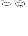
Figure 1: Schematic representation of the scattering (a), and interaction contributions (b).

Let us now return to the original model Eq. (1). There is an extensive vintage literature on the Fermi liquid properties of the equilibrium Anderson model Yamada1 . The perturbative expansion in the Coulomb repulsion $U$ can often be re-summed to all orders, using Ward identities and similar techniques, so that the observable quantities (specific heat, conductance, magnetisation) are expressed in terms of the even at odd susceptibilities $\chi_{e}$ and $\chi_{o}$ (correlations of $n_{\uparrow}$ with $n_{\uparrow}$ and $n_{\downarrow}$, respectively). These are universal functions of $U$ and are known exactly from the Bethe ansatz OK ; TW . Specifically, in the weak coupling $\chi_{{\rm e}}=1+(3-\pi^{2}/4)U^{2}/(\pi^{2}\Gamma^{2})+...$ and $\chi_{{\rm o}}=-U/(\pi\Gamma)$, where $\Gamma=2(\pi\nu\gamma)^{2}$ (we assume, for simplicity, a symmetric junction, $\gamma_{L}=\gamma_{R}=\gamma$ and particle–hole symmetry $\Delta_{0}=-U$). On the other hand, in the strong coupling we have: $\chi_{e}=(\Gamma\alpha)/(\pi T_{K})$ and $\chi_{o}=(\Gamma\phi)/(\pi T_{K})$, as here $\alpha=\phi=1$ and $T_{K}$ is the Kondo temperature up to a prefactor TW ; OK ; Hewson . The programme of extending a Fermi liquid approach to non-equilibrium properties of the Anderson model has not been comprehensively carried out yet.

There is a Fermi-liquid proof, due to Oguri Oguri , that the leading non-equilibrium correction to the zero–temperature current is of the form

$$I_{{\rm bs}}=\frac{V^{3}}{12\pi^{2}\Gamma^{2}}(\chi_{e}^{2}+5\chi_{o}^{2})\;,$$ (19)

which is valid for all $U$ and interpolates between the weak–coupling and the strong–coupling regimes of the Anderson model. We see that the above result for $I_{{\rm bs}}$ is simply the strong–coupling limit of Oguri’s formula.

As to the noise and higher moments no analogous Fermi–liquid results exist, to the best of our knowledge. However, in our recent paper Gogolin , we did put forward the formula for the charge distribution function:

$$\ln\chi(\lambda) = N\left\{i\lambda+\frac{V^{2}}{3\Gamma^{2}}\left[\frac{\chi_{e}^{2}+\chi_{o}^{2}}{4}(e^{-i\lambda}-1)\right.\right.$$

$$+ \left.\left.\frac{\chi_{o}}{2}(e^{-2i\lambda}-1)\right]\right\}\;,$$

which was a guess based on the properties of the perturbative expansion in $U$. In Gogolin we have shown that Eq. (Full counting statistics for the Kondo dot in the unitary limit) is correct at the order $U^{2}$ [it is also consistent with Eq. (19) for all $U$]. The calculations in this Letter prove that Eq. (Full counting statistics for the Kondo dot in the unitary limit) is also correct in the strong–coupling limit.

Before we close, we wish to discuss the effects a finite temperature $T$. The energy integral in Eq.(13) is elementary. The time integration in Eq. (Full counting statistics for the Kondo dot in the unitary limit) can also be done with standard methods (the real time Green’s function at $T>0$ is related to that at $T=0$ by a well known conformal mapping $1/t\to\pi T/\sinh(\pi Tt)$, see book ). The result for the generating function is:

$$\ln\chi(\lambda) = iN\lambda+\frac{V{\cal T}}{24\pi T_{K}^{2}}\left\{\frac{\alpha^{2}+\phi^{2}}{\sinh(V/2T)}[V^{2}+4(\pi T)^{2}][e^{V/2T}(e^{-i\lambda}-1)+e^{-V/2T}(e^{i\lambda}-1)]\right.$$ (21)

$$+ \left.\frac{2\phi^{2}}{\sinh(V/T)}[V^{2}+(\pi T)^{2}][e^{V/T}(e^{-2i\lambda}-1)+e^{-V/T}(e^{-2i\lambda}-1)]\right\}\;.$$

Using this formula we recover the finite-$T$ version of Eq. (19), see Oguri . The higher moments generated from Eq. (21), starting with $n=2$, are all new results (to our knowledge). The most important of these is the expression for the noise, which we here report:

$$C_{2}=\frac{V}{\pi T_{K}^{2}}\left\{\coth\left(\frac{V}{2T}\right)\left[\frac{\alpha^{2}+\phi^{2}}{12}V^{2}+\frac{\alpha^{2}+\phi^{2}}{3}\right.(\pi T)^{2}\right]+\left.\coth\left(\frac{V}{T}\right)\frac{2\phi^{2}}{3}\left[V^{2}+(\pi T)^{2}\right]\right\}\;.$$ (22)

To summarise, we have calculated the full counting statistics near the unitary strong–coupling limit of the Kondo dot. We wish to stress that Eq. (Full counting statistics for the Kondo dot in the unitary limit), even though correct for all the moments in both weak–coupling and strong–coupling limits, has not been formally proven yet. The theoretical challenge is to develop Fermi liquid theory for the counting statistics.

The authors participate in the European network DIENOW. AK is Feodor Lynen Fellow of the Alexander von Humboldt foundation.

References

- (1) W. Shottky, Ann. Phys. (Leipzig) 57, 541 (1918).
- (2) B. Reulet, J. Senzier, and D. E. Prober, Phys. Rev. Lett. 91, 136802 (2003). Y. Bomze, G. Gershon, D. Shovkun, L. S. Levitov, and M. Reznikov, Phys. Rev. Lett. 95 176601 (2005).
- (3) L. S. Levitov and G. B. Lesovik, JEPT Lett. 58, 230 (1993).
- (4) A. O. Gogolin and A. Komnik, Phys. Rev. B, in press, cond-mat/0512174. See this paper for further references on interaction effects.
- (5) D. Goldbacher-Gordon, H. Shtrikman, D. Mahalu, D. Abush-Magder, U. Meirav, and M. A. Kastner, Nature 391, 156 (1998). S. M. Cronenwett, T. H. Oosterkamp, and L. P. Kouwenhoven, Science 281, 540 (1998).
- (6) A. Kaminski, Yu. V. Nazarov, and L. I. Glazman, Phys. Rev. B 62, 8154 (2000).
- (7) M. Pustilnik and L. I. Glazman, cond-mat/0501007.
- (8) E. Sela, Y. Oreg, F. von Oppen, and J. Koch, cond-mat/0603442.
- (9) A. Golub, cond-mat/0603549.
- (10) J. R. Schrieffer and P. A. Wolf, Phys. Rev. 149, 491 (1966).
- (11) P. Nozières, J. of Low Temp. Phys., 17, 31 (1974).
- (12) A. C. Hewson, The Kondo Problem to Heavy Fermions (Cambridge University Press, 1993).
- (13) L. S. Levitov and M. Reznikov, Phys. Rev. B 70, 115305 (2004).
- (14) A. A. Abrikosov, L. P. Gor’kov, and I. E. Dzyaloshinskii, Methods of Quantum Field Theory in Statistical Physics (Prentice-Hall, Englewood, 1963).
- (15) E. M. Lifshits and L. P. Pitaevskii, Physical Kinetics (Pergamon Press, Oxford, 1981).
- (16) R. de Picciotto, M. Reznikov, M. Heiblum, V. Umansky, G. Bunin, and D. Mahalu, Nature (London) 389, 162 (1997). L. Saminadayar, D. C. Glattli, Y. Jin, and B. Etienne, Phys. Rev. Lett. 79, 2526 (1997).
- (17) K. Yamada, Prog. Theor. Phys. 53, 970 (1975); ibid 54, 316 (1975). K. Yosida and K. Yamada, Prog. Theor. Phys. 53, 1286 (1975).
- (18) N. Kawakami and A. Okiji, J. Phys. Soc. Jap. 51, 1145 (1982). A. Okiji and N. Kawakami, Solid State Comm. 43, 365 (1982).
- (19) P. B. Wiegmann and A. M. Tsvelick, J. Phys. C: Solid State Phys. 16, 2281 (1983). A. M. Tsvelick and P. B. Wiegmann, Phys. Lett. 89A, 368 (1982).
- (20) A. Oguri, Phys. Rev. B 64, 153305 (2001).
- (21) A. O. Gogolin, A. A. Nersesyan, and A. M. Tsvelik, Bosonization and Strongly Correlated Systems (Cambridge University Press, 1998).