Theoretical Analysis of the “Double-q” Magnetic Structure of CeAl₂

Abstract

A model involving competing short-range isotropic Heisenberg interactions is developed to explain the “double-q” magnetic structure of CeAl₂. For suitably chosen interactions terms in the Landau expansion quadratic in the order parameters explain the condensation of incommensurate order at wavevectors in the star of $(1/2-\delta,1/2+\delta,1/2)(2\pi/a)$, where $a$ is the cubic lattice constant. We show that the fourth order terms in the Landau expansion lead to the formation of the so-called “double-q” magnetic structure in which long-range order develops simultaneously at two symmetry-related wavevectors, in striking agreement with the magnetic structure determinations. Based on the value of the ordering temperature and of the Curie-Weiss $\Theta$ of the susceptibility, we estimate that the nearest neighbor interaction, $K_{0}$, is ferromagnetic with $K_{0}/k=-11\pm 1$K and the next-nearest neighbor interaction $J$ is antiferromagnetic with $J/k=6\pm 2$K. We also briefly comment on the analogous phenomena seen in the similar system, TmS.

I INTRODUCTION

CeAl₂ (CEAL) is a metallic system whose magnetic structure has been the object of some controversy for several years.CEAL1 ; CEAL2 ; CEAL3 ; CEAL4 ; CEAL5 ; CEAL6 Initial studiesCEAL1 ; CEAL2 indicated the existence of incommensurate long-range magnetic order on the Ce ions with a single wavevector in the star of ${\bf q}$, where

$${\bf q} = (2\pi/a)(1/2-\delta,1/2+\delta,1/2)\equiv(2\pi/a)\hat{\bf q}\ ,$$ (1)

with $\delta=0.11.$CEAL1 ; CEAL2 LaterCEAL3 it was proposed that this structure involved the simultaneous condensation of three wavevectors in the star of ${\bf q}$, but this suggestion of a “triple q” structure was refuted in Ref. CEAL4, . More recent workCEAL5 ; CEAL6 showed that the structure was in fact a “double q” one in which exactly two wavevectors in the star of ${\bf q}$ were simultaneously condensed. In addition, continued interest in CEAL is due to its Kondo-like behavior. Initial indications of this came from the observation of a minimum in the resistivity at about 15K, which was attributed to spin compensation.RES0 A single impurity model, with a Ce³⁺ ion in a cubic crystal field interacting with the conduction band, was able to account for most of the electrical properties.RES2 Moreover, when, in neutron experiments, no third order magnetic satellite appeared at low temperature, the Kondo effect was invoked to explain why the moment of a Kramers ion did not saturate in the zero-temperature limit.CEAL2 This objection is partially removed by the double-q structure.CEAL6 Moreover, an analysisOHKAWA of multi-q states claims that the double-q structure can not be explained if CEAL is regarded as an itinerant-electron magnet.

In this paper we proceed under the assumption that although Kondo effects may be present due to the coupling of the Ce 4f electron to the conduction band, the magnetic structure can be understood in terms of interaction between localized moments on the Ce ions. Since the lattice structure is fcc, it is apparent that antiferromagnetic interactions between shells of near neighbors could compete and might then explain the incommensurability. However, no concrete calculations of this type have yet appeared. It is also interesting that this system does not follow the simplest scenario for incommensurate magnets,Nagamiya namely, as the temperature is lowered, a phase transition occurs in which a modulated phase appears with spins confined to an easy axis, and then, at a lower temperature a second phase transition occurs in which transverse order develops, so as to partially satisfy the fixed length spin constraint expected to progressively dominate as the temperature is lowered. Instead, in CEAL, there is no second phase transition, and in the ordered phase one has the simultaneous condensation of long-range order at two symmetry-related wavevectors.CEAL5 ; CEAL6 There are two aspects of this behavior that have not yet been explained. 1) The incommensurate wavevector lies close to, but not exactly along the high symmetry $(1,1,1)$ direction and 2) although so-called “triple-q” systems are well known,3qa ; 3qb ; 3qc ; 3qd ; 3qe in which the incommensurate ordered state consists of the simultaneous superposition of three wavevectors, it is unusual, in a cubic system, to have a “double-q” statedq1 ; dq2 consisting of the simultaneous superposition of exactly two wavevectors.

The aim of this paper is to develop a model which can explain the above two puzzling features. We first address the determination of the incommensurate wavevector. Some time ago, Yamamoto and NagamiyaYN (YN) studied the ground state of a simple fcc antiferromagnet with isotropic nearest-neighbor (nn) and next-nearest neighbor (nnn) Heisenberg interactions and found a rich phase diagram in terms of these interactions whose coupling constants we will denote here as $J$ and $M$, respectively. We perform an equivalent calculation for a related model appropriate to CEAL based on an analysis of the terms in the Landau expansion of the free energy in the paramagnetic phase. By studying the instability of this quadratic form which occurs as the temperature is lowered, one can predict the magnetic structure of the ordered phase. In particular, one can thereby determine the wavevector at which this instability first occurs. This phenomenon is referred to as “wavevector selection.” As Nagamiya’s reviewNagamiya indicates, correct wavevector selection in CEAL must require a model which involves competition between nn and further neighbor interactions. For the fcc structure of CEAL the most convenient model which almost explains wavevector selection involves nn, nnn, and fourth-neighbor interactions. Based on our insight developed from this model, we suggest the how more general interactions can completely explain wavevector selection. Although we invoke more distant than nn interactions, the magnitudes of the further neighbor couplings needed to explain the nonsymmetric wavevector of CEAL decrease with increasing separation and are reasonable, especially in view of the possibility of Ruderman-Kittel-Kasuya-Yosida (RKKY)RK interactions in this metallic system. Because our main interest lies in explaining wavevector selection, we have completely ignored anisotropy, whose major effect is to break rotational invariance and select spin orientations. Coincidentally we note several regions in parameter space for these models in which one has a multiphase point (at which wavevector selection is incomplete). This phenomenon is perhaps most celebrated in the KagoméKAG and pyrochlorePYR systems. Based on these results we also point out that there are likewise regions of parameter space that could explain wavevector selectionTMS1 ; TMS2 ; TMS3 in the similar Kondo-like system TmS.

The second stage of our calculation for CEAL involves an analysis of the fourth order terms in the Landau expansion, because it is these terms which dictate whether only one or more than one wavevector in the star of ${\bf q}$ is simultaneously condensed to form the ordered phase. For this analysis there are two plausible ways to proceed. An oft-used approachdq2 is to determine the most general fourth order term allowed by symmetry and then see whether some choice of allowed parameters can explain a “double q” state. The virtue of this method is that it corresponds to the use of fluctuation-renormalized mean-field theory. A drawback, however, is that it is hard to know whether the allowed parameters are appropriate for the actual system. Here we adopt a contrary procedure in which only the “bare” (unrenormalized) fourth order terms are considered. Obviously, these terms do have the correct symmetry, and although they might not be the most general possible terms, they do ensure that the values of the parameters are plausible.

The organization of this paper follows the above plan. In Sec. II we extend the analysis of YN to fcc magnets with three shells of isotropic exchange interactions, but even this model only partially explains the wavevector selection seen in CEAL. In Sec. III we invoke more distant interactions, whose existence is attributed to either RKKY interactions,RK or indirect interactions via excited crystal field states, as discussed in Appendix C. Thereby we explain wavevector selection in CEAL and also in the similar system TmS. Here we also use the observed ordering temperature and data for the zero wavevector susceptibility to estimate values of the dominant exchange interactions. In Sec. IV we analyze the fourth order terms in the Landau expansion and show that they naturally lead to the “double-q” state observedCEAL5 ; CEAL6 in CEAL. Our results are briefly summarized in Sec. V.

II WAVEVECTOR SELECTION FOR A ”3-$J$” MODEL

In isotropic Heisenberg models of magnetic systems with only nearest neighbor (nn) interactions on, say, a simple cubic lattice, the magnetic structure of the ordered phase is trivially constructed if the sign of the interaction is known. In more complicated models it may happen that next-nearest neighbor (nnn) interactions compete with the nn interactions, in which case the magnetic structure may be an incommensurate one.Nagamiya In this case, the quadratic terms in Landau free energy (which we study below) will be such that, as the temperature is lowered, the paramagnetic phase develops an instability, relative to the development of long-range magnetic order, at a wavevector ${\bf q}$ (or more properly, at the star of ${\bf q}$). For CEAL our aim is to study this “wavevector selection,” and explain how a model of exchange interactions can lead to the observed ordering wavevectors.

For this purpose, this section is devoted to an analysis of the quadratic terms in the free energy which determine wavevector selection. We first note that the space group of CEAL is Fd$\overline{3}$m (space group #227 in Ref. HAHN, ) which is an fcc system with two Ce atoms per fcc unit cell at locations

$${\mbox{\boldmath{$\tau$}}}_{1}=(0,0,0)\ ,\ \ {\mbox{\boldmath{$\tau$}}}_{2}=(1,1,1)(a/4)\ .$$ (2)

This means that each Ce ion has a tetrahedron of nn’s and we will treat further neighbor interactions as in an fcc Bravais lattice. Note that the two sites at ${\mbox{\boldmath{$\tau$}}}_{1}$ and ${\mbox{\boldmath{$\tau$}}}_{2}$ are related by inversion symmetry relative to the point $(1,1,1)(a/8)$. We introduce the following simple model of exchange interactions,

$${\cal H} = \sum_{{\bf R},n;{\bf R}^{\prime},n^{\prime}}J_{n,n^{\prime}}^{(0)}({\bf R},{\bf R}^{\prime}){\bf S}_{\rm op}({\bf R}+{\mbox{\boldmath{$\tau$}}}_{n})\cdot{\bf S}_{\rm op}({\bf R}^{\prime}+{\mbox{\boldmath{$\tau$}}}_{n^{\prime}})\ ,$$ (3)

where ${\bf S}_{\rm op}({\bf R}+{\mbox{\boldmath{$\tau$}}}_{n})$ is the spin operator at ${\bf R}+{\mbox{\boldmath{$\tau$}}}_{n}$. Here we treat the model having three shell of interactions, so that the only nonzero $J$’s are

$$J_{12}^{(0)}({\bf R},{\bf R}^{\prime}) = J_{21}^{(0)}{\bf R}^{\prime},{\bf R})$$

$$= K^{(0)}\ \ {\rm if}\ |{\bf R}+{\mbox{\boldmath{$\tau$}}}_{1}-{\bf R}^{\prime}-{\mbox{\boldmath{$\tau$}}}_{2}|=a\sqrt{3}/4$$

$$J_{11}^{(0)}{\bf R},{\bf R}^{\prime}) = J_{22}^{(0)}{\bf R},{\bf R}^{\prime})=J^{(0)}\ ,\ \ {\rm if}\ |{\bf R}-{\bf R}^{\prime}|=a/\sqrt{2}\ ,$$

$$J_{11}^{(0)}{\bf R},{\bf R}^{\prime}) = J_{22}^{(0)}{\bf R},{\bf R}^{\prime})=M^{(0)}\ ,\ \ {\rm if}\ |{\bf R}-{\bf R}^{\prime}|=a\ .$$ (4)

In other words we have exchange couplings, $K^{(0)}$, $J^{(0)}$, and $M^{(0)}$ between nn’s, nnn’s, and a shell of fourth-nearest neighbors (fnn’s), respectively, and these are shown in Fig. 1. Equation (3) implies that positive exchange constants are antiferromagnetic. Our $J^{(0)}$ and $M^{(0)}$ correspond to YN’s $-J_{1}$ and $-J_{2}$, respectively and their simple fcc structure did not have a $K^{(0)}$ interaction. As will become apparent below, we include a fnn interaction rather than a third neighbor (tnn) interaction in the interest of algebraic simplicity.

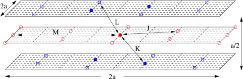
Figure 1: (Color online) Exchange interactions for CEAL, showing only the magnetic Ce atoms in three (001) planes. The structure can be thought of as consisting of two interpenetrating fcc sublattices. The Ce ${\mbox{\boldmath{$\tau$}}}_{1}$ atoms are circles (red online) and the Ce ${\mbox{\boldmath{$\tau$}}}_{2}$ atoms are squares (blue online). Filled squares represent the four Ce ${\mbox{\boldmath{$\tau$}}}_{2}$ atoms which are nearest neighbors to the Ce ${\mbox{\boldmath{$\tau$}}}_{1}$ atom at the origin, indicated by a filled circle. The exchange constants between nn’s, nnn’s, third neighbors, and fourth neighbors are $K$, $J$, $L$, and $M$, respectively.

The 4f electron of the Ce ion has quantum numbers $L=3$, $S=1/2$, and $J=|{\bf L}+{\bf S}|=L-S=5/2$, so that ${\bf S}_{\rm op}=(g_{J}-1){\bf J}$, where $g_{J}=6/7$ is the Landé $g$ factor.ASH The crystal field then splits the six states of the $J=5/2$ manifold into a ground doublet and an excited quartet state at an excitation energy of about 100K in temperature units.SPHT1 ; SPHT2 ; RES1 ; RES2 This ground doublet can be described by an effective spin operator ${\bf S}_{\rm eff}$ of magnitude 1/2 and within the doublet ${\bf J}=(5/3){\bf S}_{\rm eff}$ when admixtures from the quartet state are neglected. In that case

$${\bf S}_{\rm op}=(5/3)(g_{J}-1){\bf S}_{\rm eff}\equiv g_{0}{\bf S}_{\rm eff}\ .$$ (5)

When admixtures caused by the actual exchange field and also an applied field of 45 kOe were calculated by Barbara et al.,JS the moment was found to be somewhat larger than that zero net field, but for zero applied field we neglect this effect. Then we write the Hamiltonian in terms of effective spins 1/2 as

$${\cal H} = \sum_{{\bf R},n;{\bf R}^{\prime},n^{\prime}}J_{n,n^{\prime}}({\bf R},{\bf R}^{\prime}){\bf S}_{\rm eff}({\bf R}+{\mbox{\boldmath{$\tau$}}}_{n})\cdot{\bf S}_{\rm eff}({\bf R}^{\prime}+{\mbox{\boldmath{$\tau$}}}_{n^{\prime}})\ ,$$ (6)

where

$$J_{nn^{\prime}}({\bf R},{\bf R}^{\prime})=g_{0}^{2}J_{nn^{\prime}}^{(0)}({\bf R},{\bf R}^{\prime})\ ,$$ (7)

and we have the interactions $K$, $J$, and $M$ analogous to those in Eq. (4).

We now develop the Landau expansion for the free energy. The approach we follow is to write the trial free energy as

$$F = {\rm Tr}\left[{\mbox{\boldmath{$\rho$}}}{\cal H}+kT{\mbox{\boldmath{$\rho$}}}\ln{\mbox{\boldmath{$\rho$}}}\right]$$ (8)

where $\rho$ is the trial density matrix which is Hermitian and has unit trace. The actual free energy is the minimum of $F$ with respect to the choice of $\rho$. Mean field theory is obtained by restricting $\rho$ to be the product of single-spin density matrices, so that

$$\rho = \prod_{{\bf R},n}{\mbox{\boldmath{$\rho$}}}({\bf R},{\mbox{\boldmath{$\tau$}}}_{n})\ ,$$ (9)

where $\rho({\bf R},{\mbox{\boldmath{$\tau$}}}_{n})$ is the density matrix for the Ce spin at ${\bf R}+{\mbox{\boldmath{$\tau$}}}_{n}$. We write

$$\rho({\bf R}+{\mbox{\boldmath{$\tau$}}}_{n}) = {1\over 2}\left[1+{\bf a}({\bf R}+{\mbox{\boldmath{$\tau$}}}_{n})\cdot{\bf S}({\bf R}+{\mbox{\boldmath{$\tau$}}}_{n})\right]\ ,$$ (10)

where from now on ${\bf S}({\bf R}+{\mbox{\boldmath{$\tau$}}}_{n})$ denotes the effective spin 1/2 operator for the site in question and we identify the vector trial parameter ${\bf a}$ by relating it to the thermal expectation value of the spin as

$$\langle{\bf S}({\bf R}+{\mbox{\boldmath{$\tau$}}}_{n})\rangle = {\rm Tr}\left[{\mbox{\boldmath{$\rho$}}}({\bf R}+{\mbox{\boldmath{$\tau$}}}_{n}){\bf S}({\bf R}+{\mbox{\boldmath{$\tau$}}}_{n})\right]$$ (11)

$$= {\bf a}({\bf R}+{\mbox{\boldmath{$\tau$}}}_{n})/4\ ,$$

so that

$$\rho({\bf R}+{\mbox{\boldmath{$\tau$}}}_{n}) = {1\over 2}\left[1+4\langle{\bf S}({\bf R},{\mbox{\boldmath{$\tau$}}}_{n})\rangle{\bf S}({\bf R},{\mbox{\boldmath{$\tau$}}}_{n})\right]\ .$$ (12)

Then, one finds that

$$F = {1\over 2}\sum_{{\bf R},n;{\bf R}^{\prime},n^{\prime}}J_{n,n^{\prime}}({\bf R},{\bf R}^{\prime})\langle{\bf S}({\bf R}+{\mbox{\boldmath{$\tau$}}}_{n})\rangle\cdot\langle{\bf S}({\bf R}^{\prime}+{\mbox{\boldmath{$\tau$}}}_{n^{\prime}})\rangle$$ (13)

$$\ -TS\ ,$$

where

$$-TS = kT\sum_{{\bf R},n}{\rm Tr}\Biggl{\{}{1\over 2}\Biggl{(}1+4\langle{\bf S}({\bf R},{\mbox{\boldmath{$\tau$}}}_{n})\rangle{\bf S}({\bf R},{\mbox{\boldmath{$\tau$}}}_{n})\Biggr{)}$$ (14)

$$\ \times\ln\Biggl{(}{1\over 2}\left[1+4\langle{\bf S}({\bf R},{\mbox{\boldmath{$\tau$}}}_{n})\rangle{\bf S}({\bf R},{\mbox{\boldmath{$\tau$}}}_{n})\right]\Biggr{)}\Biggr{\}}\ ,$$

which we evaluate as

$$-TS = kT\sum_{{\bf R},n}\sum_{p=1}^{\infty}{[4\langle S({\bf R}+{\mbox{\boldmath{$\tau$}}}_{n})\rangle\cdot\langle S({\bf R}+{\mbox{\boldmath{$\tau$}}}_{n})\rangle]^{p}\over 2p(2p-1)}\ .$$ (15)

In this section we consider the term quadratic in the spin variable and in the next section we consider the quartic term in this expansion. (Higher order terms are not necessary for our analysis.)

We introduce as order parameters, the Fourier coefficients defined for $n=1,2$ by

$$\langle{\bf S}({\bf R}+{\mbox{\boldmath{$\tau$}}}_{n})\rangle = S_{n}({\bf q})e^{i{\bf q}\cdot{\bf R}}+S_{n}({\bf q})^{*}e^{-i{\bf q}\cdot{\bf R}}\ .$$ (16)

Note that the phase factor is determined by the origin of the unit cell and not by the actual location of the spin site. Any two wavevectors which differ by a linear combination of reciprocal lattice basis vectors, ${\bf G}_{n}$ are equivalent, where

$${\bf G}_{1} = 2\pi(1,1,-1)/a$$

$${\bf G}_{2} = 2\pi(1,-1,1)/a$$

$${\bf G}_{3} = 2\pi(-1,1,1)/a\ .$$ (17)

Now we write the contribution to the free energy which depends on the order parameter for some wavevector ${\bf q}$. In terms of this order parameter, the mean field free energy at quadratic order, $F_{2}$, can be written as

$$F_{2} = {1\over 2}\sum_{n,n^{\prime}}[{\mbox{\boldmath{$\chi$}}}^{-1}]_{n,n^{\prime}}S_{n}({\bf q})^{*}S_{n^{\prime}}({\bf q})\ ,$$ (18)

whereFN

$${\mbox{\boldmath{$\chi$}}}^{-1}({\bf q}) = \left[\begin{array}[]{c c }4kT+J_{11}({\bf q})&J_{12}({\bf q})\\ J_{21}({\bf q})&4kT+J_{22}({\bf q})\\ \end{array}\right]\ ,$$ (21)

where

$$J_{11}({\bf q}) = 2M(\cos q_{x}a+\cos q_{y}a+\cos q_{z}a)$$

$$\ +4J[c_{x}c_{y}+c_{x}c_{z}+c_{y}c_{z}]$$

$$= J_{22}({\bf q})$$

$$J_{12}({\bf q}) = K[1+e^{-i(q_{x}+q_{y})a/2}+e^{-i(q_{x}+q_{z})a/2}$$ (22)

$$\ +e^{-i(q_{y}+q_{z})a/2}]=J_{21}({\bf q})^{*}\ ,$$

where $c_{\alpha}=\cos(q_{\alpha}a/2)$. Omitting the factor $4kT$, the minimum eigenvalue of the ${\mbox{\boldmath{$\chi$}}}^{-1}$ matrix, which selects the wavevector, is

$$\lambda({\bf q}) = J_{11}({\bf q})-|J_{12}({\bf q})|$$ (23)

$$= 2M(2c_{x}^{2}+2c_{y}^{2}+2c_{z}^{2}-3)$$

$$\ +4J(R^{2}-1)-2|K|R\ ,$$

where

$$R = \left[1+c_{x}c_{y}+c_{x}c_{z}+c_{y}c_{z}\right]^{1/2}\ .$$ (24)

(By the square root, we always mean the positive square root.) Note that changing the signs of all the $c$’s corresponds to adding a reciprocal lattice vector to ${\bf q}$ and does not change $\lambda({\bf q})$. So solutions which differ by changing the signs of all the $c$’s are equivalent to one another. Although the minimum value of the free energy does not depend on the sign of $K$, the ratio of spin amplitudes within the unit cell does depend on this sign. To discuss the sign of $K$ it is convenient to set ${\bf q}=(1,1,1)(\pi/a)$ (which is nearly the wavevector of interest). Then if $K$ is negative (ferromagnetic), $J_{12}({\bf q})$ is negative and the minimal spin eigenvector is $(1,1)$, which indicates that the spins at ${\mbox{\boldmath{$\tau$}}}_{1}$ and ${\mbox{\boldmath{$\tau$}}}_{2}$ are parallel, as is illustrated in Fig. 2, whereas if $K$ is positive, they are antiparallel. In the former (latter) case, the other three spins of the nn tetrahedron are antiparallel (parallel) to the spin at the origin. Thus the sign of $K$ is easily related to whether the majority of the nn’s are parallel in which case $K$ is negative. Otherwise $K$ is positive. The structure determinations indicate that the correct choice is that $K$ is negative (ferromagnetic). Henceforth $K$ will be used to denote $|K|$.

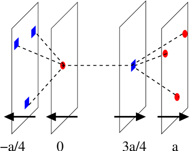
Figure 2: (Color online) Nearest neighbor interactions $K$ (indicated by dashed lines). Here we show planes perpendicular to (111), with Ce(1) sites represented by circles (red online) and Ce(2) sites represented by squares (blue online). Below each plane the value of $x+y+z$ for that plane is given. If the wavevector is assumed to be $(\pi,\pi,\pi)/a$, then all spins within a given plane are parallel to one another and if $K$ is negative (ferromagnetic), then the spin directions of each plane are as indicated by the arrows. Had $K$ been of opposite sign, then the spin directions of the Ce(2) would be reversed and an inequivalent magnetic structure would be realized.

As mentioned in the introduction, this system for $K=0$ has been comprehensively analyzed by YN. However, they seem to have overlooked an amusing limit for $K=0$. Namely, if $J=2M$ we have

$$\lambda({\bf q}) = -3J+2J(c_{x}+c_{y}+c_{z})^{2}\ .$$ (25)

For $J<0$ this is minimal for $c_{x}=c_{y}=c_{z}=\pm 1$. For $J>0$ this is minimized over the entire two dimensional manifold for which $c_{x}+c_{y}+c_{z}=0$. What this means is that for this special case, there is no wavevector selection. Such a multiphase point has been found in several models.KAG ; PYR ; NOQ As we shall see, this multiphase behavior is modified to encompass a one dimensional manifold when $K$ is small and $M<J/2$.

II.1 $J<0$

When $J<0$, then the second and third terms of Eq. (23) do not compete with one another: for a fixed value of $c_{x}^{2}+c_{y}^{2}+c_{z}^{2}$, $\lambda({\bf q})$ is minimized by maximizing $R$, which implies that $c_{x}=c_{y}=c_{z}\equiv c$, so that

$$\lambda({\bf q})=-6M+12(J+M)c^{2}-2K\sqrt{1+3c^{2}}\ .$$ (26)

The extrema must be either for $c^{2}=0$, $c^{2}=1$, or (by differentiation)

$$3c^{2} = -1+\left[{K\over 4(J+M)}\right]^{2}\ ,$$ (27)

so that, for this to apply, we must satisfy

$$4(J+M)<K<8(J+M)\ .$$ (28)

To represent the results it is convenient to set the magnitude of $J$ equal to unity, or, here, $J=-1$. In this case $M$ is restricted by

$$1+K/8<M<1+K/4\ ,$$ (29)

in which case this value of $c$ gives

Figure 3: Minimum free energy configurations for $J=-1$ as a function of $M$ and $K$. The wavevectors $\hat{\bf q}$ are indicated along with the labeling of YN for the phases.

$$\lambda({\bf q}) = -10M-4-{K^{2}\over 4(M-1)}\ .$$ (30)

When we compare this result with the value of $\lambda({\bf q})$ which we get for ${\bf q}_{\alpha}=0$ and for ${\bf q}_{\alpha}=\pi/2$, we get the phase diagram shown in Fig. 3.

II.2 $J>0$

For positive $J$ the minimization is more complicated because the second and third terms in Eq. (23) now compete. For $\lambda({\bf q})$ to be extremal, its gradient with respect to ${\bf q}$ must vanish, so that

$$0 = s_{x}\Biggl{[}-8Mc_{x}-4J(c_{y}+c_{z})+(c_{y}+c_{z})K/R\Biggr{]}\ ,$$

$$0 = s_{y}\Biggl{[}-8Mc_{y}-4J(c_{x}+c_{z})+(c_{x}+c_{z})K/R\Biggr{]}\ ,$$

$$0 = s_{z}\Biggl{[}-8Mc_{z}-4J(c_{x}+c_{y})+(c_{x}+c_{y})K/R\Biggr{]}\ .$$ (31)

There are obviously many subcases for the extrema and we will not consider equivalent solutions which correspond to changing the signs of all the $c_{\alpha}$’s or permuting their subscripts. Thus we have four cases:

$$s_{x}=s_{y}=s_{z}=0\ ,\ \ \ \ {\rm Case\ \ I}\ ,$$ (32)

$$s_{x}=s_{y}=0\ ,\ s_{z}\not=0\ ,\ \ \ \ {\rm Case\ \ II}\ ,$$ (33)

$$s_{x}=0\ ,\ \ \ \ s_{y}\not=0\ ,\ \ \ s_{z}\not=0\ ,\ \ \ \ {\rm Case\ \ III}\ ,$$ (34)

and

$$s_{x}\not=0\ ,\ \ \ s_{y}\not=0\ ,\ \ \ \ s_{z}\not=0\ ,\ \ \ \ {\rm Case\ \ IV}\ .$$ (35)

II.2.1 Case I

When $s_{x}=s_{y}=s_{z}=0$, then $c_{x}$, $c_{y}$, and $c_{z}$ can each assume the values $+1$ and $-1$. So we have

$$c_{x} = c_{y}=c_{z}=1\ ,\ \ \ \ \ {\rm Case\ \ Ia}\ ,$$

$$c_{x} = c_{y}=-c_{z}=1\ ,\ \ \ \ \ {\rm Case\ \ Ib}\ ,$$ (36)

so that

$$\lambda = 6M+12J-4K\ ,\ \ \ \ \ {\bf q}=(0,0,0)\ ,$$

$$\lambda = 6M-4J\ ,\ \ \ \ \ {\bf q}=(0,0,2\pi/a)\ .$$ (37)

Case Ia, ${\bf q}=(0,0,0)$, is the F phase of YN and Case Ib, ${\bf q}=(2\pi/a,0,0)$, the AF-I phase of YN.

II.2.2 Case II

In this case, $q_{x}$ and $q_{y}$ can independently assume the values $0$ or $2\pi/a$, so that $c_{x}$ and $c_{y}$ independently assume the values $+1$ and $-1$. Then we have

$$c_{x}=c_{y}=1\ ,\ \ \ \ {\rm Case\ \ IIa}$$ (38)

and

$$c_{x}=-c_{y}=1\ ,\ \ \ \ {\rm Case\ \ IIb}\ .$$ (39)

In Case IIa we have

$$\lambda({\bf q}) = 2M(1+2c_{z}^{2})+4J(1+2c_{x}c_{z})$$ (40)

$$\ -2K\sqrt{2+2c_{z}c_{x}}\ ,$$

so that minimization with respect to $q_{z}$ yields

$$0 = \Biggl{(}-8Mc_{z}-8Jc_{x}+{2Kc_{x}\over\sqrt{2+2c_{z}c_{x}}}\Biggr{)}s_{z}=0\ .$$ (41)

So either $s_{z}=0$ (which repeats Case I), or (since $c_{x}^{2}=1$)

$$8Mc_{z}c_{x}+8J = {2K\over\sqrt{2+2c_{z}c_{x}}}\ .$$ (42)

This gives

$$32M^{2}c_{z}^{2}+64JMc_{x}c_{z}+32{J}^{2} = {K^{2}\over 1+c_{z}c_{x}}\ .$$ (43)

For $K=0$, this gives $c_{x}c_{z}=-J/M$ and

$$\lambda({\bf q}) = 2M+4J-{4J}^{2}/M\ ,$$ (44)

which is the H$<100>$ phase of YN with wavevector $(q_{x},0,0)$. For $K=0$ this has no range of stability. For $K\not=0$ we evaluate $\lambda({\bf q})$ by solving Eq. (43) numerically.

In Case IIb we have

$$\lambda({\bf q}) = 2M(1+2c_{z}^{2})-4J\ .$$ (45)

For positive $M$ we thus have ${\bf q}=(0,2,1)\pi/a$, which is the AF-III phase of YN and

$$\lambda({\bf q}) = 2M-4J\ ,\ \ \ \ {\rm Case\ \ IIb}\ .$$ (46)

We discard the case when $M$ is negative because it repeats case Ib.

II.2.3 Case III

Here $c_{x}=\pm 1$ (we need only consider $c_{x}=+1$) and $c_{y}$ and $c_{z}$ are nonzero, determined by

$$0 = -8Mc_{y}-4J(c_{x}+c_{z})+(c_{x}+c_{z})K/R\ ,$$

$$0 = -8Mc_{z}-4J(c_{x}+c_{y})+(c_{x}+c_{y})K/R\ .$$ (47)

Subtracting and adding one equation from the other we get

$$8M(c_{y}-c_{z}) = 4J(c_{y}-c_{z})-K(c_{y}-c_{z})/R$$

$$8M(c_{y}+c_{z}) = (2c_{x}+c_{y}+c_{z})(-4J+2K/R)\ ,$$ (48)

so that

$$c_{x} = 1\ ,\ \ \ c_{y}=c_{z}\ ,\ \ \ \ \ {\rm Case\ \ IIIa}$$

$$8M(c_{y}+c_{z}) = (2+c_{y}+c_{z})(-4J+K/R)\ ,$$ (49)

$$c_{x} = 1\ ,\ \ \ 8M=4J-K/R\ ,\ \ \ \ \ {\rm Case\ \ IIIb}$$

$$8M(c_{y}+c_{z}) = (2+c_{y}+c_{z})(-4J+K/R)\ .$$ (50)

In Case IIIa we have $c_{x}=1$, $c_{y}=c_{z}$, where

$$8Mc_{y} = -4J(1+c_{y})+K\ ,$$ (51)

so that

$$c_{z}=c_{y}=(K-4J)/(8M+4J)\ ,\ \ \ \ {\rm Case\ \ IIIa}\ .$$ (52)

For this case to apply, we must satisfy the restriction

$$|K-4J|<|8M+4J|\ .$$ (53)

Then we obtain

$$\lambda({\bf q}) = -2M-2K-{(K-4J)^{2}\over 8M+4J}\ .$$ (54)

For $K=0$ this solution is H$<110>$ of YN.

In Case IIIb we have $c_{x}=1$,

$$8M=4J-K/[(1+c_{y})(1+c_{z})]^{1/2}\ ,$$ (55)

and Eq. (50) becomes

$$8M(c_{y}+c_{z}) = -8M(2+c_{y}+c_{z})\ .$$ (56)

This gives $M=0$ or

$$c_{y}+c_{z} = -1\ .$$ (57)

Since $c_{x}+c_{y}+c_{z}=0$, which will appear as Case IVc, below, we do not consider it further here.

II.2.4 Case IV

Here

$$0 = -8Mc_{x}-4J(c_{y}+c_{z})+(c_{y}+c_{z})K/R\ ,$$

$$0 = -8Mc_{y}-4J(c_{x}+c_{z})+(c_{x}+c_{z})K/R\ ,$$

$$0 = -8Mc_{z}-4J(c_{x}+c_{y})+(c_{x}+c_{y})K/R\ .$$ (58)

This set of equations is of the form

$$\left(\begin{array}[]{c c c}A&B&B\\ B&A&B\\ B&B&A\\ \end{array}\right)\left[\begin{array}[]{c}c_{x}\\ c_{y}\\ c_{z}\\ \end{array}\right]=0\ ,$$ (65)

where $A=-8M$ and $B=-4J+K/R$. Note that the eigenvalues of this matrix are $A+2B$, $A-B$, and $A-B$. The solution of this set of equations is either of type a (in which $c_{x}=c_{y}=c_{z}=0$), type b (in which the eigenvalue $A+2B$ is zero), or type c, (in which the eigenvalue $A-B$ is zero).

The solution of type a is case IVa, with

$$c_{x}=c_{y}=c_{z}=0\ ,\ \ \ \ \lambda({\bf q})=-6M-2K\ .$$ (66)

For $K=0$, this is AF-II of YN.

The solution to Eq. (65) of type b is Case IVb with

$$(c_{x},c_{y},c_{z}) = (c,c,c)\ ,\ \ \ \ A+2B=0\ .$$ (67)

Setting $A+2B=0$ leads to

$$c = \left[{1\over 3}\right]^{1/2}\left[\left({K\over 4(J+M)}\right)^{2}-1\right]^{1/2}\ ,$$ (68)

and we have the constraint

$$1<{K\over 4(J+M)}<2\ ,$$ (69)

and therefore this regime does not appear in the limit studied by YN. Then

$$\lambda({\bf q}) = -10M-4J-{K^{2}\over 4(J+M)}\ .$$ (70)

The solution to Eq. (65) of type c requires $A-B=0$ and the solution must be a linear combination of the two associated eigenvectors. So we introduce Potts-like variablesPOTTS

$$(c_{x},c_{y},c_{z}) = \left(-{\alpha\over\sqrt{2}}-{\beta\over\sqrt{6}}\ ,{\alpha\over\sqrt{2}}-{\beta\over\sqrt{6}}\ ,{2\beta\over\sqrt{6}}\right)\ .$$ (71)

Note that we have

$$c_{x}^{2}+c_{y}^{2}+c_{z}^{2} = \alpha^{2}+\beta^{2}$$ (72)

and

$$c_{x}c_{y}+(c_{x}+c_{y})c_{z} = -{1\over 2}(\alpha^{2}+\beta^{2})\ .$$ (73)

The equation $A-B=0$ is

$$0 = 4J-8M-{K\over\sqrt{1-(\alpha^{2}+\beta^{2})/2}}\ .$$ (74)

If we write

$$4J=8M+\xi K\ ,$$ (75)

where $\xi$ can not be negative, then

$$\alpha^{2}+\beta^{2}=2-2\xi^{-2}\equiv X^{2}\ .$$ (76)

This indicates that $\xi>1$ or

$$0<{K\over 4J-8M}<1\ .$$ (77)

Thus we set

$$\alpha = X\cos\theta\ ,\ \ \ \ \beta=X\sin\theta\ ,$$ (78)

where the restriction on $\theta$ will be discussed. These evaluations give

$$X^{2}=2-2\left[{K\over 4J-8M}\right]^{2}\equiv 2-2(K/K_{c})^{2}\ ,$$ (79)

so that

$$\lambda({\bf q}) = 2M-4J-{K^{2}\over 4J-8M}\ ,\ \ \ \ {\rm Case\ \ IVc}$$ (80)

and we have the constraint of Eq. (77). Then, Eq. (71) gives

$${\bf c} \equiv (c_{x},c_{y},c_{z})$$ (81)

$$= {2X\over\sqrt{6}}[\sin\left(\theta-2\pi/3),\sin(\theta+2\pi/3),\sin\theta\right]\ .$$

Note that $\theta$ is arbitrary, so this minimum is realized along a curve in wavevector space. Equation (76) shows that $X\leq\sqrt{2}$. As long as $X$ is less than $\sqrt{6}/2$ (i. e. $K_{c}>K>K_{c}/2$), all values of $\theta$ are acceptable. If $X$ lies between $\sqrt{6}/2$ and $\sqrt{2}$ (i. e. $0<K<K_{c}$), then values of $\theta$ symmetric around $\theta=0$ (and also around $\theta=k\pi/3$,

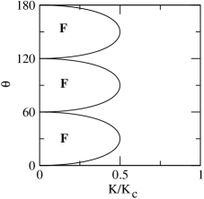
Figure 4: Allowed and forbidden (indicated by an F) regions $\theta$ (in degrees) versus $K/K_{c}$, where $K_{c}=4J-8M$.

where $k$ is an integer) in which none of the $c$’s exceed one in magnitude are allowed. The allowed region, $-\theta_{c}<\theta<\theta_{c}$, is determined by the condition

$$(2/\sqrt{6})X\sin(\theta_{c}+\pi/3)=1\ .$$ (82)

The allowed regions of $\theta$ are illustrated in the Fig. 4. We will call this phase the M’ phase.

Table 1: Free energies of the various states.

Case	Energy	$\hat{\bf q}$	For	YN Casea
Ia	$6M+12J-4K$	$(0,0,0)$	Any	F
Ib	$6M-4J$	$(1,0,0)$	Any	AF-I
IIa	Complexb	$(q_{x},0,0)$	$|J/M|<1^{\rm c}$	H$<$100$>$
IIb	$2M-4J$	(0,1,1/2)	Any	AF-III
IIIa	$-2M-2K-{(K-4J)^{2}\over 8M+4J}$	$(0,q_{y},q_{y})$	$\left|{K-4J)\over(8M+4J)}\right|<1$	H$<$110$>$
IVa	$-6M-2K$	$(1/2,1/2,1/2)$	Any	AF-II
IVb	$-10M-4J-{K^{2}\over 4(J+M)}$	$(q_{x},q_{x},q_{x})$	${1\over 2}<{4(J+M)\over K}<1$
IVc	$2M-4J-{K^{2}\over 4J-8M}$	$\left({1\over 2}-\delta,{1\over 2}+\delta,{1\over 2}\right)^{\rm d}$	$K<4J-8M$

a For $K=0$.

b For $K=0$, the energy is $4J+2M-4J^{2}/M$.

c This restriction is only for $K=0$.

d For $K=0$ we have a two-parameter multiphase: $c_{x}+c_{y}+c_{z}=0$. For $K\not=0$, the single parameter $\theta$ of Eq. (81) is not fixed.

Although $\theta$ is arbitrary, to get the wavevector seen by experiment, we want to have

$${\bf q}a=(\pi-2\pi\delta\ ,\pi+2\pi\delta,\pi)\ ,$$ (83)

so that

$$c_{x} = \cos(\pi/2-\pi\delta)=\sin(\pi\delta)\ ,$$

$$c_{y} = \cos(\pi/2+\pi\delta)=-\sin(\pi\delta)\ ,$$

$$c_{z} = \cos(\pi/2)=0\ .$$ (84)

This corresponds to $\theta=\pi$ in Eq. (81), so that

$$\sin(\pi\delta) = (2X/\sqrt{6})\sin(\pi/3)=(X/\sqrt{2})$$ (85)

$$= \left[1-\left({K\over 4J-8M}\right)^{2}\right]^{1/2}=\left[1-\left({K\over K_{c}}\right)^{2}\right]^{1/2}\ .$$

Presumably fluctuation effects or further neighbor interactions select $\theta=\pi$ from the degenerate manifold of all $\theta$ which minimize $\lambda({\bf q})$ and we will consider the second mechanism in the Sec. III.

II.2.5 Comparison of Extrema

To find the global minimum of the eigenvalue, we must compare the values of the functions at the above extrema. For this purpose we summarize the results in Table 1.

Since Case IIa is hard to analyze analytically, we had recourse to a computer program to compare the various local extrema and select the global minimum. Having done that, we checked some of the results analytically with the result shown in Fig. 5. It is interesting that turning on $K$ immediately renders the AF-I and AF-III phase unstable. Note also that the M’ phase (which is the one we want for CEAL) does occur for $K$ as large as $4J$ and $M$ being quite small. This agrees with the idea that the interactions decrease with increasing separation so that $|K|>|J|>M$.

Finally, we remark that the model with only $K$ and $J$ nonzero lacks wavevector selection for $K<8J$ because $\lambda({\bf q})$ only depends on $R$. So this means that $c_{x}$, $c_{y}$, and $c_{z}$ range over a two parameter manifold of fixed $R$.

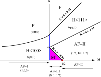
Figure 5: (Color online) Minimum free energy configurations for $J=1$, as a function of $M$ and $K$. The components of the wavevector (in units of $2\pi/a$) are the triad of numbers in parentheses. The point $K=0$, $M=1/2$ (filled circle, online red) is a two-parameter multiphase point where all states satisfying $c_{x}+c_{y}+c_{z}=0$ have minimal free energy. For $K\not=0$, the region (online magenta) labeled $M^{\prime}$ is the multiphase region in which the single parameter $\theta$ can be chosen as in Fig. 4. The line segment (online blue) $M=0$, $K<8$ is a multiphase region in which only the value of $R=K/4$ [see Eq. (23) is fixed. The phase transitions are continuous except for those at $M=0$. As soon as $K$ is nonzero, the AF-I phase gives way to the H$<110>$ phase having small $q$. and the AF-III phase gives way to the M’ phase which has wavevector within the allowed range of $\theta$ of Eq. (81).

III FURTHER NEIGHBOR INTERACTIONS

In this section we consider the effect of third- and further-than-fourth- neighbor interactions.

III.1 A “4$J$” MODEL

We start by including third-neighbor (tnn) interaction coefficients $L$, as shown in Fig. 1, so that we have a $4J$ model. This interaction occurs at separations equivalent to $(3,1,\overline{1})a/4$. Including them does not affect $J_{11}({\bf q})$ or $J_{22}({\bf q})$ but now

$$J_{12}({\bf q}) = J_{21}({\bf q})^{*}=e^{-ia(k_{x}+k_{y}+k_{z})/4}[K\Phi+L\Psi]$$ (86)

where $\Phi$ is as before, but now

$$\Psi = e(31\overline{1})+e(3\overline{1}1)+e(\overline{3}11)+e(\overline{3}\overline{1}\overline{1})+{\cal P}\ ,$$ (87)

where $e(lmn)=\exp[i(lk_{x}+mk_{y}+nk_{z})a/4]$ and ${\cal P}$ indicates inclusion of the permutations ${\cal P}=c_{x}\rightarrow c_{y}\rightarrow c_{z}\rightarrow c_{x}$. Then

$$\lambda({\bf k}) = 4J(c_{x}c_{y}+c_{y}c_{z}+c_{z}c_{x})-6M$$ (88)

$$\ +4M(c_{x}^{2}+c_{y}^{2}+c_{z}^{2})-2KR\ ,$$

where now

$$R^{2} = [1+A]+(L/K)\Delta+(L/K)^{2}\Pi\ ,$$ (89)

with

$$\Delta = {1\over 4}\left[\Phi^{*}\Psi+\Phi\Psi^{*}\right]=-6+2A+4B+4C$$ (90)

$$\Pi = {1\over 4}\Psi^{*}\Psi$$ (91)

$$= 9-7A-8B+8C+4D+8E-4F\ .$$

Also

$$A = c_{x}c_{y}+c_{x}c_{z}+c_{y}c_{z}$$

$$B = c_{x}^{2}+c_{y}^{2}+c_{z}^{2}$$

$$C = (c_{x}+c_{y}+c_{z})c_{x}c_{y}c_{z}$$

$$D = (c_{x}+c_{y}+c_{z})(c_{x}^{3}+c_{y}^{3}+c_{z}^{3})$$

$$E = (c_{x}^{2}c_{y}^{2}+c_{y}^{2}c_{z}^{2}+c_{z}^{2}c_{x}^{2})$$

$$F = (c_{x}^{4}+c_{y}^{4}+c_{z}^{4})\ .$$ (92)

We will not pursue the analysis to the same level as for the 3J model. Here we will show that for an interior point in $c_{x},c_{y},c_{z}$ space (i. e. when all these variables are less than 1 in absolute value), there is no extremum of $\lambda({\bf q})$ for which all the $c$’s are different from one another. (Thus this model can not give the state of the type ${\bf c}=(c,-c,0)$, observed for CEAL.CEAL5 ; CEAL6 ) For this analysis we consider the equations $\partial\lambda({\bf q})/\partial c_{\alpha}=0$ under the assumption that all the $c$’s are different from one another. For $\alpha=x$ this derivative condition is

$$0 = 4J(c_{y}+c_{z})+8Mc_{x}-{1\over R}\Biggl{[}K(c_{y}+c_{z})$$ (93)

$$+ L(2c_{x}+2c_{y}+8c_{x}+4c_{y}c_{z}(c_{x}+c_{y}+c_{z})+4c_{x}c_{y}c_{z}\Biggr{]}$$

$$+ (L^{2}/K)\Biggl{[}-16c_{x}-7c_{y}-7c_{y}-56c_{x}^{3}+16c_{x}c_{y}^{2}+16c_{x}c_{z}^{2}$$

$$+ (12c_{x}^{2}+8c_{y}c_{z})(c_{x}+c_{y}+c_{z})+4c_{x}^{3}+8c_{x}c_{y}c_{z}\Biggr{]}\ .$$

We now subtract from this equation that which one gets by the permutation ${\cal P}$ and divide the result by $c_{x}-c_{y}$, a quantity which, by assumption, is nonzero. Thereby we obtain

$$0 = -4J+8M-{1\over R}\Biggl{(}-K+L[6-4c_{z}(c_{x}+c_{y}+c_{z})]$$ (94)

$$\ +(L^{2}/K)[-9-56(c_{x}^{2}+c_{x}c_{y}+c_{y}^{2})-16c_{x}c_{y}$$

$$\ +16c_{z}^{2}+12(c_{x}+c_{y})(c_{x}+c_{y}+c_{z})$$

$$-8c_{z}(c_{x}+c_{y}+c_{z})+4(c_{x}^{2}+c_{y}^{2}+c_{z}^{2})\Biggr{)}\ .$$

Now, again subtract from this equation that which one gets by the permutation ${\cal P}$ and divide the result by $c_{x}-c_{z}$, a quantity which, by assumption, is nonzero. Thereby we get

$$0 = L(c_{x}+c_{y}+c_{z})-48(L^{2}/K)(c_{x}+c_{y}+c_{z})$$ (95)

which indicates that $c_{x}+c_{y}+c_{z}=0$. Therefore we introduce the Potts representation in the form

$$c_{x}={\xi\over\sqrt{3}}+{X[\sin\theta+\sqrt{3}\cos\theta]\over\sqrt{6}}$$

$$c_{y}={\xi\over\sqrt{3}}+{X[\sin\theta-\sqrt{3}\cos\theta]\over\sqrt{6}}$$

$$c_{z}={\xi\over\sqrt{3}}-{2X\sin\theta\over\sqrt{6}}\ .$$ (96)

If there is an extremum for which all the $c$’s are different from one another, the calculation we have just done shows that it must occur for $\xi=0$. Rather than further analyze the derivative conditions, it is instructive to consider $\lambda({\bf q})$ in terms of these Potts variables. We have

$$A = \xi^{2}-{1\over 2}X^{2}\ ,$$

$$B = \xi^{2}+X^{2}\ ,$$

$$C = {\xi^{4}\over 3}-{1\over 2}\xi^{2}X^{2}-{1\over 3\sqrt{2}}\xi X^{3}\sin(3\theta)\ ,$$

$$D = \xi^{4}+3\xi^{2}X^{2}-{1\over\sqrt{2}}\xi X^{3}\sin(3\theta)\ ,$$

$$E = {\xi^{4}\over 3}+{1\over 4}X^{4}+{\sqrt{2}\over 3}\xi X^{3}\sin(3\theta)\ ,$$

$$F = {\xi^{4}\over 3}+2\xi^{2}X^{2}+{1\over 2}X^{4}-{2\sqrt{2}\over 3}\xi X^{3}\sin(3\theta)\ .$$ (97)

Thus

$$\Delta = -6+6\xi^{2}+3X^{2}+{4\over 3}\xi^{4}-2\xi^{2}X^{2}-{2\sqrt{2}\over 3}\xi X^{3}\sin(3\theta)\ ,$$

$$\Pi = 9-15\xi^{2}-{9\over 2}X^{2}+8\xi^{4}+2\sqrt{2}\xi X^{3}\sin(3\theta)\ .$$ (98)

The important point is that, correct to leading order in $L/K$ we have

$$R=f(\xi^{2},X^{2})-{\sqrt{2}\over 3}(L/K)\xi X^{3}\sin(3\theta)\ ,$$ (99)

and therefore a contribution to $\lambda({\bf q})$ of

$$\delta\lambda({\bf q})\sim{2\sqrt{2}\over 3}L\xi X^{3}\sin(3\theta)\ .$$ (100)

Thus the fact that $L$ is nonzero leads to a nonzero term in $\lambda({\bf q})$ which is linear in $\xi$ and renders the manifold $c_{x}+c_{y}+c_{z}=0$ unstable. Since the quadratic term in $\xi$ is of the form

$$\lambda({\bf q})\sim 1/2\chi_{\xi}^{-1}\xi^{2}$$ (101)

with $\chi_{\epsilon}^{-1}\approx 8J-2K$, we see that, when a minimization with respect to $\xi$ is performed, one has

$$\xi = -{2\sqrt{2}\chi_{\xi}\over 3}LX^{3}\sin(3\theta)$$ (102)

and now we generate the following term in $\lambda({\bf q})$ which depends on $\theta$:

$$\lambda({\bf q}) = f(X^{2})-{4\chi_{\xi}\over 9}L^{2}X^{6}\sin^{2}(3\theta)\ .$$ (103)

When $L$ is nonzero, it generates a nonzero value of $\xi$, i. e. it would take the extremum slightly out of the plane $c_{x}+c_{y}+c_{z}=0$. But, according to Eq. (95), the minimum with the $c_{\alpha}$’s being unequal, can only occur in the plane $c_{x}+c_{y}+c_{z}=0$. So, if a minimum can not occur in this plane, it can not occur anywhere in the interior of ${\bf c}$ space. In addition, even if a small displacement out of this plane were allowed (and it would not be totally unacceptable in view of the experimental data if $\xi$ were small enough), the $\theta$-dependent term in Eq. (103) favors $\theta=\pi/2$, which would give a wavevector of the form $a{\bf q}/(2\pi)=(1/2-\delta,1/2-\delta,1/2+2\delta)$, which the experimental data do not permit. Within the 4J model this problem can not overcome because the sign of this anisotropy in $\theta$ can not be adjusted (it enters in terms of positive definite quantities).

III.2 STILL FURTHER NEIGHBOR INTERACTIONS

The preceding calculation, although unsuccessful in producing an explanation of the data, is nevertheless instructive. It indicates that we need to focus on the sixth order anisotropy (in c space) coming from further neighbor interactions. This requires a term involving six powers of the $c$’s. The leading candidate for such a term is the exchange interaction at the separation $(a,a,a)$. From these eight equivalent neighbors, with exchange constant $Q$, one finds the additional contribution to $J_{nn}({\bf q})$ to be

$$\delta J_{nn}({\bf q}) = 8Q\cos(aq_{x})\cos(aq_{y})\cos(aq_{z})$$ (104)

$$= 8Q(2c_{x}^{2}-1)(2c_{y}^{2}-1)(2c_{z}^{2}-1)\ ,$$

which leads to an additional term in $\lambda({\bf q})$ whose dependence on $\theta$ is of the form

$$\delta\lambda({\bf q}) = 64Qc_{x}^{2}c_{y}^{2}c_{z}^{2}$$ (105)

$$= Q\Biggl{(}{8\xi^{3}\over 3\sqrt{3}}-{8\xi X^{2}\over 2\sqrt{3}}-{8\over 3\sqrt{6}}X^{3}\sin(3\theta)\Biggr{)}^{2}$$

$$\sim {32\over 27}QX^{6}\sin^{2}(3\theta)\ .$$

(Here we dropped the less significant terms proportional to $\sin(3\theta)$.) The sign of this term is adjustable and it will have the opposite sign from the anisotropy due to $L$ if $Q$ is positive (antiferromagnetic). It will then favor $\theta=n\pi/3$ in Eq. (96) and if this anisotropy dominates, then the wavevector will be of the desired form: $a{\bf q}/(2\pi)=(1/2-\delta,1/2+\delta,1/2)$.

If we only consider $L$ and $Q$, then the condition that this anisotropy have the correct sign to explain the wavevectors of CEAL is that

$$Q>(3/8)\chi_{\xi}L^{2}\ .$$ (106)

Since the model now has four parameters, we did not pursue a definitive numerical analysis of the minima. However, to corroborate this argument is sound, we give in Table 2 some values of the input parameters which give ${\bf c}=(c,-c,0)$, for $c$ equal to the experimental value $c=\sin\pi\delta=0.338$ for $\delta=0.11$.CEAL5 ; CEAL6 This table illustrates the phase transition in the anisotropy in ${\bf c}$-space which takes place for small $Q$ at a value close to that predicted by the approximate bound of Eq. (106). Note that for small values of $L$ and $Q$, the values of the other parameters which give the desired form of ${\bf c}$ can not be far from the region M’ of Fig. 5.

Table 2: Values of the exchange integrals (for $J=1$) which give values of ${\bf c}$ close to the observed values of ${\bf c}$. Note that a small change in $Q$ causes the anisotropy in ${\bf c}$-space to change.

$|K|$	$L$	$M$	$Q$	$c_{x}$	$c_{y}$	$c_{z}$
$3.50^{\rm a}$	$-0.04$	$0.016$	$0.0010$	$-0.339$	$0.001$	$0.338$
3.50	$-0.04$	$0.016$	$-0.0010$	$-0.425$	$0.215$	$0.215$
3.50	$-0.04$	$0.017$	$0.0010$	$-0.333$	$0.000$	$0.333$
3.50	$-0.03$	$0.016$	$0.0010$	$-0.360$	$0.000$	$0.360$
$3.50^{\rm a}$	$-0.08$	$-0.012$	$0.0050$	$-0.337$	$0.000$	$0.337$
3.00	$0.08$	$0.131$	$0.0010$	$-0.344$	$0.022$	$0.321$
3.00	$0.08$	$0.131$	$0.0006$	$-0.358$	$0.033$	$0.324$
3.00	$0.08$	$0.131$	$0.0000$	$-0.410$	$0.203$	$0.206$
$3.00^{\rm a}$	$0.00$	$0.102$	$0.0001$	$-0.333$	$0.000$	$0.333$
$3.00^{\rm a}$	$0.04$	$0.116$	$0.0004$	$-0.340$	$0.000$	$0.340$
$3.00^{\rm a}$	$-0.04$	$0.085$	$0.0003$	$-0.336$	$0.000$	$0.336$
$3.00^{\rm a}$	$-0.08$	$0.066$	$0.0012$	$-0.338$	$0.000$	$0.338$
$3.00^{\rm a}$	$-0.12$	$0.046$	$0.0025$	$-0.338$	$0.000$	$0.338$
2.50	$-0.08$	$0.160$	$0.0008$	$0.000$	$0.000$	$0.000$
$2.50^{\rm a}$	$-0.08$	$0.134$	$0.0008$	$-0.335$	$0.000$	$0.335$
$2.50^{\rm a}$	$-0.12$	$0.114$	$0.0020$	$-0.338$	$0.000$	$0.338$
2.50	$-0.12$	$0.150$	$0.0020$	$0.000$	$0.000$	$0.000$
$2.00^{\rm a}$	$-0.12$	$0.180$	$0.0020$	$-0.342$	$0.001$	$0.341$
$2.00^{\rm a}$	$-0.08$	$0.200$	$0.0008$	$-0.338$	$0.000$	$0.338$
$1.50^{\rm a}$	$-0.08$	$0.268$	$0.0004$	$-0.334$	$0.000$	$0.334$
$1.50^{\rm a}$	$-0.12$	$0.247$	$0.0020$	$-0.336$	$0.001$	$0.335$

a) For this line of parameters, adding $-0.002$ to $Q$ takes ${\bf c}$ from the $(c,-c,0)$ phase into the $(2c,-c,-c)$ phase (e. g. see the first and second lines of this table).

III.3 EXPERIMENTAL DETERMINATION OF PARAMETERS

In principle we can fix the magnitudes of the dominant exchange integrals by relating them to several experimentally observed quantities. These quantities include the value of the ordering temperature, $T_{c}$, the Curie-Weiss temperature, $\Theta_{\rm C-W}$, for the susceptibility

$$\chi\sim C/(T-\Theta_{\rm C-W})\ ,$$ (107)

and the high-temperature (compared to $T_{c}$) specific heat.SPHT1 ; SPHT2 We consider these in turn and will obtain an estimate for the largest exchange constants $J$ and $K$ (which here we denote $K_{0}$ to avoid confusion with the symbol for Kelvin temperature units.) Crudely we estimate that due to fluctuations not included within mean field theory the actual ordering temperature, $3.8$K, is about $2T_{\rm MF}/3$, so that $T_{\rm MF}\approx 6$K. From Eq. (21) we deduce that (neglecting $L$ and $Q$)

$$24{\rm K} = 4T_{\rm MF}=-\lambda({\bf q})/k$$ (108)

$$= (-1.88K_{0}+0.46J+5.10M)/k\ ,$$

where we took $K_{0}$ to be negative (bearing in mind the discussion of Fig. 2), and we evaluated the constants for ${\bf c}=(0.338,-0.338,0)$. If we only take into account the interaction $K_{0}$, we get $K_{0}/k=-13$ K. To see what zero-temperature splitting, $\Delta E$, of the doublet this implies, note that both $T_{\rm MF}$ and $\Delta E$ are proportional to $J({\bf q})$, the Fourier transform of the exchange integral. This type of relation leads to

$$\Delta E={3\over S+1}kT_{\rm MF}=2kT_{\rm MF}\ ,$$ (109)

so that $\Delta E/k=12$K. This nearly agrees with the result $\Delta E/k\approx 15$K, given by Boucherle and Schweizer.PHYSICA

Next we consider the Curie-Weiss temperature. This is a particularly good quantity to compare to calculations because, being the first nontrivial term in the high temperature expansion of the uniform susceptibility, it is not subject to fluctuation corrections. In Appendix B we give a generalization of Eq. (107) which takes the crystal field splitting into account. There we show that the Curie-Weiss intercept extrapolated from values of the susceptibility $\chi$ at infinite temperature is related to the exchange constants via

$$-\sum_{j}J_{ij}/k = (20/21)\Theta_{\rm C-W}\ .$$ (110)

Following reference CURIE1, we set the Curie-Weiss intercept equal to -33K. But, as shown in Appendix B, to get this value when an is made from data at $T<300$K (rather than from infinite temperature), it is necessary to take

$$-28.5{\rm K} = \sum_{j}J_{ij}/k\approx(4K_{0}+12J)/k\ .$$ (111)

If we neglect $M$, then Eqs. (108) and (111) lead to the determination

$$K_{0}/k = -11.3{\rm K}\ ,\ \ \ J/k=6.1{\rm K}\ .$$ (112)

The value of $K_{0}$ is fixed to within about 10% by Eq. (108), but the value of $J$ is subject to larger (say 20%) uncertainty. A question which we can not settle is whether it is justified to rely on a pure Heisenberg model to interpret that Curie-Weiss susceptibility. Attributing contributions to the susceptibility to the conduction electrons or to the diamagnetism of core electrons would somewhat modify our estimates.

The magnetic specific heat $C$ for a system governed by the spin Hamiltonian ${\cal H}$ gives rise to the limiting value $CT^{2}/k$ at infinite temperature given by

$$CT^{2}/k = {{\rm Tr}{\cal H}^{2}\over{\rm Tr}1}={1\over 2}\sum_{i,j}{{\rm Tr}J_{ij}^{2}({\bf S}_{i}\cdot{\bf S}_{j})^{2}\over{\rm Tr}1}$$ (113)

$$= {1\over 6}\sum_{i,j}J_{ij}^{2}[S(S+1)]^{2}={3N\over 32}\sum_{j}J_{ij}^{2}$$

$$= {3N\over 32}[4K_{0}^{2}+12J^{2}+6M^{2}+12L^{2}]\ ,$$

where $N$ is the total number of Ce ions. This quantity might not be easy to determine experimentally because it requires separating off from the total measured specific heat (in the temperature range, say, $10{\rm K}<T<20{\rm K}$), the amount attributed to the lattice and conduction electrons.

Finally, we should mention that the interactions we determine are those renormalized by virtual excitation to excited crystal field states. Normally, one might ignore such effects. However, as we show in Appendix C, the contribution to $J$ from these virtual processes is of the same order as we have just determined by our fit to experiment. These virtual process also imply that long range interactions must be present even if one does not invoke RKKY interactions. So our appeal to the $Q$ interaction [at separation $(a,a,a)$] is not unreasonable.

III.4 APPLICATION TO TmS

At this point we recall that wavevector selection in TmS is of the same form as for CEAL [see Eq. (1)], but with $\delta=0.075$.TMS2 In TmS the Tm spins form an fcc lattice, so the lattice geometry is not the same as for CEAL and for TmS the interactions $K$ and $L$ do not occur. However, TmS is similar to CEAL in that one can imagine the dominant exchange interactions limiting one to be close to the subspace $c_{x}+c_{y}+c_{z}=0$, in which case a major concern is to have the anisotropy in wavevector space, as in Eq. (105), so that the incommensuration is of the form ${\bf c}=(\delta,-\delta,0)$ rather than ${\bf c}=(\delta,\delta,-2\delta)$. We illustrate this analogy by a brief numerical survey of the selected wavevector as a function of the interaction $Q$ (for separation $(1,1,1)$) as in Eq. (104). The result in Table 3 shows again the effect of this term on the anisotropy in wavevector space which can be invoked to explain the pattern of incommensuration similar to that of CEAL. In addition, we mention that like CEAL, no higher harmonics, especially at wavevector $3{\bf q}$ were detected.TMS2 We propose that, as we show in the next section, this could be understood if the magnetic structure of TmS were to consist of the superposition of exactly two wavevectors, as is the case for CEAL.CEAL5 ; CEAL6

Table 3: Wavevectors at which $\lambda({\bf q})$ is minimal for values of the exchange interactions (in arbitrary units) for the listed separations (in units of the lattice constant) on an fcc lattice as a function of the $(1,1,1)$ interaction analogous to $Q$ of Eq. (104). All interactions are positive (antiferromagnetic).

Exchange Interactions					$\cos(q_{\alpha}a/2)$
(${1\over 2},{1\over 2},0$)	(1,0,0)	(${1\over 2},{1\over 2},1$)	(1,1,0)	(1,1,1)	$c_{x}$	$c_{y}$	$c_{z}$
2.000	1.000	0.150	0.044	0.003	-0.304	0.000	0.304
2.000	1.000	0.150	0.044	0.002	-0.334	-0.002	0.336
2.000	1.000	0.150	0.044	0.001	-0.412	0.150	0.264
2.000	1.000	0.150	0.044	0.000	-0.444	0.224	0.224

IV QUARTIC TERMS IN THE LANDAU FREE ENERGY

In this section we analyze the quartic terms in the Landau free energy in order to investigate the coupling between wavevectors in the star of ${\bf q}$. Before starting this complicated calculation, we describe briefly the physical effects we will address. As the temperature is lowered in the ordered phase, the effect of the quartic terms in the Landau free energy, which is to favor fixed length spins, progressively increases. This phenomenon is particularly significant for incommensurate systems. For many systems having uniaxial anisotropy, order first occurs in which the spins are aligned along the easy axis with sinusoidally modulated amplitude.Nagamiya In that case, when the temperature is sufficiently lowered so that the fourth order terms become important, the fixed length constraint causes the appearance of transverse spin order, which implies a phase transition,Nagamiya and Ni₃V₂O₈ is a recent example of this phenomenon.NVO As we shall see, in CEAL the fixed length constraint favors the simultaneous appearance of incommensurate structures at the two wavevectors which combine properly to minimize fluctuations in the spin lengths. To show this analytically is algebraically quite complicated, as will become apparent. (If we only wished to show that the double q state was favored relative to the single q state, as was done in Ref. dq2, , the calculation would be much simpler. However, our aim was to show that the double q state was favored over all other possibilities.)

In the preceding section we discussed wavevector selection within a model of isotropic exchange interactions. This model is somewhat misleading in that it has much higher symmetry than that required by crystal symmetry. When more general interactions are present, the eigenvector of the quadratic free energy matrix associated with the eigenvalue which first becomes nonpositive as the temperature is lowered determines the form and symmetry of the long range order. This critical eigenvector must transform according to an irreducible representation (irrep) of the symmetry group of the crystal, as is discussed recently by one of us.JS1 This discussion tacitly assumes the impossibility of accidental degeneracy wherein two or more irreps having different symmetry could simultaneously condense. Accordingly we expect that

$${\bf S}^{\tau}_{\alpha}({\bf R}) = \sum_{n=1}^{12}S_{\alpha}^{\tau}({\bf q}_{n})e^{i{\bf q}_{n}\cdot{\bf R}}\ +{\rm c.\ c.}\ ,$$ (114)

where ${\bf S}^{\tau}({\bf R})$ is the spin vector at the $\tau$th site in the unit cell at ${\bf R}$, c. c. indicates the complex conjugate of the preceding terms, and the sum is over the 12 wavevectors ${\bf q}_{i}$ which, together with $-{\bf q}_{i}$, comprise the star of ${\bf q}$. For some purposes it is convenient to divide the ${\bf q}_{i}$’s into three classes ${\bf Q}^{\mu}_{\alpha}$ for $\mu=\alpha,\beta,\gamma$ such that for $n=1,2,3,4$

$${\bf q}_{n} = {\bf Q}^{\alpha}_{n}\ ,\ {\bf q}_{n+4}={\bf Q}^{\beta}_{n}\ ,\ {\bf q}_{n+8}={\bf Q}^{\gamma}_{n}\ ,$$ (115)

where the ${\bf Q}$’s are listed in Tables 4, 5, and 6. Near the ordering temperature $S_{\alpha}^{\tau}({\bf q}_{i})$ can be written as a temperature-dependent complex-valued amplitude $x_{i}(T)$ times the critical eigenvector $m_{\alpha}^{\tau}({\bf q}_{i})$ normalized by $\sum_{\alpha n}|m_{\alpha}^{{\mbox{\boldmath{$\tau$}}}_{n}}|^{2}=1$. Then

$${\bf S}^{\tau}_{\alpha}({\bf R}) = \sum_{n=1}^{12}x_{n}{\bf m}^{\tau}({\bf q}_{n})e^{i{\bf q}_{n}\cdot{\bf R}}\ +{\rm c.\ c.}$$ (116)

Thus the $x_{n}$’s are the complex-valued order parameters of this system. The result of representation theory for CEAL, given in Ref. JS2, , is that for the wavevector ${\bf q}_{1}=(1/2-\delta,1/2+\delta,1/2)(2\pi/a)$, the critical eigenvector, which gives the spin components of the two sites in the unit cell for the irrep which experimentsCEAL1 ; CEAL2 ; CEAL5 ; CEAL6 have shown to be the active one, is of the form

$${\bf m}^{{\mbox{\boldmath{$\tau$}}}_{1}}({\bf q}_{1}) = (\alpha e^{i\phi},\alpha e^{-i\phi}\ ,\beta)\ ,$$

$${\bf m}^{{\mbox{\boldmath{$\tau$}}}_{2}}({\bf q}_{1}) = (-\alpha e^{-i\phi},-\alpha e^{i\phi}\ ,\beta)\ ,$$ (117)

where the real-valued parameters $\alpha$, $\beta$, and $\phi$ depend on the interactions but can be determined from experimental data. The next step in this calculation is to use crystal symmetry to relate the eigenvectors for the other wavevectors in the star of ${\bf q}$ to that given in Eq. (117). This is done in the Appendix and the results are listed in Tables 4, 5, and 6.

Table 4: Wavefunctions for the ${\bf Q}^{\alpha}$ wavevectors.^(a)

$n$	${\bf Q}^{\alpha}_{n}$			${\bf m}^{1}({\bf Q}^{\alpha}_{n})$			${\bf m}^{2}({\bf Q}^{\alpha}_{n})$
1	${1\over 2}-\delta$	${1\over 2}+\delta$	${1\over 2}$	$\alpha e^{i\phi}$	$\alpha e^{-i\phi}$	$\beta$	$-\alpha e^{-i\phi}$	$-\alpha e^{i\phi}$	$-\beta$
2	${1\over 2}-\delta$	${1\over 2}+\delta$	$-{1\over 2}$	$\alpha e^{-i\phi}$	$\alpha e^{i\phi}$	$-\beta$	$\alpha e^{i\phi}$	$\alpha e^{-i\phi}$	$-\beta$
3	${1\over 2}-\delta$	$-{1\over 2}-\delta$	${1\over 2}$	$-\alpha e^{i(\pi\delta-\phi)}$	$\alpha e^{i(\pi\delta+\phi)}$	$-\beta e^{i\pi\delta}$	$-\alpha e^{i\phi}$	$\alpha e^{-i\phi}$	$-\beta$
4	${1\over 2}-\delta$	$-{1\over 2}-\delta$	$-{1\over 2}$	$-\alpha e^{i(\pi\delta+\phi)}$	$\alpha e^{i(\pi\delta-\phi)}$	$\beta e^{i\pi\delta}$	$-\alpha e^{-i\phi}$	$\alpha e^{i\phi}$	$\beta$

a) Wavevectors are given in units of $2\pi/a$.

Table 5: Wavefunctions for the ${\bf Q}^{\beta}$ wavevectors.^(a)

$n$	${\bf Q}^{\beta}_{n}$			${\bf m}^{1}({\bf Q}^{\beta}_{n})$			${\bf m}^{2}({\bf Q}^{\beta}_{n})$
1	${1\over 2}$	${1\over 2}-\delta$	${1\over 2}+\delta$	$\beta$	$\alpha e^{i\phi}$	$\alpha e^{-i\phi}$	$-\beta$	$-\alpha e^{-i\phi}$	$-\alpha e^{i\phi}$
2	$-{1\over 2}$	${1\over 2}-\delta$	${1\over 2}+\delta$	$-\beta$	$\alpha e^{-i\phi}$	$\alpha e^{i\phi}$	$-\beta$	$\alpha e^{i\phi}$	$\alpha e^{-i\phi}$
3	${1\over 2}$	${1\over 2}-\delta$	$-{1\over 2}-\delta$	$-\beta e^{i\pi\delta}$	$-\alpha e^{i(\pi\delta-\phi)}$	$\alpha e^{i(\pi\delta+\phi)}$	$-\beta$	$-\alpha e^{i\phi}$	$\alpha e^{-i\phi}$
4	$-{1\over 2}$	${1\over 2}-\delta$	$-{1\over 2}-\delta$	$\beta e^{i\pi\delta}$	$-\alpha e^{i(\pi\delta+\phi)}$	$\alpha e^{i(\pi\delta-\phi)}$	$\beta$	$-\alpha e^{-i\phi}$	$\alpha e^{i\phi}$

a) Wavevectors are given in units of $2\pi/a$.

Table 6: Wavefunctions for the ${\bf Q}^{\gamma}$ wavevectors.^(a)

$n$	${\bf Q}^{\gamma}_{n}$			${\bf m}^{1}({\bf Q}^{\gamma}_{n})$			${\bf m}^{2}({\bf Q}^{\gamma}_{n})$
1	${1\over 2}+\delta$	${1\over 2}$	${1\over 2}-\delta$	$\alpha e^{-i\phi}$	$\beta$	$\alpha e^{i\phi}$	$-\alpha e^{i\phi}$	$-\beta$	$-\alpha e^{-i\phi}$
2	${1\over 2}+\delta$	$-{1\over 2}$	${1\over 2}-\delta$	$\alpha e^{i\phi}$	$-\beta$	$\alpha e^{-i\phi}$	$\alpha e^{-i\phi}$	$-\beta$	$\alpha e^{i\phi}$
3	$-{1\over 2}-\delta$	${1\over 2}$	${1\over 2}-\delta$	$\alpha e^{i(\pi\delta+\phi)}$	$-\beta e^{i\pi\delta}$	$-\alpha e^{i(\pi\delta-\phi)}$	$\alpha e^{-i\phi}$	$-\beta$	$-\alpha e^{i\phi}$
4	$-{1\over 2}-\delta$	$-{1\over 2}$	${1\over 2}-\delta$	$\alpha e^{i(\pi\delta-\phi)}$	$\beta e^{i\pi\delta}$	$-\alpha e^{i(\pi\delta+\phi)}$	$\alpha e^{i\phi}$	$\beta$	$-\alpha e^{-i\phi}$

a) Wavevectors are given in units of $2\pi/a$.

We now turn to the calculation. Equation (15) shows that the fourth order terms in the Landau free energy are

$$F_{4} = N_{\rm uc}^{-1}bkT\sum_{{\bf R},\tau}[{\bf S}^{\tau}({\bf R})\cdot{\bf S}^{\tau}({\bf R})]^{2}\ ,$$ (118)

where $b$ is a constant of order unity (henceforth we set $bkT=1$). In terms of the order parameters $x_{i}$ the free energy per unit cell is

$$F = \chi^{-1}\sum_{i=1}^{12}|x_{i}|^{2}+F_{4}\ ,$$ (119)

where $\chi^{-1}=4kT+\lambda({\bf q}_{1})$ when the small perturbations to the isotropic Heisenberg model are ignored. At quadratic order, there is complete isotropy within the order parameter space of twelve complex variables. Our objective is to find the direction in the space of the $x$’s which has the lowest free energy. This direction will indicate whether condensation (when ordering takes place) takes place via a single wavevector or via the simultaneous condensation into more than one wavevector. To study this anisotropy, we will consider the subspace

$$\sum_{n}|x_{n}|^{2} = c\ ,$$ (120)

where we take $c=1$, for convenience. We write

$$F_{4} = N_{uc}^{-1}\sum_{{\bf R}\tau}\sum_{q_{1},q_{2},q_{3},q_{4}}\sum_{\alpha\beta}S^{\tau}_{\alpha}(q_{1})S^{\tau}_{\alpha}(q_{2})S^{\tau}_{\beta}(q_{3})S^{\tau}_{\beta}(q_{4})$$ (121)

$$\ \times\exp[i({\bf q_{1}}+{\bf q_{2}}+{\bf q_{3}}+{\bf q_{4})\cdot{\bf R}}]$$

$$= \sum_{{\bf G}\tau}\sum_{q_{1},q_{2},q_{3},q_{4}}\sum_{\alpha\beta}S^{\tau}_{\alpha}(q_{1})S^{\tau}_{\alpha}(q_{2})S^{\tau}_{\beta}(q_{3})S^{\tau}_{\beta}(q_{4})$$

$$\ \times\delta_{{\bf G},{\bf q_{1}}+{\bf q_{2}}+{\bf q_{3}}+{\bf q_{4}}}\ ,$$

where the delta function conserves wavevector to within a reciprocal lattice vector ${\bf G}$.

We will decompose $F_{4}$ into terms involving different sets of the critical wavevectors ${\bf q}_{n}$ (and their negatives) and will express the results in terms of the order parameters $x_{n}$. We write

$$F_{4} = \sum{\cal S}\ .$$ (122)

The first set of terms which we consider are those which involve only one wavevector ${\bf q}$ (By this kind of statement we always mean ${\bf q}$ and $-{\bf q}$.) which we denote ${\cal S}_{1}$, where

$${\cal S}_{1} = \sum_{i=1}^{12}|x_{i}|^{4}\sum_{\tau}\left[2\biggl{|}\sum_{\alpha}m_{\alpha}^{\tau}({\bf q}_{i})^{2}\biggr{|}^{2}\right.$$ (123)

$$\ +\left.4\left(\sum_{\alpha}\biggl{|}m_{\alpha}^{\tau}({\bf q}_{i})\biggr{|}^{2}\right)^{2}\right]\ .$$

Next we consider terms involving exactly two different wavevectors ${\bf q}_{i}$ and ${\bf q}_{j}$. These are of two kinds, which we denote ${\cal S}_{2a}$ and ${\cal S}_{2b}$. In the first of these we automatically conserve wavevector by taking pairs of opposite wavevectors. This term (which occurs for arbitrarily chosen pairs of wavevectors) is

$${\cal S}_{2a} = 8\sum_{i<j}|x_{i}|^{2}|x_{j}|^{2}\sum_{\tau}\Biggl{\{}\left(\sum_{\alpha}\biggl{|}m_{\alpha}^{\tau}({\bf q}_{i})\biggr{|}^{2}\right)$$ (124)

$$\ \times\left(\sum_{\beta}\biggl{|}m_{\beta}^{\tau}({\bf q}_{j})\biggr{|}^{2}\right)+\Biggl{|}\sum_{\alpha}m_{\alpha}^{\tau}({\bf q}_{i})m_{\alpha}^{\tau}({\bf q}_{j})\Biggr{|}^{2}$$

$$\ +\Biggl{|}\sum_{\alpha}m_{\alpha}^{\tau}({\bf q}_{i})m_{\alpha}^{\tau}(-{\bf q}_{j})\Biggr{|}^{2}\Biggr{\}}\ .$$

The second kind of term is one in which $2q_{i}-2q_{j}$ is equal to a nonzero reciprocal lattice vector, ${\bf G}$. This term is

$${\cal S}_{2b} = \sum_{i\not=j}x_{i}^{2}{x_{j}^{*}}^{2}\sum_{\tau}\sum_{{\bf G}\not=0}\delta_{2{\bf q}_{i}-2{\bf q}_{j},{\bf G}}$$ (125)

$$\times \Biggl{\{}2\left(\sum_{\alpha}m^{\tau}_{\alpha}({\bf q}_{i})^{2}\right)\left(\sum_{\beta}m^{\tau}_{\beta}(-{\bf q}_{j})^{2}\right)$$

$$+ 4\left(\sum_{\alpha}m^{\tau}_{\alpha}({\bf q}_{i})m^{\tau}_{\alpha}(-{\bf q}_{j})\right)^{2}\Biggr{\}}\ .$$

Wavevector conservation in these terms is only satisfied when the two wavevectors involved are $q_{2n-1}$ and $q_{2n}$ and it is exactly this pair of wavefunctions that are coupled in the observed “double-q” state.CEAL5 ; CEAL6

There are no terms involving exactly three distinct wavevectors. The terms involving four wavevectors, denoted ${\cal S}_{4,m}$, involve the wavevectors

$${\cal S}_{4,1}: ({\bf q}_{1},-{\bf q}_{3},{\bf q}_{5},{\bf q}_{8})$$

$${\cal S}_{4,2}: ({\bf q}_{1},-{\bf q}_{3},{\bf q}_{6},{\bf q}_{7})$$

$${\cal S}_{4,3}: ({\bf q}_{2},-{\bf q}_{4},{\bf q}_{5},{\bf q}_{8})$$

$${\cal S}_{4,4}: ({\bf q}_{2},-{\bf q}_{4},{\bf q}_{6},{\bf q}_{7})$$

$${\cal S}_{4,5}: ({\bf q}_{1},-{\bf q}_{2},{\bf q}_{7},-{\bf q}_{8})$$

$${\cal S}_{4,6}: ({\bf q}_{1},-{\bf q}_{2},-{\bf q}_{7},{\bf q}_{8})\ ,$$ (126)

the negatives of these, and the set of wavevectors obtained by the permutation ${\bf Q}^{\alpha}\rightarrow{\bf Q}^{\beta}\rightarrow{\bf Q}^{\gamma}\rightarrow{\bf Q}^{\alpha}$, which amounts to $q_{n}\rightarrow q_{n+4}$. Here and below $n+4$ is interpreted as $n-8$ when $n+4$ is greater than 12. We used a computer program to check that the terms we have enumerated are the only ones which can appear in fourth order. We write out the first of these:

$${\cal S}_{4,1} = 8x_{1}x_{3}^{*}x_{5}x_{8}$$ (127)

$$\times \sum_{\tau}\Biggl{[}\biggl{(}{\bf m}^{\tau}({\bf Q}_{1}^{\alpha})\cdot{\bf m}^{\tau}({\bf Q}_{3}^{\alpha})^{*}\biggr{)}\biggl{(}{\bf m}^{\tau}({\bf Q}_{1}^{\beta})\cdot{\bf m}^{\tau}({\bf Q}_{4}^{\beta})\biggr{)}$$

$$+ \biggl{(}{\bf m}^{\tau}({\bf Q}_{1}^{\alpha})\cdot{\bf m}^{\tau}({\bf Q}_{1}^{\beta})\biggr{)}\biggl{(}{\bf m}^{\tau}({\bf Q}_{3}^{\alpha})^{*}\cdot{\bf m}^{\tau}({\bf Q}_{4}^{\beta})\biggr{)}$$

$$+ \biggl{(}{\bf m}^{\tau}({\bf Q}_{1}^{\alpha})\cdot{\bf m}^{\tau}({\bf Q}_{4}^{\beta})\biggr{)}\biggl{(}{\bf m}^{\tau}({\bf Q}_{3}^{\alpha})^{*}\cdot{\bf m}^{\tau}({\bf Q}_{1}^{\beta})\Biggr{]}$$

Table 7: Wavefunctions for each wavevector. We list $\sqrt{6}m^{\tau}_{\alpha}$.

$n$	${\bf q}_{n}$			${\bf m}^{1}({\bf q}_{n})$			${\bf m}^{2}({\bf q}_{n})$
1	${1\over 2}-\delta$	${1\over 2}+\delta$	${1\over 2}$	$1$	$1$	$1$	$-1$	$-1$	$-1$
2	${1\over 2}-\delta$	${1\over 2}+\delta$	$-{1\over 2}$	$1$	$1$	$-1$	$1$	$1$	$-1$
3	${1\over 2}-\delta$	$-{1\over 2}-\delta$	${1\over 2}$	$-e^{i\pi\delta}$	$e^{i\pi\delta}$	$-e^{i\pi\delta}$	$-1$	$1$	$-1$
4	${1\over 2}-\delta$	$-{1\over 2}-\delta$	$-{1\over 2}$	$-e^{i\pi\delta}$	$e^{i\pi\delta}$	$e^{i\pi\delta}$	$-1$	$1$	$1$
5	${1\over 2}$	${1\over 2}-\delta$	${1\over 2}+\delta$	$1$	$1$	$1$	$-1$	$-1$	$-1$
6	$-{1\over 2}$	${1\over 2}-\delta$	${1\over 2}+\delta$	$-1$	$1$	$1$	$-1$	$1$	$1$
7	${1\over 2}$	${1\over 2}-\delta$	$-{1\over 2}-\delta$	$-e^{i\pi\delta}$	$-e^{i\pi\delta}$	$e^{i\pi\delta}$	$-1$	$-1$	$1$
8	$-{1\over 2}$	${1\over 2}-\delta$	$-{1\over 2}-\delta$	$e^{i\pi\delta}$	$-e^{i\pi\delta}$	$e^{i\pi\delta}$	$1$	$-1$	$1$
9	${1\over 2}+\delta$	${1\over 2}$	${1\over 2}-\delta$	$1$	$1$	$1$	$-1$	$-1$	$-1$
10	${1\over 2}+\delta$	$-{1\over 2}$	${1\over 2}-\delta$	$1$	$-1$	$1$	$1$	$-1$	$1$
11	$-{1\over 2}-\delta$	${1\over 2}$	${1\over 2}-\delta$	$e^{i\pi\delta}$	$-e^{i\pi\delta}$	$-e^{i\pi\delta}$	$1$	$-1$	$-1$
12	$-{1\over 2}-\delta$	$-{1\over 2}$	${1\over 2}-\delta$	$e^{i\pi\delta}$	$e^{i\pi\delta}$	$-e^{i\pi\delta}$	$1$	$1$	$-1$

We will now treat the case applicable to CEAL when ${\bf m}^{\tau}({\bf q}_{n})$ is parallel to the appropriate (1,1,1) direction,CEAL1 ; CEAL2 in which case the wavefunctions are those given in Table 7. Note that whenever a ${\bf m}({\bf Q}^{\,\rho}_{3})$ or ${\bf m}({\bf Q}^{\,\rho}_{4})$ appears in one of these fourth order terms, then a ${\bf m}({\bf Q}^{\,\rho}_{4})^{*}$ or ${\bf m}({\bf Q}^{\,\rho}_{3})^{*}$ also appears. This means that in using the wavefunctions, we may replace $e^{i\pi\delta}$ by unity. Also note that the wavefunction for ${\bf Q}^{\,\rho}_{n}$ changes sign for $n=1$ on going from $\tau=1$ to $\tau=2$, whereas the wavefunctions for $n\not=1$ do not change sign. This means that any term which contains an odd number of variables $Q^{\alpha}_{n}$ with $n=1$ vanishes when the sum over $\tau$ is performed. Thus, out of those terms listed above, only ${\cal S}_{4,1}$ and ${\cal S}_{4,4}$ (their negative and their cyclically permuted partners) survive the sum over $\tau$. We will also need (for $\tau=1$ and $\delta=0$)

$$M_{ij} \equiv 6\sum_{\alpha}m_{\alpha}^{\tau}({\bf q}_{i})m_{\alpha}^{\tau}({\bf q}_{j})$$ (128)

$$= 6\sum_{\alpha}m_{\alpha}^{\tau}({\bf q}_{i})m_{\alpha}^{\tau}(-{\bf q}_{j})\ ,$$

which we list in Table 8.

Table 8: Matrix elements $M_{ij}$ of Eq. (128).

$i/j$	1	2	3	4	5	6	7	8	9	10	11	12
1	3	1	$-1$	1	3	1	$-1$	1	3	1	$-1$	1
2	1	3	$1$	$-1$	1	$-1$	$-3$	$-1$	1	$-1$	$1$	3
3	$-1$	1	$3$	$1$	$-1$	$1$	$-1$	$-3$	$-1$	$-3$	$-1$	1
4	$1$	$-1$	$1$	$3$	$1$	$3$	$1$	$-1$	$1$	$-1$	$-3$	$-1$
5	$3$	$1$	$-1$	$1$	$3$	$1$	$-1$	$1$	$3$	$1$	$-1$	$1$
6	$1$	$-1$	$1$	$3$	$1$	$3$	$1$	$-1$	$1$	$-1$	$-3$	$-1$
7	$-1$	$-3$	$-1$	$1$	$-1$	$1$	$3$	$1$	$-1$	$1$	$-1$	$3$
8	$1$	$-1$	$-3$	$-1$	$1$	$-1$	$1$	$3$	$1$	$3$	$1$	$-1$
9	$3$	$1$	$-1$	$1$	$3$	$1$	$-1$	$1$	$3$	$1$	$-1$	$1$
10	$1$	$-1$	$-3$	$-1$	$1$	$-1$	$1$	$3$	$1$	$3$	$1$	$-1$
11	$-1$	$1$	$-1$	$-3$	$-1$	$-3$	$-1$	$1$	$-1$	$1$	$3$	$1$
12	$1$	$3$	$1$	$-1$	$1$	$-1$	$3$	$-1$	$1$	$-1$	$1$	$3$

Thus we have the result

$${\cal S}_{1}+{\cal S}_{2a}+{\cal S}_{2b}=2+\sum_{i=1}^{12}\left|x_{i}\right|^{4}+{8\over 9}\sum_{i<j}\left|x_{i}^{2}x_{j}^{2}\right|^{2}M_{ij}^{2}$$

$$\ +{11\over 9}\sum_{n=1}^{6}\Biggl{[}x_{2n-1}^{2}[x_{2n}^{*}]^{2}+x_{2n}^{2}[x_{2n-1}^{*}]^{2}\Biggr{]}\ ,$$ (129)

and

$$\ \sum_{n}{\cal S}_{4n}={4\over 9}\biggl{[}(M_{13}M_{58}+M_{15}M_{38}+M_{18}M_{53})x_{1}x_{3}^{*}x_{5}x_{8}$$ (130)

$$+ (M_{24}M_{67}+M_{26}M_{47}+M_{27}M_{46})x_{2}x_{4}^{*}x_{6}x_{7}$$

$$+ (M_{57}M_{9,12}+M_{59}M_{7,12}+M_{5,12}M_{79})x_{5}x_{7}^{*}x_{9}x_{12}$$

$$+ (M_{68}M_{10,11}+M_{6,10}M_{8,11}+M_{6,11}M_{8,10})x_{6}x_{8}^{*}x_{10}x_{11}$$

$$+ (M_{9,11}M_{14}+M_{91}M_{11,4}+M_{94}M_{11,1})x_{9}x_{11}^{*}x_{1}x_{4}$$

$$+ (M_{10,12}M_{23}+M_{10,2}M_{12,3}+M_{10,3}M_{12,2})x_{10}x_{12}^{*}x_{2}x_{3})\biggr{]}$$

$$\ +{\rm c.\ c.}$$

$$= -{44\over 9}\biggl{[}\sum_{n=0}^{2}x_{4n+1}x_{4n+3}^{*}x_{4n+5}x_{4n+8}$$

$$\ +x_{4n+2}x_{4n+4}^{*}x_{4n+6}x_{4n+7}\biggr{]}+{\rm c.\ c.}\ ,$$

where here and below the index $4n+k$ is interpreted as $4n+k-12$ if it is greater than 12. We minimize ${\cal S}$ by fixing the phases optimally, i. e. so that

$$x_{2n-1} = e^{-i\pi/4}r_{2n-1}\ ,\ \ \ \ \ x_{2n}=e^{i\pi/4}r_{2n}\ ,$$ (131)

where all the $r$’s are real and nonnegative. Then

$${\cal S} = 2+\sum_{i=1}^{12}r_{i}^{4}-{22\over 9}\sum_{n=1}^{6}r_{2n-1}^{2}r_{2n}^{2}+{8\over 9}\sum_{i<j}r_{i}^{2}r_{j}^{2}$$ (132)

$$\ +{64\over 9}\Biggl{[}r_{1}^{2}(r_{5}^{2}+r_{9}^{2})+r_{2}^{2}(r_{7}^{2}+r_{12}^{2})+r_{3}^{2}(r_{8}^{2}+r_{10}^{2})$$

$$\ +r_{4}^{2}(r_{6}^{2}+r_{11}^{2})+r_{5}^{2}r_{9}^{2}+r_{6}^{2}r_{11}^{2}+r_{7}^{2}r_{12}^{2}+r_{8}^{2}r_{10}^{2}\Biggr{]}$$

$$\ -{88\over 9}\Biggl{[}r_{1}r_{3}r_{5}r_{8}+r_{2}r_{4}r_{6}r_{7}+r_{5}r_{7}r_{9}r_{12}$$

$$\ +r_{6}r_{8}r_{10}r_{11}+r_{9}r_{11}r_{1}r_{4}+r_{10}r_{12}r_{2}r_{3}\Biggr{]}\ .$$

This is to be minimized under the constraint

$$\sum_{i=1}^{12}r_{i}^{2} = 1\ .$$ (133)

To do this write ${\cal S}={\cal S}_{A}+{\cal S}_{B}$, where

$${\cal S}_{A} = 2+\sum_{k=1}^{6}\biggl{(}r_{2k-1}^{2}-r_{k}^{2}\biggr{)}^{2}+{4\over 9}\sum_{k=1}^{6}r_{2k-1}^{2}r_{2k}^{2}$$ (134)

$$\ +{8\over 9}{\sum_{i<j}}^{\prime}r_{i}^{2}r_{j}^{2}\ ,$$

where the prime on the summation means that we omit terms for which $i=2k-1$ and $j=2k$, and

$${\cal S}_{B} = {44\over 9}\sum_{n=0}^{2}\Biggl{[}(r_{4n+1}r_{4n+5}-r_{4n+3}r_{4n+8})^{2}$$ (135)

$$\ +(r_{4n+2}r_{4n+7}-r_{4n+4}r_{4n+6})^{2}$$

$$\ +{20\over 9}\sum_{n=0}^{2}\biggl{[}r_{4n+1}^{2}r_{4n+5}^{2}+r_{4n+2}^{2}r_{4n+7}^{2}$$

$$\ +r_{4n+3}^{2}r_{4n+8}^{2}+r_{4n+4}^{2}r_{4n+6}^{2}\Biggr{]}\ .$$

We will minimize ${\cal S}_{A}$ with respect to the $r_{i}$’s. For the set of $r_{i}$’s that minimize ${\cal S}_{A}$, it will happen that the nonnegative quantity ${\cal S}_{B}$ is zero. This shows that this set of $r_{i}$’s minimizes ${\cal S}$.

To minimize ${\cal S}_{A}$ we handle the constraint by introducing a Lagrange parameter $2\lambda$. Then the equations which locate extrema of ${\cal S}_{A}$, namely $\partial{\cal S}_{A}/\partial r_{n}-4\lambda r_{n}=0$, are (for $n=1,2,3,4,5,6$)

$$4r_{2n-1}\Biggl{[}{5\over 9}r_{2n-1}^{2}-{11\over 9}r_{2n}^{2}+{4\over 9}\sum_{k=1}^{12}r_{k}^{2}-\lambda\Biggr{]}=0\ ,$$

$$4r_{2n}\Biggl{[}-{11\over 9}r_{2n-1}^{2}+{5\over 9}r_{2n}^{2}+{4\over 9}\sum_{k=1}^{12}r_{k}^{2}-\lambda\Biggr{]}=0\ .$$ (136)

If both $r_{2n-1}$ and $r_{2n}$ are nonzero, then by subtracting their equations, one obtains

$$(16/9)(r_{2n-1}^{2}-r_{2n}^{2})=0\ .$$ (137)

Thus $r_{2n-1}^{2}=r_{2n}^{2}$ and since $r_{n}$ is nonnegative, we set

$$r_{2n-1}=r_{2n}=X_{n}\ .$$ (138)

Now consider $X_{n}$ and $X_{m}$. Add equations for $r_{2n-1}$ and $r_{2n}$ and subtract those for $r_{2m-1}$ and $r_{2m}$. Thereby one obtains

$$-{2\over 3}(r_{2n-1}^{2}+r_{2n}^{2})+{2\over 3}(r_{2m-1}^{2}+r_{2m}^{2})=0\ ,$$ (139)

which indicates that $X_{n}^{2}=X_{m}^{2}$. So for all pairs $r_{2n-1}$, $r_{2n}$ both of whose members are nonzero, we may set their $X$’s all equal to $X$, say. In a similar fashion we show that for all such pairs which have only one nonzero member we may set the nonzero member equal to $Y$, the same for all such singly nonzero pairs. So we characterize the minimum as having $k$ pairs of doubly nonzero members, each with value $X$, and $l$ pairs of singly nonzero members assuming the value $Y$. Then we have that

$${\cal S}_{A} = 2+lY^{4}+{4\over 9}kX^{4}+{8\over 9}\Biggl{[}2k(k-1)X^{4}$$ (140)

$$\ +2klX^{2}Y^{2}+(l/2)(l-1)Y^{4}\Biggr{]}\ ,$$

with the constraint

$$2kX^{2}+lY^{2}=1\ .$$ (141)

This leads to the result that

$${\cal S}_{A} = 2+{1\over l}\biggl{(}1-2kX^{2}\biggr{)}^{2}+{4\over 9}kX^{4}+{8\over 9}\Biggl{[}2k(k-1)X^{4}$$ (142)

$$\ +2kX^{2}(1-2kX^{2})+{l-1\over 2l}(1-2kX^{2})^{2}\Biggr{]}$$

$$\equiv AX^{4}+BX^{2}+C\ ,$$

where

$$A = {4k^{2}\over l}+{4\over 9}k+{16\over 9}k(k-1)-{32\over 9}k^{2}+{16\over 9l}k^{2}(l-1)$$ (143)

$$= 20k^{2}/(9l)-4k/3\ ,$$

$$B = -{4k\over l}+{16k\over 9}-{16k(l-1)\over 9l}=-20k/(9l)\ ,$$ (144)

and

$$C = 2+{1\over l}+{4(l-1)\over 9l}={5+22l\over 9l}\ .$$ (145)

If

$$-B/(2A)<X_{\rm max}^{2}=1/(2k)\ ,$$ (146)

then the quadratic form is minimized by setting $X^{2}=-B/(2A)$. Otherwise, the minimum is realized for $X=X_{\rm max}$ (for which $l=0$). We see that we never have the case of Eq. (146) because

$$-{B\over A}={20k/(9l)\over 20k^{2}/(9l)-4k/3}={1\over k-\Delta}\geq{1\over k}\ .$$ (147)

Therefore the minimum occurs for $X=X_{\rm max}$ and $l=0$, where

$${\cal S}_{A} = {1\over 36lk^{2}}\Biggl{[}9lA+18lkB+36lk^{2}C\Biggr{]}$$ (148)

$$= {1\over 36lk^{2}}\Biggl{[}20k^{2}-12kl-40k^{2}+20k^{2}+88k^{2}l\Biggr{]}$$

$$= {22\over 9}-{1\over 3k}\ .$$

So we conclude that the minima occur for $k=1$, and for only $r_{2n-1}$ and $r_{2n}$ nonzero, one sees that ${\cal S}_{B}=0$, so that the minima of ${\cal S}_{A}$ are indeed the minima of ${\cal S}$. These minima correspond to exactly what we want: a single pair of equal amplitude order parameters of the type we hoped for.

It should also be noted that the phase differenceLOCK between the two condensed waves, given by $x_{2n}/x_{2n-1}=e^{i\pi/2}$ also agrees with the conclusions of Forgan et al.CEAL5 that the structures of the two incommensurate wavevectors add in quadrature. In addition, our calculation supports their argument that the variation of the magnitude of the spin over the incommensurate wave should be minimial. Our calculation also explains why the fixed length constraint does not require substantial values of higher harmonics, such as ${\bf S}(3{\bf q})$. However, this picture can not be totally correct, because the double-q structure does not completely eliminate the variation of the magnitude of the spin. The spin structure consists of two helices of opposite chirality and the ellipticity of these helices decreases with decreasing temperature, but the eccentricity of the polarization ellipse extrapolated to zero temperatureCEAL6 is too large to be explained by anisotropy alone. Probably some, or all, of this eccentricity should be explained by Kondo-like behavior.CEAL6

V CONCLUSION

We may summarize our conclusions as follows.

• For the fcc antiferromagnet with first and second neighbor interactions we located a previously overlooked multiphase point [see Eq. (25)] at which wavevector selection is infinitely degenerate.

• We have extended the analysis of Yamamoto and NagamiyaYN to determine the minimum free energy of magnetic structures of CeAl₂ (which is a two sublattice fcc incommensurate magnet) for a model consisting of three shells of isotropic exchange interactions. The phase diagram in terms of these interactions (see Figs. 3 and 5) has an incommensurate phase with a wavevector in a degenerate manifold which includes the observed incommensurate wavevector for CeAl₂.

• We analyzed the effect of third nearest neighbors on the degenerate manifold of the three shell model and found that it gave the wrong anisotropy in wavevector space to explain the data for CeAl₂. However, the correct sign of the anisotropy (which would give a wavevector of the form $(1/2-\delta,1/2+\delta,1/2)$ in units of $2\pi/a$), can be obtained if the interaction $Q$ of neighbors at separation $(a,a,a)$ exceeds a rather small threshold value. Since CeAl₂ is a metal subject to RKKYRK interactions, we suggest that such an interaction is not unreasonable. By way of illustration we give (see Table 2). some explicit values of exchange parameters that will give the correct incommensurate wavevectors.

• By analyzing the form of the fourth order terms in the Landau expansion, we show that for the wavevectors appropriate to the ordered phase of CeAl₂, the observed “double-q” stateCEAL5 ; CEAL6 is favored over any other combination of wavevector(s) in the star of ${\bf q}$. This result is not a common one for a cubic system. In addition our analysis reproduces the relative phase observedCEAL5 between the two coupled wavevectors.

• By relating the exchange constants to the Curie-Weiss intercept temperature $\Theta_{\rm C-W}$ of the inverse susceptibility and to the ordering temperature, we developed the estimates for the nearest neighbor ferromagnetic interaction, $K/k=-11\pm 1$K, and for the next-nearest neighbor antiferromagnetic interaction, $J/k=6\pm 1$K.

• We also showed (see appendix C) that the exchange interactions are significantly renormalized by virtual crystal field excitations. This effect leads to rather long-range exchange interactions.

• It is possible that our analysis of wavevector selection can explain the similar incommensurate wavevector observedTMS2 ; TMS3 for the Kondo-like system TmS. Although the anisotropy axis is different for TmS than for CEAL, one may speculate that the fourth order terms in TmS may give rise to a double-q state, although such a state has not yet been observed in TmS.

Appendix A SPIN FUNCTIONS FOR THE STAR OF q

In this appendix we determine the spin functions for the different wavevectors in the star of ${\bf q}$, given that for

$$a{\bf q}/(2\pi)=1/2-\delta,1/2+\delta,1/2$$ (149)

the spin functions for the two sites in the unit cell areCEAL2 ; CEAL5

$${\bf m}_{1}({\bf q}) = [\alpha e^{i\phi},\alpha e^{-i\phi}\ ,\beta]={\bf m}_{1}(-{\bf q})^{*}$$

$${\bf m}_{2}({\bf q}) = [-\alpha e^{-i\phi},-\alpha e^{i\phi}\ ,-\beta]\ ,={\bf m}_{2}(-{\bf q})^{*}$$ (150)

where $\alpha$, $\beta$, and $\phi$ are real valued constants. are fixed by the interactions through the quadratic terms in the free energy. Since we will study the quartic terms which couple different wavevectors, we need to tabulate the spin functions for the different wavevectors.

The star of the wavevector consists of 24 vectors which are $\pm{\bf Q}^{\alpha}_{n}$, $\pm{\bf Q}^{\beta}_{n}$, and $\pm{\bf Q}^{\gamma}_{n}$, for $n=1,2,3,4$. These ${\bf Q}$’s are listed in Tables 4, 5, and 6. The spin functions for different wavevectors are related by the symmetry operations of the crystal, which is space group #227, Fd$\overline{3}$m, in the International Tables for Crystallography (ITC).HAHN

In Eq. (150) we gave the spin wavefunction for ${\bf Q}^{\alpha}_{1}$. We now consider the effect on this function of the operation $(x,y,z)\rightarrow(-y,-x,z)$ (#37 in ITC), which we regard as a mirror which interchanges $x$ and $y$ followed by a two-fold rotation about $z$. Because spin is a pseudovector this operation on spin is

$$(m_{x},m_{y},m_{z})\rightarrow(m_{y},m_{x},-m_{z})\ .$$ (151)

Thus, before transformation we have

$$m_{x}({\bf R}_{i},\tau_{1}) = 2\alpha\cos({\bf q}_{i}\cdot{\bf R}_{i}+\phi)$$

$$m_{y}({\bf R}_{i},\tau_{1}) = 2\alpha\cos({\bf q}_{i}\cdot{\bf R}_{i}-\phi)$$

$$m_{z}({\bf R}_{i},\tau_{1}) = 2\beta\cos({\bf q}_{i}\cdot{\bf R}_{i})$$

$$m_{x}({\bf R}_{i},\tau_{2}) = -2\alpha\cos({\bf q}_{i}\cdot{\bf R}_{i}-\phi)$$

$$m_{y}({\bf R}_{i},\tau_{2}) = -2\alpha\cos({\bf q}_{i}\cdot{\bf R}_{i}+\phi)$$

$$m_{z}({\bf R}_{i},\tau_{2}) = -2\beta\cos({\bf q}_{i}\cdot{\bf R}_{i})\ ,$$ (152)

where ${\bf R}_{i}\equiv(X_{i},Y_{i},Z_{i})$ specifies the location of the unit cell before transformation, ${\bf q}_{i}$ is the wavevector before transformation, given in Eq. (149), and

$${\mbox{\boldmath{$\tau$}}}_{1}=(0,0,0)\ ,\ \ \ \ {\mbox{\boldmath{$\tau$}}}_{2}=a(1,1,1)/4\ .$$ (153)

After transformation (indicated by primes) Eq. (151) gives

$$m_{x}^{\prime}({\bf R}_{f},\tau_{1,f}) = 2\alpha\cos({\bf q}_{i}\cdot{\bf R}_{i}-\phi)$$

$$m_{y}^{\prime}({\bf R}_{f},\tau_{1,f}) = 2\alpha\cos({\bf q}_{i}\cdot{\bf R}_{i}+\phi)$$

$$m_{z}^{\prime}({\bf R}_{f},\tau_{1,f}) = -2\beta\cos({\bf q}_{i}\cdot{\bf R}_{i})$$

$$m_{x}^{\prime}({\bf R}_{f},\tau_{2,f}) = -2\alpha\cos({\bf q}_{i}\cdot{\bf R}_{i}+\phi)$$

$$m_{y}^{\prime}({\bf R}_{f},\tau_{2,f}) = -2\alpha\cos({\bf q}_{i}\cdot{\bf R}_{i}-\phi)$$

$$m_{z}^{\prime}({\bf R}_{f},\tau_{2,f}) = 2\beta\cos({\bf q}_{i}\cdot{\bf R}_{i})\ .$$ (154)

where ${\bf R}_{f}=(X_{f},Y_{f},Z_{f})$. If the initial position is

$${\bf r} = (X_{i},Y_{i},Z_{i})+{\mbox{\boldmath{$\tau$}}}_{1}=(X_{i},Y_{i},Z_{i})\ ,$$ (155)

then the final position is

$${\bf r}^{\prime} = (-Y_{i},-X_{i},Z_{i})\equiv(X_{f},Y_{f},Z_{f})+{\mbox{\boldmath{$\tau$}}}_{f}\ ,$$ (156)

so that ${\mbox{\boldmath{$\tau$}}}_{1f}={\mbox{\boldmath{$\tau$}}}_{1}$. We now express ${\bf q}_{i}\cdot{\bf R}_{i}$ in terms of the final coordinates:

$$q_{ix}X_{i}+q_{iy}Y_{i}+q_{iz}Z_{i} = q_{ix}Y_{f}-q_{iy}X_{f}+q_{iz}Z_{f}\ ,$$ (157)

which can be written as ${\bf q}_{i}\cdot{\bf R}_{i}={\bf q}_{f}\cdot{\bf R}_{f}$, where we have (to within a reciprocal lattice vector)

$${\bf q}_{f} = (-q_{i,y},-q_{i,x},q_{i,z})={\bf Q}^{\alpha}_{2}\ .$$ (158)

Thus

$$m_{x}^{\prime}({\bf R}_{f},\tau_{1}) = 2\alpha\cos({\bf Q}^{\alpha}_{2}\cdot{\bf R}_{f}-\phi)$$

$$m_{y}^{\prime}({\bf R}_{f},\tau_{1}) = 2\alpha\cos({\bf Q}^{\alpha}_{2}\cdot{\bf R}_{f}+\phi)$$

$$m_{z}^{\prime}({\bf R}_{f},\tau_{1}) = -2\beta\cos({\bf Q}^{\alpha}_{2}\cdot{\bf R}_{f})\ .$$ (159)

Now consider ${\mbox{\boldmath{$\tau$}}}_{i}={\mbox{\boldmath{$\tau$}}}_{2}$. Then if the initial position is

$${\bf r} = (X_{i}+a/4,Y_{i}+a/4,Z_{i}+a/4)\ ,$$ (160)

then the final position is

$${\bf r}^{\prime} = (-Y_{i}-a/4,-X_{i}-a/4,Z_{i}+a/4)$$ (161)

$$\equiv (X_{f},Y_{f},Z_{f})+{\mbox{\boldmath{$\tau$}}}_{f}\ ,$$

so that, in this case, ${\mbox{\boldmath{$\tau$}}}_{f}={\mbox{\boldmath{$\tau$}}}_{2}$.

$$X_{f}=-Y_{i}-a/2\ ,\ \ Y_{f}=-X_{i}-a/2\ ,\ \ Z_{f}=Z_{i}\ .$$ (162)

We express ${\bf q}_{i}\cdot{\bf R}_{i}$ in terms of the final coordinates:

$${\bf q}_{i}\cdot{\bf R}_{i} = q_{ix}(-Y_{f}-a/2)+q_{iy}(-X_{f}-a/2)+q_{iz}Z_{i}$$ (163)

$$= {\bf Q}_{2}^{\alpha}\cdot{\bf R}_{f}-\pi\ .$$

Thus

$$m_{x}^{\prime}({\bf R}_{f},\tau_{2}) = 2\alpha\cos({\bf Q}^{\alpha}_{2}\cdot{\bf R}_{f}+\phi)$$

$$m_{y}^{\prime}({\bf R}_{f},\tau_{2}) = 2\alpha\cos({\bf Q}^{\alpha}_{2}\cdot{\bf R}_{f}-\phi)$$

$$m_{z}^{\prime}({\bf R}_{f},\tau_{2}) = -2\beta\cos({\bf Q}^{\alpha}_{2}\cdot{\bf R}_{f})\ .$$ (164)

Thus for wavevector ${\bf Q}^{\alpha}_{2}$ the Fourier component vector (which we put into Table 4) is

$$(\alpha e^{-i\phi}\ ,\ \alpha e^{i\phi}\ ,\ -\beta\ ;\ \alpha e^{i\phi}\ ,\ \alpha e^{-i\phi}\ ,\ -\beta)\ .$$ (165)

Next we study the effect of the transformation $(x,y,z)\rightarrow(x+1/4,-y+1/4,z+1/4)$. Before transformation the Fourier coefficients are those of Eq. (152). Since this transformation is a mirror operation we have, after transformation that

$$m_{x}^{\prime}({\bf R}_{f},\tau_{1f}) = -2\alpha\cos({\bf q}_{i}\cdot{\bf R}_{i}+\phi)$$

$$m_{y}^{\prime}({\bf R}_{f},\tau_{1f}) = 2\alpha\cos({\bf q}_{i}\cdot{\bf R}_{i}-\phi)$$

$$m_{z}^{\prime}({\bf R}_{f},\tau_{1f}) = -2\beta\cos({\bf q}_{i}\cdot{\bf R}_{i})$$

$$m_{x}^{\prime}({\bf R}_{f},\tau_{2f}) = 2\alpha\cos({\bf q}_{i}\cdot{\bf R}_{i}-\phi)$$

$$m_{y}^{\prime}({\bf R}_{f},\tau_{2f}) = -2\alpha\cos({\bf q}_{i}\cdot{\bf R}_{i}+\phi)$$

$$m_{z}^{\prime}({\bf R}_{f},\tau_{2f}) = 2\beta\cos({\bf q}_{i}\cdot{\bf R}_{i})\ .$$ (166)

For $\tau_{i}=1$ the initial position is

$${\bf r} = {\bf R}_{i}+\tau_{1}=(X_{i},Y_{i},Z_{i}),$$ (167)

and, using the transformation, the final position is

$${\bf r}^{\prime} = (X_{i}+a/4,-Y_{i}+a/4,Z_{i}+a/4)$$ (168)

$$\equiv (X_{f},Y_{f},Z_{f})+\tau_{1,f}\ .$$

Thus $\tau_{1f}={\mbox{\boldmath{$\tau$}}}_{2}$ and

$${\bf q}_{i}\cdot{\bf R}_{i} = {\bf Q}_{3}^{\alpha}\cdot{\bf R}_{f}\ .$$ (169)

Then

$$m_{x}^{\prime}({\bf R}_{f},\tau_{2}) = -2\alpha\cos({\bf Q}^{\alpha}_{3}\cdot{\bf R}_{f}+\phi)$$

$$m_{y}^{\prime}({\bf R}_{f},\tau_{2}) = 2\alpha\cos({\bf Q}^{\alpha}_{3}\cdot{\bf R}_{f}-\phi)$$

$$m_{z}^{\prime}({\bf R}_{f},\tau_{2}) = -2\beta\cos({\bf Q}^{\alpha}_{3}\cdot{\bf R}_{f})\ .$$ (170)

Using the transformation on ${\bf r}\equiv(X_{i}+a/4,Y_{i}+a/4,Z_{i}+a/4)$, we write

$${\bf r}^{\prime} = (X_{i}+a/2,-Y_{i},Z_{i}+a/2)$$ (171)

$$\equiv (X_{i}+a/2,-Y_{i},Z_{i}+a/2)+{\mbox{\boldmath{$\tau$}}}_{1}\ ,$$

so that $\tau_{2f}=\tau_{1}$ and

$${\bf R}_{f} = (X_{i}+a/2,-Y_{i},Z_{i}+a/2)\ .$$ (172)

Thus

$${\bf q}_{i}\cdot{\bf R}_{i} = {\bf q}_{f}\cdot{\bf R}_{f}-{\bf q}_{f}\cdot(a/2,0,a/2)$$ (173)

$$= {\bf Q}^{\alpha}_{3}\cdot{\bf R}_{f}-\pi+\pi\delta\ ,$$

so that

$$m_{x}^{\prime}({\bf R}_{f},\tau_{1}) = -2\alpha\cos({\bf Q}^{\alpha}_{3}\cdot{\bf R}_{f}-\phi+\pi\delta)$$

$$m_{y}^{\prime}({\bf R}_{f},\tau_{1}) = 2\alpha\cos({\bf Q}^{\alpha}_{3}\cdot{\bf R}_{f}+\phi+\pi\delta)$$

$$m_{z}^{\prime}({\bf R}_{f},\tau_{1}) = -2\beta\cos({\bf Q}^{\alpha}_{3}\cdot{\bf R}_{f}+\pi\delta)\ .$$ (174)

Thus for wavevector ${\bf Q}^{\alpha}_{3}$ the Fourier component vector (which we put into Table 4) is

$$( -\alpha e^{i(\pi\delta-\phi)}\ ,\ \alpha e^{i(\pi\delta+\phi)}\ ,\ -\beta e^{i\pi\delta}\ ;$$ (175)

$$-\alpha e^{i\phi}\ ,\ \alpha e^{-i\phi}\ ,\ -\beta)\ .$$

Next we study the effect of the transformation $(x,y,z)\rightarrow(-y+1/4,x+1/4,z+1/4)$ (#16 in ITC). Since this transformation is a four-fold screw axis, we have, after transformation that

$$m_{x}^{\prime}({\bf R}_{f},\tau_{1f}) = -2\alpha\cos({\bf q}_{i}\cdot{\bf R}_{i}-\phi)$$

$$m_{y}^{\prime}({\bf R}_{f},\tau_{1f}) = 2\alpha\cos({\bf q}_{i}\cdot{\bf R}_{i}+\phi)$$

$$m_{z}^{\prime}({\bf R}_{f},\tau_{1f}) = 2\beta\cos({\bf q}_{i}\cdot{\bf R}_{i})$$

$$m_{x}^{\prime}({\bf R}_{f},\tau_{2f}) = 2\alpha\cos({\bf q}_{i}\cdot{\bf R}_{i}+\phi)$$

$$m_{y}^{\prime}({\bf R}_{f},\tau_{2f}) = -2\alpha\cos({\bf q}_{i}\cdot{\bf R}_{i}-\phi)$$

$$m_{z}^{\prime}({\bf R}_{f},\tau_{2f}) = -2\beta\cos({\bf q}_{i}\cdot{\bf R}_{i})\ .$$ (176)

For $\tau_{i}=\tau_{1}$, and if ${\bf R}_{i}=(X_{i},Y_{i},Z_{i})$, we have

$${\bf r}^{\prime} = (-Y_{i}+a/4,X_{i}+a/4,Z_{i}+a/4)\ ,$$ (177)

so that ${\mbox{\boldmath{$\tau$}}}_{1f}={\mbox{\boldmath{$\tau$}}}_{2}$ and to within a reciprocal lattice vector this gives

$${\bf q}_{f} = {\bf Q}^{\alpha}_{4}\ ,$$ (178)

so that

$$m_{x}^{\prime}({\bf R}_{f},\tau_{2}) = -2\alpha\cos({\bf Q}^{\alpha}_{4}\cdot{\bf R}_{f}-\phi)$$

$$m_{y}^{\prime}({\bf R}_{f},\tau_{2}) = 2\alpha\cos({\bf Q}^{\alpha}_{4}\cdot{\bf R}_{f}+\phi)$$

$$m_{z}^{\prime}({\bf R}_{f},\tau_{2}) = 2\beta\cos({\bf Q}^{\alpha}_{4}\cdot{\bf R}_{f})\ .$$ (179)

For $\tau_{i}=\tau_{2}$, ${\bf r}=(X_{i}+a/4,Y_{i}+a/4,Z_{i}+a/4)$ and

$${\bf r}^{\prime} = (-Y_{i},X_{i}+a/2,Z_{i}+a/2)\ ,$$ (180)

so that ${\mbox{\boldmath{$\tau$}}}_{2f}={\mbox{\boldmath{$\tau$}}}_{1}$ and

$${\bf q}_{i}\cdot{\bf R}_{i} = {\bf Q}^{\alpha}_{4}\cdot{\bf R}_{f}-(a/2)(q_{xi}+q_{zi})$$ (181)

$$= {\bf Q}^{\alpha}_{4}\cdot{\bf R}_{f}+\pi(-1+\delta)\ .$$

so that

$$m_{x}^{\prime}({\bf R}_{f},\tau_{1}) = -2\alpha\cos({\bf Q}^{\alpha}_{4}\cdot{\bf R}_{f}+\phi+\pi\delta)$$

$$m_{y}^{\prime}({\bf R}_{f},\tau_{1}) = 2\alpha\cos({\bf Q}^{\alpha}_{4}\cdot{\bf R}_{f}-\phi+\pi\delta)$$

$$m_{z}^{\prime}({\bf R}_{f},\tau_{1}) = 2\beta\cos({\bf Q}^{\alpha}_{4}\cdot{\bf R}_{f}+\pi\delta)\ .$$ (182)

Thus we have the results for the order parameter wavefunctions given in Table 4. To get the wavefunctions for ${\bf Q}^{\beta}_{n}$ and for ${\bf Q}^{\gamma}_{n}$ is much easier: one simply uses the three-fold rotation axis about (111) to get the results given in Tables 5 and 6.

Appendix B CURIE-WEISS SUSCEPTIBILITY IN A CRYSTAL FIELD

Here we develop a formula for the susceptibility correct to leading order in the exchange interactions, $J_{ij}$. For this purpose we write the Hamiltonian as

$${\cal H} = {\cal H}_{0}+\lambda\sum_{i<j}J_{ij}{\bf S}_{{\rm eff},i}\cdot{{\bf S}_{\rm eff},j}\ ,$$ (183)

where the ${\bf S}_{{\rm eff},i}$ is the effective spin 1/2 operator we have used throughout our calculations and $\lambda$, a scale factor for the perturbation, is set equal to unity in the final results. Here ${\cal H}_{0}$ includes all terms for $J_{ij}=0$. Thus ${\cal H}_{0}$ is the Hamiltonian for spins subject to the cubic crystal field and the external magnetic field, but with no exchange interactions between neighboring spins. It will be convenient to express this Hamiltonian in terms of the magnetic moment operator ${\mbox{\boldmath{$\mu$}}}_{i}$ for site $i$. We write ${\bf S}_{\rm eff}=(3/5){\bf J}=[3/(5g_{J}\mu_{B})]{\mbox{\boldmath{$\mu$}}}$, so that (with $g_{J}=6/7$)

$${\cal H} = {\cal H}_{0}+(7/10\mu_{B})^{2}\lambda\sum_{i<j}J_{ij}{\mbox{\boldmath{$\mu$}}}_{i}\cdot{\mbox{\boldmath{$\mu$}}}_{j}\ ,$$ (184)

Correct to leading order in $\lambda$ we use thermodynamic perturbation theoryLL to write the free energy as

$$F(\lambda) = F(\lambda=0)+{49\lambda\over 100\mu_{B}^{2}}\sum_{i<j}J_{ij}\langle{\mbox{\boldmath{$\mu$}}}_{i}\rangle_{0}\langle{\mbox{\boldmath{$\mu$}}}_{j}\rangle_{0}\ ,$$ (185)

where $F(\lambda=0)$ is the free energy for the Hamiltonian ${\cal H}_{0}$ and

$$\langle X\rangle_{0} \equiv {\rm Tr}[Xe^{-\beta{\cal H}_{0}}]/{\rm Tr}[e^{-\beta{\cal H}_{0}}]\ .$$ (186)

Then the susceptibility per spin, $\chi\equiv\partial\langle\mu_{i}\left.\rangle/\partial H\right|_{H=0}$, is

$$\chi(\lambda) = N^{-1}{\partial^{2}F(\lambda)\over\partial H^{2}}=\chi(\lambda=0)$$ (187)

$$\ -[49\lambda/(100\mu_{B}^{2})]\sum_{j}J_{ij}\chi(\lambda=0)^{2}\ ,$$

where $N$ is the total number of Ce ions. Thus

$$\chi(\lambda)^{-1} = \chi(\lambda=0)^{-1}+[49\lambda/(100\mu_{B}^{2})]\sum_{j}J_{ij}+{\cal O}(\lambda^{2})$$ (188)

$$= \chi(\lambda=0)^{-1}+[49/(100\mu_{B}^{2})](4K+12J+\dots)$$

$$\ +{\cal O}(J_{ij}^{2})\ .$$

To obtain $\chi(\lambda=0)$ we took the wavefunctions of the ground doublet in the cubic crystal field to be

$$|0\rangle_{\pm} = \sqrt{5/6}|5/2,\pm 3/2\rangle-\sqrt{1/6}|5/2,\mp 5/2\rangle\ ,$$ (189)

in the $J,J_{z}$ representation. The remaining states form the four-fold degenerate excited state at a relative energy which we denote $kT_{Q}$. Then we found that

$${k\chi(\lambda=0)\over\mu_{B}^{2}} = {320(1-e^{-T_{Q}/T})\over 49T_{Q}[2+4e^{-T_{Q}/T}]}$$ (190)

$$\ +{50+260e^{-T_{Q}/T}\over 49T[2+4e^{-T_{Q}/T}]}\ .$$

At low temperature, the second term displays the Curie-like $1/T$ dependence corresponding to the moment in the ground doublet and the first term is the so-called Van Vleck temperature-independent susceptibility.VV To illustrate the effect of this term, we show the inverse susceptibility in Fig. 6 for the Ce ion ($J=5/2)$ in a cubic crystal field with a doublet-quartet energy splitting of $kT_{Q}$ with $T_{Q}=100$K. In the high temperature limit $T>>T_{Q}$ we have

$$\chi(\lambda=0) = {g_{J}^{2}J(J+1)\mu_{B}^{2}\over 3kT}={15\mu_{B}^{2}\over 7kT}\ ,$$ (191)

in which case for $\lambda=1$ we have

$$\chi^{-1}={7k\over 15\mu_{B}^{2}}\left[T-\Theta_{\rm C-W}\right]+{\cal O}\left\{J_{ij}/T,(T_{Q}/T)^{2}\right\}\ ,$$ (192)

with

$$\Theta_{\rm C-W} = -21\sum_{j}J_{ij}/20\approx-21(K+3J)/5\ .$$ (193)

In Fig. 6 we also show the inverse susceptibility when $\Theta_{{\rm C}-{\rm W}}=-29.9$K, a value which gives the Curie-Weiss intercept (extrapolated from $T=300$) of $-33$K as in Ref. CURIE1, .

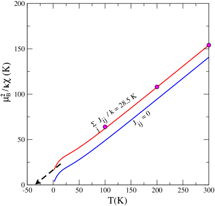
Figure 6: (Color online) Inverse susceptibility, $1/\chi$. The dots are data points taken from the more extensive data set of Ref. 35. The lower (online blue) curve is for $\lambda=0$ and the upper (online red) one is correct to first order in $\lambda$ [using Eq. (188)] for $\sum_{j}J_{ij}/k=28.5K$. For this curve the intercept extrapolated from $280{\rm K}<T<300{\rm}$ is $-33$K, as indicated by the arrow. The intercept extrapolated from infinite temperature is $\theta_{\rm C-W}=-(21/20)\sum_{j}J_{ij}=-30$K. So even at $T=300$K there is still a noticeable departure [of order $(T_{Q}/T)^{2}$] from the infinite temperature behavior.

Appendix C EFFECTIVE INTERACTIONS VIA EXCITED QUARTET STATES

Here we consider effective interactions which occur via excited virtual crystal field states. In a general formulation one considers manifolds ${\cal M}_{n}$ in which $n$ spins are in their excited quartet crystal field level, whose energy is $kT_{Q}$ relative to the crystal field ground state. We are interested in the effective Hamiltonian ${\cal H}_{0}$ for ${\cal M}_{0}$ at low temperature and here we discuss its evaluation within low order perturbation theory. We define

$${\cal H}_{n,m} = {\cal P}_{n}{\cal H}{\cal P}_{m}\ ,$$ (194)

where ${\cal P}_{n}$ is the projection operators for the manifold ${\cal M}_{n}$. Clearly the lowest approximation is to neglect entirely all processes except those within the manifold ${\cal M}_{0}$ and this was an implicit assumption of our calculations in the body of this paper. Processes involving virtual state in the manifold ${\cal M}_{1}$ enter via second order perturbation theory. These terms are obtained just as for superconductivity,CK with the result that

$${\cal H}_{0} = {\cal H}_{0,0}-{1\over kT_{Q}}\sum_{n}n^{-1}{\cal H}_{0,n}{\cal H}_{n,0}\ .$$ (195)

One can use this formalism to reproduce the formula for the zero-temperature Van Vleck susceptibility tensor,VV $\chi^{(V)}_{\alpha,\beta}$. However, our present aim is rather to analyze effective exchange interactions which arise in this way. To illustrate the phenomenon, consider contributions to Eq. (195) when ${\cal H}_{0,n}$ is taken to be the nn exchange interaction. Although we wrote this interaction as $K_{0}{\bf S}_{\rm eff,i}\cdot{\bf S}_{\rm eff,j}$ it really should be represented as $K^{\prime}{\bf J}_{i}\cdot{\bf J}_{j}$, where, since ${\bf S}_{\rm eff,i}=[(g_{J}-1)/g_{0}]{\bf J}_{i}=3/5{\bf J}_{i}$ one has that $K^{\prime}=(3/5)^{2}K_{0}=(9/25)K_{0}$. Then we obtain a contribution $V_{ij}$ to the effective nnn exchange interaction between spins $i$ and $j$ [at separation (a/2,a/2,0)] using the nn interactions $J_{ik}$ between spins $i$ and $k$ and $J_{kj}$ between $k$ and $j$. Since for a nnn pair $i,j$ there is only one choice for the intermediate site $k$ to be an nn of both sites $i$ and $j$, we have

$$V_{ij} = =-{{K^{\prime}}^{2}\over kT_{Q}}{\cal P}_{0}{\bf J}_{i}\cdot{\bf J}_{k}{\cal P}_{1}{\bf J}_{k}\cdot{\bf J}_{j}{\cal P}_{0}\ .$$ (196)

Because of the cubic symmetry of the crystal field one has

$${\cal P}_{0}J_{k,\alpha}{\cal P}_{1}J_{k,\beta}{\cal P}_{0}=(20/9)\delta_{\alpha,\beta}{\cal P}_{0}\ .$$ (197)

To obtain this result it is convenient to take $\alpha=\beta=z$ and use the ground state wavefunctions of Eq. (189). Then Eq. (196) yields

$$V_{ij} = -{20(9K_{0}/25)^{2}\over 9kT_{Q}}{\cal P}_{0}{\bf J}_{i}\cdot{\bf J}_{j}{\cal P}_{0}$$ (198)

$$= -{4K_{0}^{2}\over 5kT_{Q}}{\bf S}_{\rm eff,i}\cdot{\bf S}_{\rm eff,j}\ .$$

This means that due to these processes we have that

$$J\rightarrow J-{4K_{0}^{2}\over 5kT_{Q}}\equiv J-\delta J\ .$$ (199)

For $K_{0}/k=10$K and $T_{Q}=100$K, this gives $\delta J/k\approx 0.8$K. The nn interaction is renormalized in a similar way, except that if sites $i$ and $j$ are nn’s, then there are now two choices for the site $k$ to be an nn of both $i$ and $j$. Thus

$$K_{0}\rightarrow K_{0}-{8K_{0}^{2}\over 5kT_{Q}}\equiv K_{0}-\delta K_{0}\ ,$$ (200)

with $\delta K_{0}=1.6$K. As a final example, we similarly find for sites separated by $(a,0,0)$ that there are four intermediate paths of sites separated by $(a/2,a/2,0)$, so that

$$M\rightarrow M-{16J^{2}\over 5kT_{Q}}\equiv M-\delta M\ .$$ (201)

Taking $J/k=5$K, we find that $\delta M/k\approx 0.8$K, so that $\delta M/J=0.16$, a value which is comparable to those used in Table 2.

These results imply that even if the bare Hamiltonian only has nn interactions, virtual processes involving higher crystal field states will induce nnn interactions approximately of the size we will deduce from fitting experiments. This mechanism in higher order will produce significant longer range interactions even if the bare Hamiltonian has only nn interactions initially.

References

- (1) B. Barbara, J. X. Boucherle, J. L. Buevoz, M. F. Rossignol, and J. Schweizer, Solid State Commun. 24, 481 (1977).
- (2) B. Barbara, M. F. Rossignol, J. X. Boucherle, J. Schweizer, and J. L. Buevoz, J. Appl. Phys. 50, 2300 (1979).
- (3) S. M. Shapiro, E. Gurevitz, R. D. Parks, and L. C. Kupferberg, Phys. Rev. Lett. 34, 1748 (1979).
- (4) B. Barbara, M. F. Rossignol, J. X. Boucherle, and C. Vettier, Phys. Rev. Lett. 45, 938 (1980).
- (5) E. M. Forgan, B. D. Rainford, S. L. Lee, J. S. Abell, and Y. Bi, J. Phys. Condens. Matter 2, 10211 (1990).
- (6) F. Givord, J. Schweizer, and F. Tasset, Physica B 234-236, 685 (1997). The moment modulation quoted here should be corrected to read 23% rather than 15%.
- (7) K. H. J. Buschow and H. J. Van Daal, Phys. Rev. Lett. 23, 408 (1969).
- (8) B. Cornut and B. Coqblin, Phys Rev. B 5, 4541 (1972).
- (9) F. Ohkawa, Phys. Rev. B 66, 014408 (2002).
- (10) T. Nagamiya, in Solid State Physics, edited by F. Seitz and D. Turnbull (Academic, New York, 1967), Vol. 29, p 346.
- (11) R. M. Fleming, D. E. Moncton, D. B. McWhan, and F. J. DiSalvo, Phys. Rev. Lett. 45, 576 (1980).
- (12) S. Kawarazaki, K. Fujita, K. Yasuda, Y. Sasaki, T. Mizusaki, and A. Hirai, Phys. Rev. Lett. 61, 471 (1988).
- (13) T. Apih, U. Mikac, J. Seliger, J. Dolinsek, and R. Blinc, Phys. Rev. Lett. 80, 2225 (1998).
- (14) J. A. Paixao, C. Detlefs, M. J. Longfield, R. Caciuffo, P. Santini, N. Bernhoeft, J. Rebizant, and G. H. Lander, Phys. Rev. Lett. 89, 187202 (2002).
- (15) Y. Tokunaga, Y. Homma, S. Kambe, D. Aoki, H. Sakai, E. Yamamoto, A. Nakamura, Y. Shiokawa, R. E. Walstedt, and H. Yasuoka, Phys. Rev. Lett. 94, 137209 (2005).
- (16) D. Watson, E. M. Forgan, W. J. Nutall, W. G. Stirling, and D. Fort, Phys. Rev. B 53, 726 (1996).
- (17) K. A. McEwen and M. B. Walker, Phys. Rev. B 34, 1781 (1986). In this paper the stability of a double q state relative to a single q state was demonstrated.
- (18) Y. Yamamoto and T. Nagamiya, J. Phys. Soc. (Jpn) 32, 1248 (1971).
- (19) M. A. Ruderman and C. Kittel, Phys. Rev. 96, 99 (1954); T. Kasuya, Progr. Theoret. Phys. (Kyoto) 16, 45 (1956); K. Yosida, Phys. Rev. 106, 893 (1959).
- (20) A. B. Harris, C. Kallin, and A. J. Berlinsky, Phys. Rev. 45, 2899 (1992).
- (21) J. N. Reimers, A. J. Berlinsky, and A.-C. Shi, Phys. Rev. B 43, 865 (1991).
- (22) W. C. Koehler, R. M. Moon, and F. Holtzberg, J. Appl. Phys. 50, 1975 (1979).
- (23) Y. Lassailly, C. Vettier, F. Holtzberg, J. Floquet, C. M. E. Zeyen, and F. Lapierre, Phys. Rev. B 28, 2880 (1983).
- (24) Y. Nakanishi, T. Matsumura, F. Takahashi, T. Sakon, T. Suzuki, and M. Motokawa, J. Phys. Soc. Jpn. 70, 2703 (2001).
- (25) International Tables for Crystallography, (D. Riedel, Boston, 1993), Ed. T. Hahn, Vol. A.
- (26) N. W. Ashcroft and N. D. Mermin, Solid State Physics, (W. B. Saunders, Philadelphia, 1976).
- (27) R. W. Hill and J. M. Machado da Silva, Phys. Lett. 30A, 13 (1969).
- (28) C. Deenadas, A. W. Thompson, R. S. Craig, and W. E. Wallace, J. Phys. Chem Solids 32, 1853 (1971).
- (29) V. U. S. Rao and W. E. Wallace, Phys. Rev. B 2, 4613 (1971).
- (30) B. Barbara, J. X. Boucherle, J. P. Desclaux, M. F. Rossignol, and J. Schwiezer, in Crystal Field Effects in Metals and Alloys, Ed. A. Furrer (Plenum, New York, 1977), p 168.
- (31) For general spin the factor in Eq. (21) would be and would reproduce the correct for, say, a simple cubic ferromagnet.
- (32) In addition to systems in Refs. KAG, and PYR, wavevector selection fails for alkali-doped polyacetylene; see A. B. Harris, Phys. Rev. 50, 12441 (1994) and for the Kugel-Khomskii model; see A. B. Harris, A. Aharony, O. Entin-Wohlman, I. Ya. Korenblit, and T. Yildirim, Phys. Rev. B 69, 094409 (2004).
- (33) R. K. P. Zia and D. J. Wallace, J. Phys. A 8, 1495 (1975).
- (34) J. X. Boucherle and J. Schweizer, Physica 130B, 337 (1985).
- (35) W. M. Swift and W. E. Wallace, J. Phys. Chem. Solids 28, 2053 (1968).
- (36) E. Walker, H. G. Purwins, M. Landolt, and F. Hulliger, J. Less Common Metals 33, 203 (1973).
- (37) G. Lawes, M. Kenzelmann, N. Rogado, K. H. Kim, G. A. Jorge, R. J. Cava, A. Aharony, O. Entin-Wohlman, A. B. Harris, T. Yildirim, Q. A. Huang, S. Park, C. Broholm, and A. P. Ramirez, Phys. Rev. Lett. 93, 247201 (2004). M. Kenzelmann, A. B. Harris, A. Aharony, O. Entin-Wohlman, T. Yildirim, Q. Huang, S. Park, G. Lawes, C. Broholm, N. Rogado, R. J. Cava, K. H. Kim, G. Jorge, and A. P. Ramirez, to be published; cond-mat/0510386.
- (38) J. Schweizer, Comptes Rendus Physique 6, 375 (2005).
- (39) J. Schweizer, J. Villain, and A. B. Harris, to be published.
- (40) The minimum for occurs when only and are nonzero in which case assumes the value given by the right-hand side of Eq. (129). Then, if minimizes , so also does . Thus, at this level, the overall phase is not locked. The overall phase is locked by terms of th order in the ’s, such that the condition is very nearly satisfied.
- (41) L. D. Landau and E. M. Lifshitz, Statistical Mechanics (Addison-Wesley, New York, 1969).
- (42) For a full discussion see J. H. Van Vleck, Theory of Electric and Magnetic Susceptibilities, (Oxford U. P., Oxford, 1932). For a more modern application, see K. Gatterer and H. P. Fritzer, J. Phys. Condens. Matter 4, 4667 (1992).
- (43) C. Kittel, Quantum Theory of Solids, (Wiley, New York, 1963).