Angle-Resolved Photoemission Spectroscopy on Electronic Structure and Electron-Phonon Coupling in Cuprate Superconductors

I Introduction

In addition to the record high superconducting transition temperature (T_c), high temperature cuprate superconductorsBednorzMuller ; MKWuYBCO are characterized by their unusual superconducting properties below T_c, and anomalous normal state properties above T_c. In the superconducting state, although it has long been realized that superconductivity still involves Cooper pairsGough , as in the traditional BCS theorySchrieffer ; McMillan ; Marsiglio , the experimentally determined d$-$wave pairingTsuei is different from the usual s$-$wave pairing found in conventional superconductorsScalapino ; DPines . The identification of the pairing mechanism in cuprate superconductors remains an outstanding issueMagneticModePairing . The normal state properties, particularly in the underdoped region, have been found to be at odd with conventional metals which is usually described by Fermi liquid theory; instead, the normal state at optimal doping fits better with the marginal Fermi liquid phenomenologyMFLVarma . Most notable is the observation of the pseudogap state in the underdoped region above T_c Pseudogap . As in other strongly correlated electrons systems, these unusual properties stem from the interplay between electronic, magnetic, lattice and orbital degrees of freedom. Understanding the microscopic process involved in these materials and the interaction of electrons with other entities is essential to understand the mechanism of high temperature superconductivity.

Since the discovery of high-T_c superconductivity in cupratesBednorzMuller , angle-resolved photoemission spectroscopy (ARPES) has provided key experimental insights in revealing the electronic structure of high temperature superconductorsShenDessau ; DamascelliReview ; CampuzanoReview . These include, among others, the earliest identification of dispersion and a large Fermi surfaceOlsen , an anisotropic superconducting gap suggestive of a d$-$wave order parameterShenSCGap , and an observation of the pseudogap in underdoped samplesMarshall . In the mean time, this technique itself has experienced a dramatic improvement in its energy and momentum resolutions, leading to a series of new discoveries not thought possible only a decade ago. This revolution of the ARPES technique and its scientific impact result from dramatic advances in four essential components: instrumental resolution and efficiency, sample manipulation, high quality samples and well-matched scientific issues.

The purpose of this treatise is to go through the prominent results obtained from ARPES on cuprate superconductors. Because there have been a number of recent reviews on the electronic structures of high-T_c materialsShenDessau ; DamascelliReview ; CampuzanoReview , we will mainly present the latest results not covered previously, with a special attention given on the electron-phonon interaction in cuprate superconductors. What has emerged is rich information about the anomalous electron-phonon interaction well beyond the traditional views of the subject. It exhibits strong doping, momentum and phonon symmetry dependence, and shows complex interplay with the strong electron-electron interaction in these materials.

II Angle-Resolved Photoemission Spectroscopy

II.1 Principle

Angle-resolved photoemission spectroscopy is a powerful technique for studying the electronic structure of materials(Fig. 1)SHuefner . The information of interest, i.e., the energy and momentum of electrons in the material, can be inferred from that of the photoemitted electrons. This conversion is made possible through two conservation laws involved in the photoemission process:
(1). Energy conservation: E_B=h$\nu$-E_kin-$\Phi$;
(2). Momentum conservation: K_||=k_||+G.
where E_B represents the binding energy of electrons in the material; h$\nu$ the photon energy of incident light; E_kin the kinetic energy of photemitted electrons; $\Phi$ work function; k_|| momentum of electrons in the material parallel to sample surface; K_|| projected component of momentum of photoemitted electrons on the sample surface which can be calculated from the kinetic energy by $\hbar$K_||=$\sqrt{2mE_{kin}}$sin$\theta$ with $\hbar$ being Planck constant; G reciprocal lattice vector. Therefore, by measuring the intensity of the photoemitted electrons as a function of the kinetic energy at different emission angles, the electronic structure of the material under study, i.e., energy and momentum of electrons, can be probed directlySHuefner .

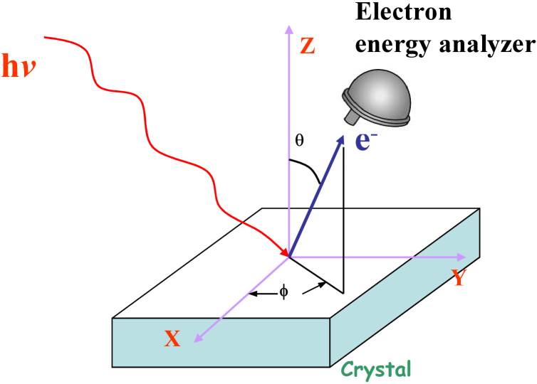
Figure 1: Schematic of angle-resolved photoemission spectroscopy.

For 3-dimensional materials, the electronic structure also relies on k_⊥, the momentum perpendicular to the sample surface. Because of the symmetry breaking near the sample surface, the momentum perpendicular to the sample surface is not conserved. In order to obtain k_⊥, one has to consider the inner potential which can be obtained in various waysSHuefner . For strictly 2-dimensional materials or quasi-2-dimensional materials such as the cuprate superconductors discussed in this treatise, to the first approximation, one may treat k_⊥ as a secondary effect. However, one should always be wary about the residual 3-dimensionality in these materials and its effect on photoemission dataBansilKzEffect .

The photoemission process can be understood intuitively in terms of a “three step model”Spicer : (i) Excitation of the electrons in the bulk by photons. (ii) Transport of the excited electrons to the surface. (iii) Emission of the photoelectrons into vacuum. Under the “sudden approximation” (described below), photoemission measures the single$-$particle spectral function A(k,$\omega$), weighted by the matrix element M and Fermi function f($\omega$): I$\sim$A(k,$\omega$)$\mid$M$\mid$²f($\omega$)Hedin ; Randeria . The matrix element $\mid$M$\mid$² term indicates that, besides the energy and momentum of the initial state and the final state, the measured photoemission intensity is closely related to some experimental details, such as energy and polarization of incident light, measurement geometry and instrumental resolution. The inclusion of the Fermi function accounts for the fact that the direct photoemission measures only the occupied electronic states.

The single-particle spectral function A(k,$\omega$) can be written in the following way using the Nambu-Gorkov formalism:

$$A(k,\omega)=-(1/\pi)ImG_{11}(k,\omega)$$ (1)

$$\widehat{G}(k,\omega)={\frac{Z(k,\omega)\omega\tau_{0}+(\varepsilon(k)+\chi(k,\omega))\tau_{2}+\phi(k,\omega)\tau_{1}}{{(Z(k,\omega)\omega)}^{2}-{(\varepsilon(k)+\chi(k,\omega))}^{2}-{\phi(k,\omega)}^{2}}}$$ (2)

where Z, $\chi$, and $\phi$ represent a renormalization due to either electron-electron or electron-phonon interactions and $\varepsilon(k)$ is the bare-band energy. $\tau_{0},\tau_{1},\tau_{2}$ are the matrices, and G₁₁ represents the Pauli electronic charge density channel measured in photoemission. In the weak coupling case, Z=1, $\chi=0$, and $\phi=\Delta$, the superconducting gap. The same formalism can be extended to the normal state by setting $\phi=0$. In the normal state, the spectral function can be written in a more compact wayHedin ; Randeria , in terms of the real and imaginary parts of the electron self energies Re$\Sigma$ and Im$\Sigma$:

$$A(k,\omega)=\frac{1}{\pi}\frac{|{\rm Im}\Sigma(k,\omega)|}{(\omega-\varepsilon(k)-{\rm Re}\Sigma(k,\omega))^{2}+({\rm Im}\Sigma(k,\omega))^{2}}$$ (3)

where Re$\Sigma$ describes the renormalization of the dispersion and Im$\Sigma$ describes the lifetime.

In relating the photoemission process in terms of single particle spectral function A(k,$\omega$), it is helpful to recognize some prominent assumptions involved:

(1). The excited state of the sample (created by the ejection of the photo-electron) does not relax in the time it takes for the photo-electron to reach the detector. This so-called “sudden-approximation” allows one to write the final state wave-function in a separable form, $\Psi_{f}^{N}=\Phi_{f}^{k}\Psi_{f}^{N-1}$, where $\Phi_{f}^{k}$ denotes the photoelectron and $\Psi_{f}^{N-1}$ denotes the final state of the material with N-1 electrons. If the system is non-interacting, then the final state overlaps with a single eigenstate of the Hamiltonian describing the N-1 electrons, revealing the band structure of the single electron. In the interacting case, the final state can overlap with all possible eigenstates of the N-1 system.
(2) In the interacting case, A($k,\omega$) describes a “quasiparticle” picture in which the interactions of the electrons with lattice motions as well as other electrons can be treated as a perturbation to the bare band dispersion, $\varepsilon(k)$, in the form of a self energy, $\Sigma(k,\omega)$. The validity of this picture as well as (1) rests on whether or not the spectra can be understood in terms of well-defined peaks representing poles in the spectral function.
(3). The surface is treated no differently from the bulk in this A($k,\omega$). In reality surface states are expected and are observed and can lead to confusion in the data interpretationDamascelliReview . Surface termination also affects photoemission processBansilMatrixBi2212 .

In addition to the matrix element M, there are other extrinsic effects which contribute to measured photoemission spectrum, e.g., the contribution from inelastic electron scattering. On the way to get out from inside the sample, the photoemitted electrons will experience scattering from other electrons, giving rise to a relatively smooth background in the photoemission spectrum.

II.2 Technique

As seen in Fig.1, an ARPES system consists of a light source, chamber and sample manipulation and characterization systems, and an electron energy analyzer. Fig.2 is an example of a modern ARPES setup with the following primary components:

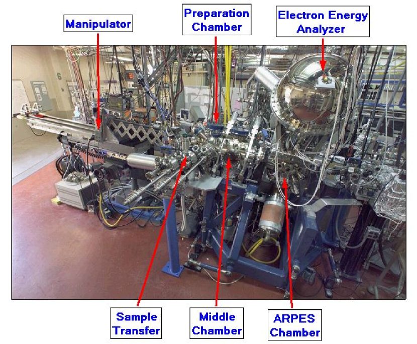
Figure 2: A representative ARPES system on Beamline 10.0.1 at the Advanced Light Source, Lawrence Berkeley National Lab.

(1). Light source: Possible light sources for angle-resolved photoemission are X-ray tubes, gas-discharge lamps, synchrotron radiation source and VUV lasers. Among them, the synchrotron radiation source is the most versatile in that it can provide photons with continuously tunable energy, fixed or variable photon polarization, high energy resolution and high photon flux. The latest development of the VUV laser is significant as a result of its super-high energy resolution and super-high photon flux. In addition, the lower photon energy achievable by the VUV lasers makes the measured electronic structure more bulk-sensitive in certain materialsTKissLaser . However, the strong final state effect may limit its application to certain material systems.

(2). Chambers and sample manipulation and characterization systems: In most of the photon energy range commonly used (20$\sim$100 eV), the escape depth of photoemitted electrons is on the order of 5$\sim$20 $\AA$, as seen in Fig.3SeahDench . This means that photoemission is a surface-sensitive technique. Therefore, obtaining and retaining a clean surface during measurement is essential to probe the intrinsic electronic properties of the sample. To achieve this, the ARPES measurement chamber has to be in ultra-high vacuum, typically better than 5$\times$10^-11 Torr. A clean surface is usually obtained either by cleaving samples in situ in the chamber if the samples are cleavable or by sputtering and annealing process if the sample is hard to cleave. The quality of the surface can be characterized by low energy electron diffraction (LEED) or other techniques such as scanning tunneling microscopy (STM). The sample transfer system is responsible for quickly transferring samples from air to UHV chambers while not damaging the ultra-high vacuum. The manipulator is responsible for controlling the sample position and orientation, it also holds a cryostat that can change the sample temperature during the measurement. An advanced low temperature cryostat which can control the sample temperature precisely and has multiple degrees of translation and rotation freedoms is critical to an ARPES measuremnet.

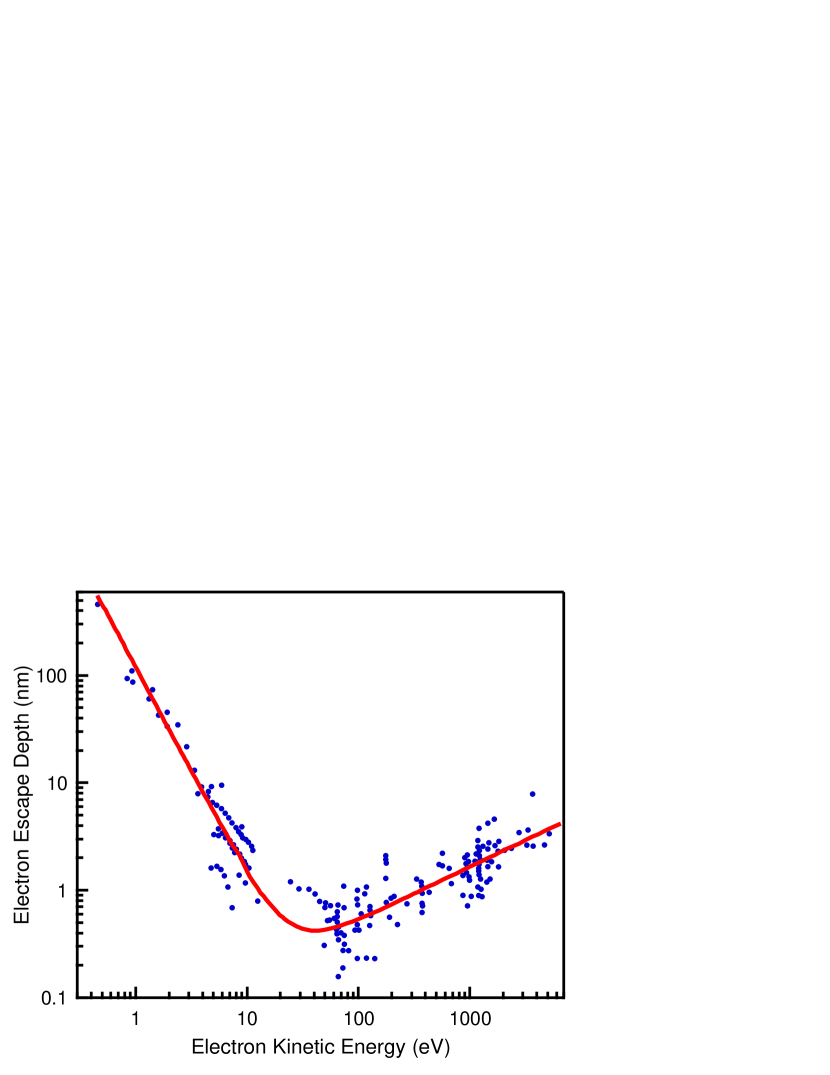
Figure 3: Escape depth of photoemitted electron as a function of kinetic energySeahDench . For elements and inorganic compounds, the escape depth is found to follow the ”universal curve” (red solid line).

(3). Electron energy analyzer: An analyzer measures the intensity of photoemitted electrons as a function of their kinetic energy, i.e., Energy Distribution Curve(EDC), at a given angle relative to the sample orientation. The dramatic improvement of the ARPES technique in the last decade is in large part due to the advent of modern electron energy analyzer, in particular, the Scienta series hemisphere analyzers. The enhancement of the performance lies in mainly three aspects:
(i). Energy resolution improvement.
The energy resolution of the electron energy analyzer improves steadily over time. The upgrade of the one-dimensional multichannel detection scheme of the VSW analyzer allows efficient measurement with $\sim$20meV energy resolution. Among others, it enabled the discovery of the d-wave superconducting gap structureShenSCGap . The first introduction of the Scienta 200 analyzer in the middle 1990’s dramatically improved the energy resolution to better than 5 meV. The latest Scienta R4000 analyzer has improved the energy resolution further to better than 1 meV, as seen in Fig.4TKissLaser .

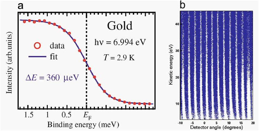
Figure 4: (a). Ultrahigh-resolution photoemission spectrum of an evaporated gold film measured using Scienta R4000 analyzer at a temperature of 2.9 K (red circles), together with the Fermi-Dirac function at 2.9 K convolved by a Gaussian with full width at half maximum of 360 $\mu$eV (a blue line). Total energy resolution of 360 $\mu$eV was confirmed from the very good match between the experimental and calculated spectraTKissLaser . The energy resolution from the VUV laser is estimated to be 260 $\mu$eV. (b). Angle mode testing image of Scienta R4000 electron analyzer. the test was performed using “wire-and-slit” setup, with the angle interval between adjacent slits being 1 degrees. In this particular angular mode, the analyzer collects emission angle within 30 degrees simultaneously.

We note that the total experimental energy resolution relies on both the analyzer resolution and the light source resolution. Sample temperature can also cause thermal broadening which is a limitation in some cases. The necessity of multiple degrees of rotation controls as well as the exposure of the surface during an ARPES measurement often puts a lower limit on the sample temperature. In addition, one should be aware of some intrinsic effects associated with the photoemission process, i.e., space charge effect and mirror charge effectZhouSCE . When pulsed light is incident on a sample, the photoemitted electrons experience energy redistribution after escaping from the surface because of the Coulomb interaction between them (space charge effect) and between photo-emitted electrons and the distribution of mirror charges in the sample (mirror charge effect). These combined Coulomb interaction effects give rise to an energy shift and a broadening whose magnitude depends on the photon energy, photon flux, beam spot size, emission angles and etc. For a typical third-generation synchrotron light source, the energy shift and broadening can be on the order of 10 meV (Fig.5)ZhouSCE . This value is comparable to many fundamental physical parameters actively studied by photoemission spectroscopy and should be taken seriously in interpreting photoemission data and in designing next generation experiments.

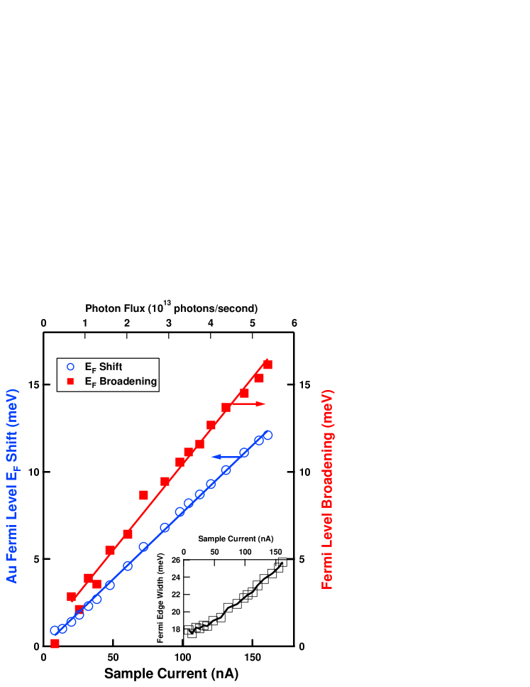
Figure 5: Space charge and mirror charge effect in photoemissionZhouSCE . Fermi edge broadening (solid square) and the Fermi edge shift (open circle) as a function of sample current. The beam spot size is $\sim$0.43mm$\times$0.30 mm. The inset shows the measured overall Fermi edge width as a function of the sample current, which includes all contributions including the beamline, the analyzer and the temperature broadening. The net broadening resulting from pulsed photons is obtained by deconvolution of the measured data, taking the width at low photon flux as from all the other contributions.

(ii). Momentum resolution;
The introduction of the angular mode operation in the new Scienta analyzers has also greatly improved the angular resolution, from a previous $\sim$2 degrees to 0.1$\sim$0.3 degree. This improvement of the momentum resolution allows one to observe detailed structures in the band structure and Fermi surface, as well as subtle but important many-body effects. As an example, recent identification of two Fermi surface sheets (so-called “bilayer splitting”)in Bi₂Sr₂CaCu₂O₈ (Bi2212) (Fig.6) is largely due to such an improvement of momentum resolutionFengBilayersplitting ; ChuangBilayerSplitting ; BogdanovBilayerSplitting , combined with the advancement of theoretical calculationsBansilMatrixBi2212 .

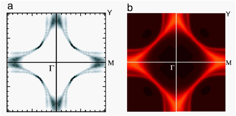
Figure 6: (a). Experimentally measured Fermi surface in Pb-doped Bi2212PashaBi2212 . (b). Calculated Fermi surface of Bi2212BansilMatrixBi2212 .

(iii). Two-dimensional multiple angle detection;
Traditionally, the electron energy analyzer collects one photoemission spectrum, i.e., energy distribution curve (EDC), at one measurement for each emission angle. Modern electron energy analyzers collect multiple angles simultaneously. As shown in Fig.4b, the latest Scienta R4000 analyzer can collect photoemitted electrons in the angle range of 30 degrees simultaneously. Therefore, at one measurement, the raw data thus obtained, shown in Fig.7a, is a 2-dimensional image of the photoelectron intensity (represented by false color) as a function electron kinetic energy and emission angle (and hence momentum). This 2-dimensionality greatly enhances data collection efficiency and provides a convenient way of analyzing the photoemission data.

As shown in Fig.7 , the traditional way to visualize the photoemission data is by means of so-called energy distribution curves (EDCs), which represent photoelectron intensity as a function of energy for a given momentum. The 2D image comprising the raw data is then equivalent to a number of EDCs at different momenta (Fig.7b). The peak position at different momenta will give the energy-momentum dispersion relation determining the real part of electron self-energy Re$\Sigma$. The EDC linewidth determines the quasiparticle lifetime, or the imaginary part of electron self-energy Im$\Sigma$. However, the EDC lineshape is usually complicated by a background at higher binding energy, the Fermi function cutoff near the Fermi level, and an undetermined bare band energy which make it difficult to extract the electron self-energy precisely.

An alternative way to visualize the 2D data is to analyze photoelectron intensity as a function of momentum for a given electron kinetic energyAebiMDC by means of momentum distribution curves (MDCs)VallaScience ; LashellBe . This approach provides a different way of extracting the electron self-energy. As shown in Fig.7c, the MDCs exhibit well-defined peaks with flat backgrounds; moreover, they can be fitted by a Lorentzian lineshape. When the bandwidth is large, the band dispersion $\epsilon$_k can be approximated as $\epsilon$_k = v₀k in the vicinity of the Fermi level. Under the condition that the electron self-energy shows weak momentum dependence, A(k,$\omega$) indeed exhibits a Lorentzian lineshape as a function of k for a given binding energy . By fitting a series of MDCs at different binding energies to obtain the MDC position $\tilde{k}$ and width $\Gamma$ (full-width at half maximum, FWHM) (Fig.7d)XJZhouJSR , one can extract the electron self-energy directly as: Re$\Sigma$=$\hbar$$\omega$-$\tilde{k}$v₀ and Im$\Sigma$=$\Gamma$v₀/2.

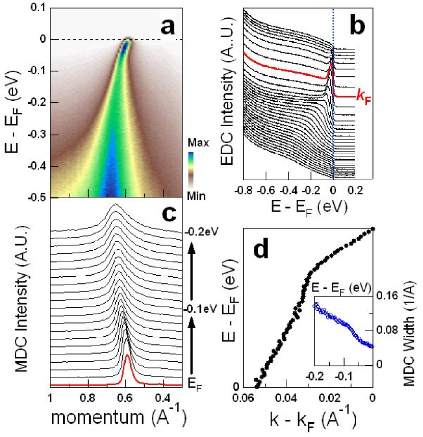
Figure 7: Illustration of the MDC method for extracting the electron self-energy. (a) Raw photoemission data for LSCO with x=0.063 (T_c$\sim$12K) along the (0,0)-($\pi$,$\pi$) nodal direction at 20 KXJZhouJSR . The two-dimensional data represent the photoelectron intensity (denoted by false color) as a function of energy and momentum. (b) Energy distribution curves (EDCs) at different momenta. The EDC colored red corresponds to the Fermi momentum k_F. (c) Momentum distribution curves (MDCs) at different binding energies. The MDC colored red corresponds to the Fermi level. (d) Energy-momentum dispersion relation extracted by the MDC method. The inset shows the MDC width as a function of energy.

It is worthwhile to point out the latest effort in attempting to overcome the surface sensitivity issue related with photoemission. As seen from Fig.3, in the usual photon energy range used for valence band photoemission, the photoemitted electron escape depth is on the order on 5$\sim$10 $\AA$. Therefore, it is always an issue whether the photoemission results obtained in this energy range represents the bulk properties. To overcome such a problem, there have been two approaches by employing either high photon energy or lower photon energy. As seen from Fig.3, when the photon energy is on the order of 1 KeV, the electron escape depth can be increased to $\sim$20 $\AA$SugahigheV . However, this modest enhancement of the bulk sensitivity comes at a price of sacrificing both the energy resolution and momentum resolution. On the other hand, when the photon energy is low, one can see that the electron escape depth increases dramatically. Note that this “universal” curve is obtained from metals, whether the same curve can be applied to oxide materials remains unclear yet. In addition to the potential engancement of the bulk sensitivity, one may further improve the energy and momentum resolution by going to lower photon energy..

III Electronic Structures of High Temperature Superconductors

III.1 Basic Crystal Structure and Electronic Structure

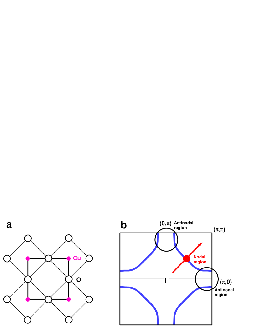
Figure 8: (a) Schematic of the real-space CuO₂ plane. The CuO₂ plane consists of copper (pink solid circles) and oxygen (black open circles). (b) The corresponding Brillouin zone in a reciprocal space. In the first Brillouin zone, the area near ($\pi$/2, $\pi$/2) (denoted as red circle) is referred to as nodal region, and the (0,0)-($\pi$,$\pi$) direction is the nodal direction (red arrow). The area near ($\pi$,0) and (0,$\pi$) is referred to as the antinodal region (shaded circles). The blue solid line shows a schematic Fermi surface.

A common structural feature of all cuprate superconductors is the CuO₂ plane (Fig.8a) which is responsible for the low lying electronic structure; the CuO₂ planes are sandwiched between various block layers which serve as charge reservoirs to dope CuO₂ planesTokura ; RJCava . For the undoped parent compound, such as La₂CuO₄, the valence of Cu is 2+, corresponding to 3d⁹ electronic configuration. Since the Cu²⁺ is surrounded by four oxygens in the CuO₂ plane and apical oxygen(s)or halogen(s) perpendicular to the plane, the crystal field splits the otherwise degenerate five d-orbitals, as schematically shown in Fig.9PickettRMP . The four lower energy orbitals, including xy, xz, yz and 3z² - r², are fully occupied, while the orbital with highest energy, x²-y², is half-filled. since the energies of the Cu d-orbitals and O 2p-orbitals are close, there is a strong hybridization between them. As a result, the topmost energy level has both Cu d${}_{x^{2}-y^{2}}$ and O 2p_x,y character.

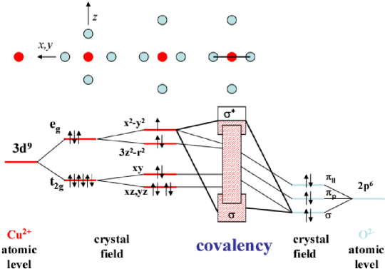
Figure 9: Bonding in CuO₂ planeFinkBond . The atomic Cu 3d level is split due to the cubic crystal field into e_g and t_2g states. There is a further splitting due to an octahedral crystal field into x² - y², 3z² - r², xy, and xz, yz states. For divalent Cu which has nine 3d electrons, the uppermost x² - y² level is half filled, while all other levels are completely filled. There is a strong hybridization of the Cu states, particularly the x² - y² states, with the O 2p states thus forming a half-filled two-dimensional Cu 3d${}_{x^{2}-y^{2}}$-O 2p_x,y antibonding dp$\sigma$ band. The hybridization of the other 3d levels is smaller and is indicated in Figure only by a broadening.

The same conclusion is also drawn from band structure calculations (Fig.10a)PickettRMP . According to both simple valence counting (Fig.9) and band structure calculation (Fig.10a), the undoped parent compound is supposed to be a metal. However, strong Coulomb interactions between electrons on the same Cu site makes it an antiferromagnetic insulator with an energy gap of 2 eVSUchidaGap ; VakninNeutron . The basic theoretical model for the electronic structure most relevant to our discussion is the multi-band Hubbard HamiltonianEmery ; VarmaModel containing d states on Cu sites, p states on O sites, hybridization between Cu-O states, hybridization between O-O states, and Coulomb repulsion terms. In terms of hole notation, i.e., starting from the filled-shell configuration (3d¹⁰,2p⁶) corresponding to a formal valence of Cu¹⁺ and O^2-, the general form of the model can be written asRiceLecture :

$$H=\sum_{i\sigma}\varepsilon_{d}d^{+}_{i\sigma}d_{i\sigma}+\sum_{l\sigma}\varepsilon_{p}p^{+}_{l\sigma}p_{l\sigma}+\sum_{<li>\sigma}t_{pd}p^{+}_{l\sigma}d_{i\sigma}+h.c.\\$$

$$+\sum_{i}U_{d}n_{i\uparrow}n_{i\downarrow}+\sum_{<ll^{\prime}>\sigma}t_{O-O}p^{+}_{l\sigma}p_{l^{\prime}\sigma}+h.c.$$

$$+\sum_{<il>\sigma\sigma^{\prime}}U_{pd}n_{l\sigma}n_{i\sigma^{\prime}}+\sum_{l}U_{p}n_{l\uparrow}n_{l\downarrow}$$ (4)

where the operator $d^{+}_{i\sigma}$ creates Cu (3d${}_{x^{2}-y^{2}}$)holes at site $i$, and $p^{+}_{l\sigma}$ creates O(2p) holes at the site $l$. U_d is the on-site Coulomb repulsion between two holes on a Cu site. The third term accounts for the direct overlap between Cu-O orbitals. The fifth terms describes direct hopping between nearest-neighbor oxygens, and U_pd in the sixth term is the nearest neighbor Coulomb repulsion between holes on Cu and O atoms. Qualitatively, this model gives the energy diagram in Fig.10c.

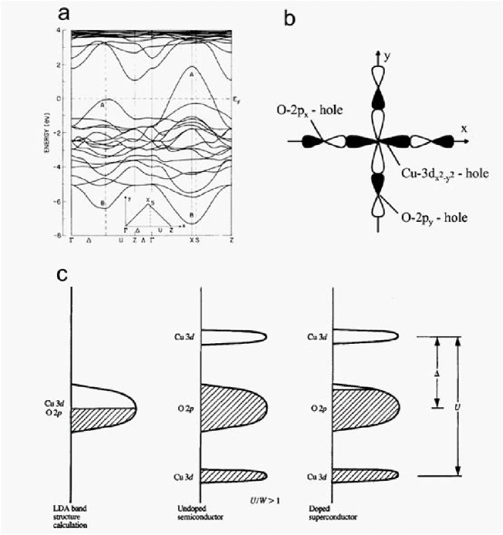
Figure 10: (a). LDA calculated band structure of La₂CuO₄MattheissLCO . The band labeled B is bonding band between Cu 3d${}_{x^{2}-y^{2}}$ and O 2p states while the band labeled A is the corresponding antibonding band that is half-filled; (b). Schematic of Zhang-Rice singlet stateZhangRice ; CDurr . (c). Schematic energy diagrams for undoped and doped CuO₂ planesSUchidaGap . (c1). Band picture for a half-filled (undoped) CuO₂ plane (Fermi liquid); (c2). Charge-transfer insulating state of the CuO₂ plane with split Cu 3d bands due to on-site Coulomb repulsive interaction $U$. The O 2p band is separated by a charge transfer energy $\Delta$ from the upper Cu 3d band; (c3) and (c4) show rigid charge transfer energy bands doped with holes and electrons, respectively; (c4). Formation of mid-gap states inside the charge transfer gap.

Simplified versions of model Hamiltonians have also been proposed. Notably among them are the single-band Hubbard modelAndersonRVB and t-J modelZhangRice . The t-J Hamiltonian can be written in the following formDagottoRMP ; RiceLecture :

$$H_{tJ}=-t\sum_{<ij>,\sigma}(\tilde{c}_{i\sigma}^{\dagger}\tilde{c}_{j\sigma}+H.c.)+J\sum_{<ij>}({\bf S_{i}}\cdot{\bf S_{j}}-\hat{n}_{i\uparrow}\hat{n}_{j\downarrow}/4)$$ (5)

where the operator $\tilde{c}_{i\sigma}^{\dagger}$=$c_{i\sigma}^{\dagger}(1-\hat{n}_{i-\sigma}$) excludes double occupancy, $J=4t^{2}/U$ is the antiferromagnetic exchange coupling constant, and S_i is the spin operator. Since the hopping process may also involve the second (t${}^{{}^{\prime}}$) and third (t^") nearest neighbor, an extended t-J model, the t$-$ t${}^{{}^{\prime}}$$-$t^"$-$J model, has also been proposedTTohyama .

III.2 Brief Summary of Some Latest ARPES Results

ARPES has provided key information on the electronic structure of high temperature superconductors, including the band structure, Fermi surface, superconducting gap, and pseudogap. These topics are well covered in recent reviewsDamascelliReview ; CampuzanoReview that we will not repeat here. Instead, we briefly summarize some of the latest developments not included before.

Band structure and Fermi surface: The bi-layer splitting of the Fermi surface is well established in the overdoped Bi2212FengBilayersplitting ; ChuangBilayerSplitting ; BogdanovBilayerSplitting , as shown in Fig.6 and also suggested to exist in underdoped and optimally doped Bi2212ChuangBS ; FengBS ; GromkoAntinodalKink ; KordyukBS . Recent measurements also show that there is a slight splitting along the (0,0)-($\pi$,$\pi$) nodal directionKordyukNodalBS . The measurement on four-layered Ba₂Ca₃Cu₄O₈F₂ has identified at least two clear Fermi surface sheetsYLChenBCCO .

Superconducting gap and pseudogap: Since the first identification of an anisotropic superconducting gap in Bi2212ShenSCGap , subsequent measurements on the superconductors such as Bi2212Bi2212SCGap1 ; Bi2212SCGap2 ; Bi2212SCGap3 ; Bi2212SCGap4 , Bi2201Bi2201SCGap1 ; Bi2201SCGap2 , Bi2223Bi2223SCGap1 ; Bi2223SCGap2 ; Bi2223SCGap3 , YBa₂Cu₃O_7-δYBCOSCGap , LSCOLSCOSCGap have established a universal behavior of the anisotropic superconducting gap in these hole-doped superconductors which is consistent with d-wave pairing symmetry (although it is still an open question whether the gap form is a simple d-wave-like $\Delta(k)$=$\Delta_{0}$[cos(k_xa)-cos(k_ya)] or higher harmonics of the expansion should be included). The measurements on electron-doped superconductors also reveal an anisotropic superconducting gapElectronSCGap1 ; ElectronSCGap2 .

One interesting issue is, if a material has multiple Fermi surface sheets, whether the superconducting gap on different Fermi surface sheets is the same. This issue traces back to superconducting SrTiO₃ where it was shown from tunneling measurements that different Fermi surface sheets may show different Fermi surface gapsBednorzSrTiO3 . With the dramatic advancement of the ARPES technique, different superconducting gaps on different Fermi surface sheets have been observed in 2H-NbSe₂TokoyaNbSe2 and MgB₂SoumaMgB2 . For high-T_c materials, Bi2212 shows two clear FS sheets, but no obvious difference of the superconducting gas has been resolvedBi2212SCGap4 . In Ba₂Ca₃Cu₄O₈F₂, it has been clearly observed that the two Fermi surface sheets have different superconducting gapsYLChenBCCO .

Time reversal symmetry breaking: It has been proposed theoretically that, by utilizing circularly polarized light for ARPES, it is possible to probe time-reversal symmetry breaking that may be associated with the pseudogap state in the underdoped samplesVarmaTRS ; SimonTRS . Kaminski et al. first reported the observation of such an effectKaminskiTRS . However, this observation is not reproduced by another groupBorisenkoTRS and the subject remain controversialTRSControversy .

IV Electron-Phonon Coupling in High Temperature Superconductors

The many-body effect refers to interactions of electrons with other entities, such as other electrons, or collective excitations like phonons, magnons, and so on. It has been recognized from the very beginning that many-body effects are key to understanding cuprate physics. Due to its proximity to the antiferromagnetic Mott insulating state, electron-electron interactions are extensively discussed in the literatureDamascelliReview ; CampuzanoReview . In this treatise, we will mostly review the recent progress in our understanding of electrons interacting with bosonic modes, such as phonons. This progress stems from improved sample quality, instrumental resolution, as well as theoretical development. In a complex system like the cuprates, it is not possible to isolate various degrees of freedom as the interactions mix them together. We will discuss the electron-boson interactions in this spirit, and will comment on the interplay between electron-phonon and electron-electron interactions whenever appropriate. Here by bosonic modes, we are referring to collective modes with sharp collective energy scale such as the optical phonons and the famous magnetic resonance mode seen in some cupratesResonanceModeYBCO ; ResonanceModeBi2212 ; RMHeTl2201 , but not the broad excitation spectra such as those from the broad electron/spin excitations as these issues have been discussed in previous reviews. Furthermore, we believe the effects due to sharp mode coupling seen in cuprates are caused by phonons rather than the magnetic resonance. Our reason for not attributing the observed effect to magnetic resonance will become apparent from the rest of the manuscript. With more limited data, other groups have taken the view that the magnetic resonance is the origin of the boson coupling effect. For this reason, we will focus more on our own results in reviewing the issues of electron-phonon interaction in cuprates.

The electron-phonon interactions can be characterized into two categories: (i). Weak coupling where one can still use the perturbative self-energy approach to describe the quasiparticle and its lifetime and mass; (ii). Strong coupling and polaron regime where this picture breaks down.

IV.1 Brief Survey of Electron-Phonon Coupling in High-Temperature Superconductors

It is well-known that, in conventional superconductors, electron-phonon (el-ph) coupling is responsible for the formation of Cooper pairsSchrieffer . The discovery of high temperature superconductivity in cuprates was actually inspired by possible strong electron-phonon interaction in oxides owing to polaron formation or in mixed-valence systemsBednorzMuller . However, shortly after the discovery, a number of experiments lead some people to believe that electron-phonon coupling may not be relevant to high temperature superconductivity. Among them arePBAllen :
(1). High critical transition temperature T_c
So far, the highest T_c achieved is 135 K in HgBa₂Ca₂Cu₃O₈SchillingNature at ambient pressure and $\sim$160 K under high pressureHgHighPressure . Such a high T_c was not expected in simple materials using the strongly coupled version of BCS theory, or the McMillan equations.
(2). Small isotope effect on T_c
It was found that the isotope effect in optimally-doped samples is rather small, much less than that expected for strongly-coupled phonon-mediated superconductivityBatloggIsotope .
(3). Transport measurement
The linear resistivity-temperature dependence in optimally doped samples and the lack of a saturation in resistivity over a wide temperature range have been taken as an evidence of weak electron-phonon coupling in the cuprate superconductorsGurvitchMartin .
(4).d-wave symmetry of the superconducting gap
It is generally believed that electron-phonon coupling is favorable to s-wave coupling.
(5). Structural instability.
It is generally believed that sufficiently strong electron-phonon coupling to yield high T_c will result in structural instabilityCohenAndersonTcLimit .

Although none of these observations can decisively rule out the electron-phonon coupling mechanism in high-T_c superconductors, overall they suggest looking elsewhere. Instead, strong electron-electron correlation has been proposed to be the mechanism of high-T_c superconductivity PAndersonBook . This approach is attractive since d$-$wave pairing is a natural consequence. Furthermore, the high temperature superconductors evolve from antiferromagnetic insulating compounds where the electron-electron interactions are strong Scalapino ; DPines

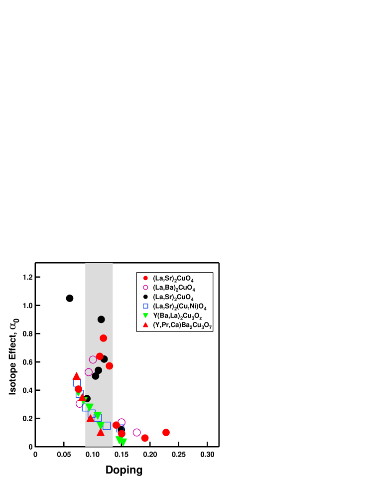
Figure 11: Doping dependence of the oxygen isotope effect $\alpha$₀ on T_c in several classes of cupratesIsoGMZhao ; CrawfordScience ; TSchneider . The ”1/8 anomaly” data found in LSCO system is highlighted in the shaded region.

However, there is a large body of experimental evidence also showing strong electron-phonon coupling in high-temperature superconductorsKAMuller ; Kulic ; MottAlexandrov . Among them are:

(1). Isotope effect;
As seen in Fig.11, although at the optimal doping, the oxygen isotope effect on T_c is indeed small, it gets larger and becomes significant with reduced dopingTSchneider . In particular, near the “1/8” doping level, the isotope effect in (La_2-xSr_x)CuO₄ and (La_2-xBa_x)CuO₄ is anomalously strong, which is related to the structural instabilityCrawfordScience . Furthermore, the measurement of an oxygen isotope effect on the in-plane penetration depth also suggests the importance of lattice vibration for high-T_c superconductivtyJHofer .

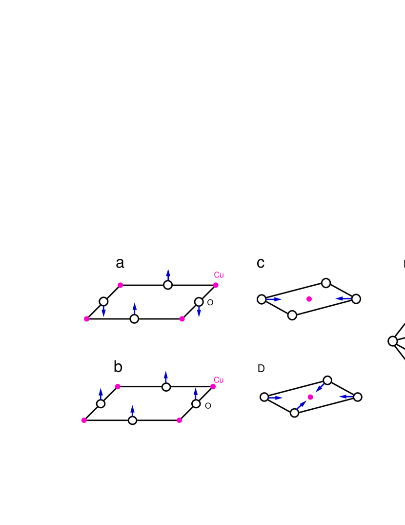
Figure 12: Schematic of B_1g mode (a), A_1g mode (b), half-breathing mode (c), full-breathing mode (d) and apical oxygen mode (e).

(2).Optical spectroscopy and Raman scattering;
Raman scatteringMCardonaPhonon and infrared spectroscopyTajimaIR reveal strong electron-phonon interaction for certain phonon modes. Some typical vibrations related to the in-plane and apical oxygens are depicted in Fig.12. In YBa₂Cu₃O_7-δ, it has been found that, the B_1g phonon, which is related to the out-of-plane, out-of-phase, in-plane oxygen vibrations (see Fig.12), exhibits a Fano-like lineshape (Fig.13) and shows an abrupt softening upon entering the superconducting stateCThomson_B1g ; Friedl ; AltendorfB1g . The A_1g modes, as found in HgBa₂Ca₃Cu₄O₁₀ (Hg1234)ZhouRaman and in HgBa₂Ca₂Cu₃O₈ (Hg1223)ZhouRaman1223 , exhibit especially strong superconductivity-induced phonon softening(Fig.14). Infrared reflectance measurements on various cuprates found that the frequency of the Cu-O stretching mode in the CuO₂ plane is very sensitive to the distance between copper and oxygenTajimaIR .

Fig. 15 shows Raman data as a function of doping in LSCOSugaiLSCO . The sharp structures at high frequency are signals from multiphonon processes, which can only occur if the electron-phonon interaction is very strong. One can see that this effect is very strong in undoped and deeply underdoped regime, and gets weaker with doping increase.

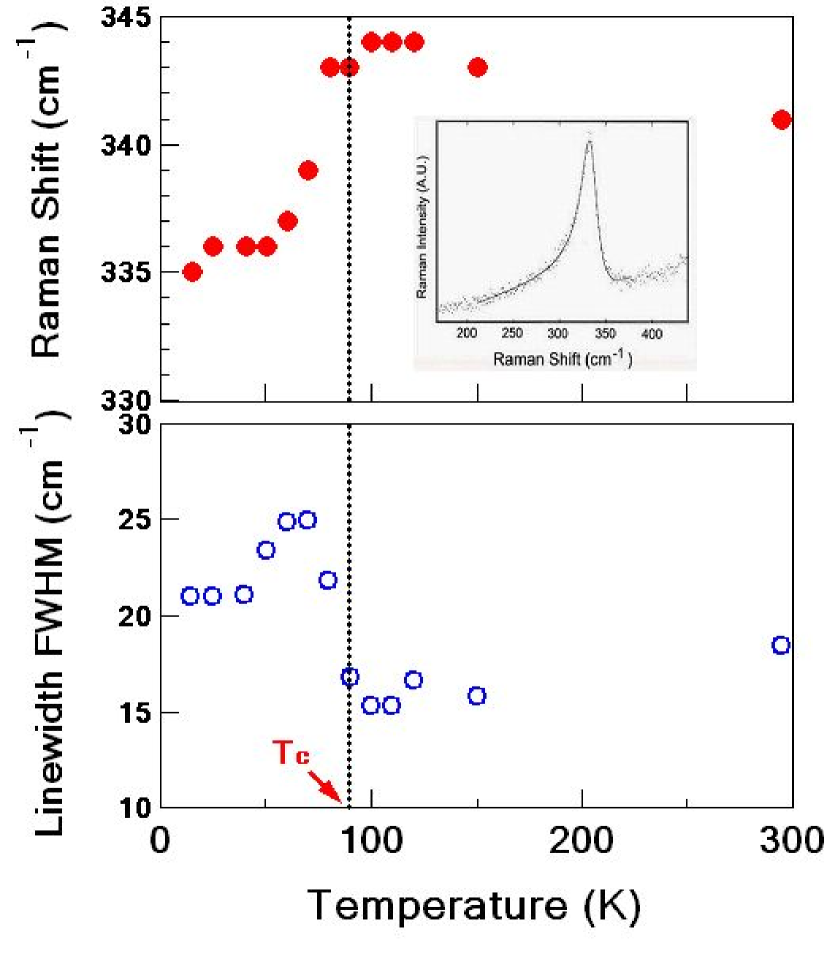
Figure 13: Anomalous softening of the B_1g phonon when YBCO is cooled below T_cAltendorfB1g . The inset shows the fit of a Fano function to the phonon peak at T=72KCThomson_B1g

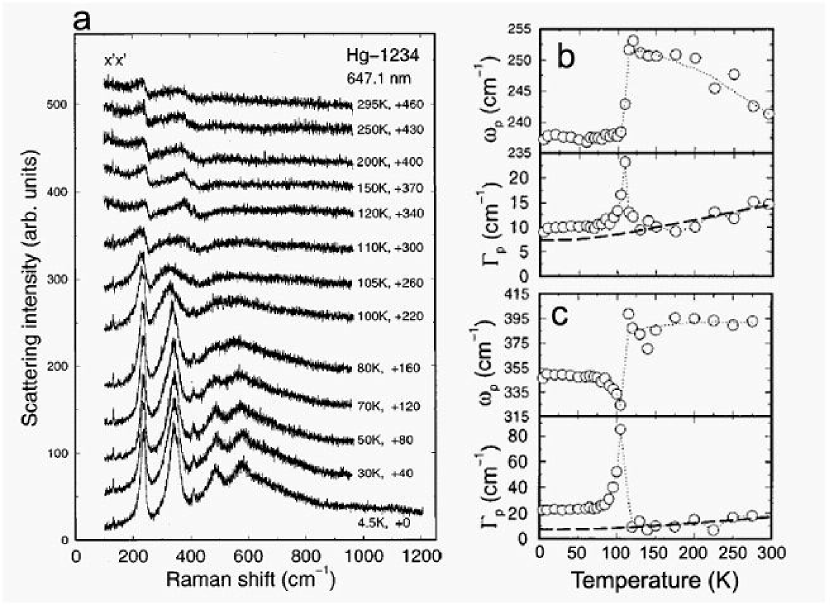
Figure 14: Raman spectra of Hg1234 showing a giant superconductivity-induced mode softening across T_c=123 KZhouRaman . The modes at 240 cm^-1 and 390 cm^-1 correspond to A_1g out-of-plane, in-phase vibration of oxygens in the CuO₂ planes. Upon cooling from room temperature to 4.5 K, the 240 cm^-1 A_1g mode shows a abrupt drop in frequency at T_c from 253 to 237 cm^-1 and the 390 cm^-1 mode drops from 395 to 317 cm^-1ZhouRaman .

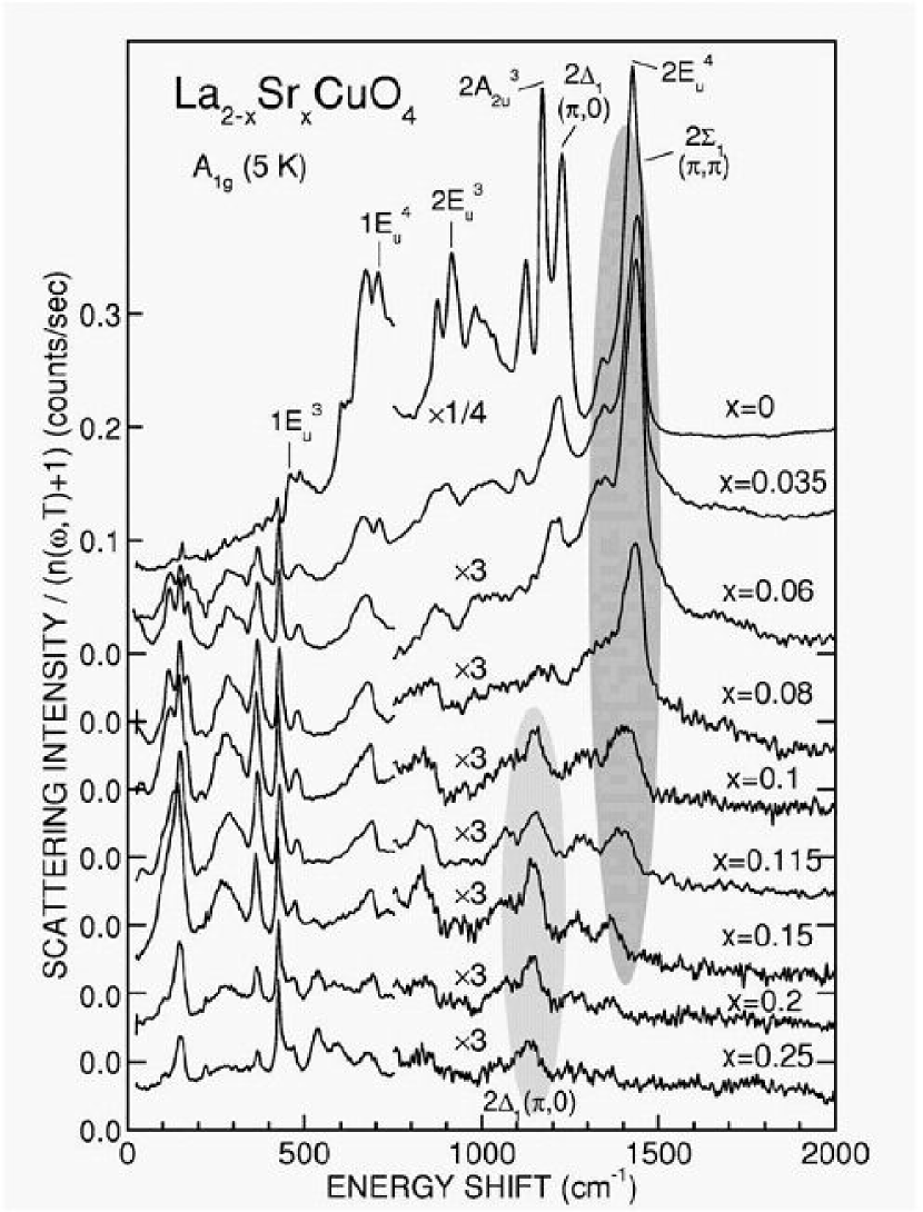
Figure 15: A_1g two-phonon Raman spectra in LSCO at different dopings. The dark gray area indicates that the two-phonon peak of the ($\pi$,$\pi$) LO mode is strong and the light gray area indicates that the two-phonon peak of the ( $\pi$,0) LO mode is strongSugaiLSCO .

(3). Neutron scattering
Neutron scattering measurements have provided rich information about electron-phonon coupling in high temperature superconductorsPintschoviusReview ; EgamiReview ; YBCOB1gNeutron . As seen from Fig.16a, the in-plane “half-breathing” mode exhibits strong frequency renormalizations upon doping along (001) directionPintschoviusBreathingMode ; PintschoviusReview . In (La_1.85Sr_0.15)CuO₄, it is reported that, at low temperature, the half-breathing mode shows a discontinuity in dispersion (Fig.16b)McQueeneyBreathingMode . In YBCO, neutron scattering indicates that the softening of the B_1g mode upon entering the superconducting state is not just restricted near q=0, as indicated by Raman scattering (Fig.13), but can be observed in a large part of the Brillouin zone (Fig.17)YBCOB1gNeutron .

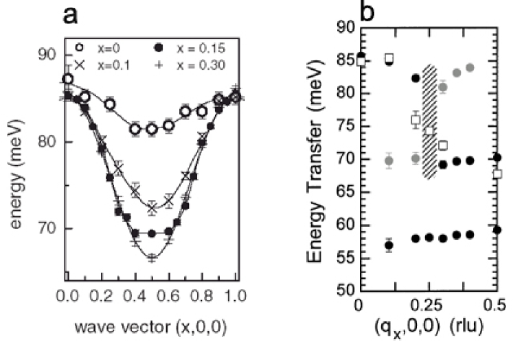
Figure 16: (a). Dispersion of the Cu-O bond-stretching vibrations in the (100)-direction in (La_2-xSr_x)CuO₄PintschoviusReview . (b). Anomalous dispersion of LO phonons in La_1.85Sr_0.15CuO₄. 10K data are filled circles and room temperature data are empty squares. Grey shaded circles indicate the frequency of the weak extra branch seen at 10KMcQueeneyBreathingMode .

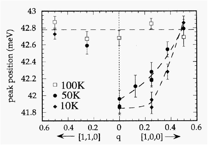
Figure 17: q dependence of B_1g mode peak position at different temperatures in YBCO. Dashed lines are guides to the eyeYBCOB1gNeutron

(4). Material and structural dependence;
There is a strong material and structural dependence to the high-T_c superconductivity, as exemplified in Fig.18)MaterialTc ; ShenPM . Empirically it is found that, for a given homologous series of materials, the optimal T_c varies with the number of adjacent CuO₂ planes, n, in a unit cell: T_c goes up first with n, reaching a maximum at n=3, and goes down as n further increases. For the cuprates with the same number of CuO₂ layers, T_c also varies significantly among different classes. For example, the optimal T_c for one-layered (La_2-xSr_x)CuO₄ is 40K while it is 95K for one-layered HgBa₂CuO₄. These behaviors are clearly beyond simplified models that consider CuO₂ planes only, such as the t$-$J model. In fact, such effects were taken as evidence against theoretical models based on such simple models and in favor of the interlayer tunneling modelAndersonILT . Although the interlayer tunneling model has inconsistencies with some experiments, the issue that the material dependence cannot be explained by single band Hubbard and t-J model remains to be true.

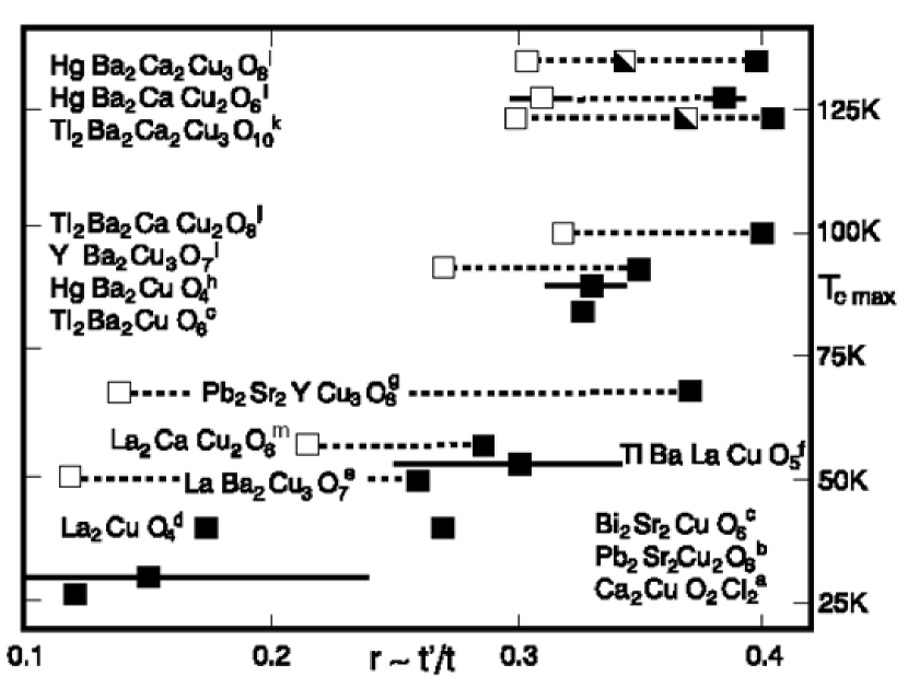
Figure 18: Correlation between calculated range parameter r and observed T_cmax where r is controlled by the energy of the axial orbital, a hybrid between Cu 4s, apical-oxygen 2p_z , and farther orbitalsMaterialTc . Filled squares: single-layer materials and most bonding subband for multilayers. Empty squares: most antibonding subband. Half-filled squares: nonbonding subband. Dotted lines connect subband values. Bars give k_z dispersion of r in primitive tetragonal materials, For reference for a-m, refer to MaterialTc .

The above results suggest that the lattice degree of freedom plays an essential role. However, the role of phonons has not been scrutinized as much, in particular in regard to the intriguing question of whether high-T_c superconductivity involves a special type of electron-phonon coupling. In other words, the complexity of electron-phonon interaction has not been as carefully examined as some of the electronic models. As a result, many naive arguments are used to argue against electron-phonon coupling as if the conclusions based on simple metals are applicable here. Recently, a large body of experimental results from angle-resolved photoemission, as we review below, suggest that electron-phonon coupling in cuprates is not only strong but shows behaviors distinct from conventional electron-phonon coupling. In particular, the momemtum dependence and the interaction between electron-phonon interaction and electron-electron interaction are very important.

IV.2 Electron-Phonon Coupling: Theory

IV.2.1 General

Theory of electron-phonon interaction in the presence of strong electron correlation has not been developed. Given both interactions are important in cuprates, it is difficult a priori to have a good way to address these issues. In fact, we believe that an important outcome of our research is the stimulus to develop such a theory. In the mean time, our strategy to separate the problem in different regimes and see to what extent we can develop a heuristic understanding of the experimental data. Such empirical findings can serve as a guide for comprehensive theory. We now start our discussion with an overview of existing theories of electron-phonon physics.

The theories of electron-phonon coupling in condensed matter have been developed rather separately for metals and insulators. In the former case, the dominant energy scale is the kinetic energy or the Fermi energy $\varepsilon_{F}$ on order of $1-10$eV, and the phonon frequency $\Omega\sim 1-100$meV is much smaller. The Fermi degeneracy protects the many-body fermion system from perturbations and only the small energy window near the Fermi surface responds. Therefore even if the lattice relaxation energy $E_{LR}=g^{2}/\omega$ for the localized electron is comparable to the kinetic energy $\varepsilon_{F}$ the el-ph coupling is essentially weak and the perturbative treatment is justified. The dimensionless coupling constant $\lambda$ is basically the ratio of $E_{LR}/\varepsilon_{F}$, which ranges $\lambda\cong 0.1-2$ in the usual metals. In the diagrammatic language, the physics described above is formulated within the framework of the Fermi liquid theoryAGD . The el-el interaction is taken care of by the formation of the quasi-particle, which is well-defined near the Fermi surface, and the el-ph vertex correction is shown to be smaller by the factor of $\Omega/\varepsilon_{F}$ and can be neglected. Therefore the multi-phonon excitations are reduced and the single-loop approximation or at most the self-consistent Born approximation is enough to capture the physics well, i.e., Migdal-Eliashberg formalism.

When a carrier is put into an insulator, on the other hand, it stays near the bottom of the quadratic dispersion and its velocity is very small. The kinetic energy is much smaller than the phonon energy, and the carrier can be dressed by a thick phonon cloud and its effective mass can be very large. This is called the phonon polaron. Historically the single carrier problem coupled to the optical phonon through the long range Coulomb interaction, i.e., Fröhlich polaron, is the first studied model, which is defined in the continuum. When one considers the tight-binding models, which is more relevant to the Bloch electron, the bandwidth $W$ plays the role of $\varepsilon_{F}$ in the above metallic case. Then again we have three energy scales, $W$, $E_{RL}$, and $\Omega$. Compared with the metallic case, the dominance of the kinetic energy is not trivial, and the competition between the itinerancy and the localization is the key issue in the polaron problem, which is controlled by the dimensionless coupling constant $\lambda=E_{RL}/W$. Another dimensionless coupling constant is $S=E_{RL}/\Omega$, which counts the number of phonon quanta in the phonon cloud around the localized electron. This appears in the overlap integral of the two phonon wavefunctions with and without the phonon cloud as:

$$<{\rm phonon\ \ vacuum}|{\rm phonon\ \ cloud}>\propto e^{-S}$$ (6)

This factor appears in the weight of the zero-phonon line of the spectral function of the localized electron, and $S$ can be regarded as the maximum value for the number of phonons $N_{\rm ph}$ near the electron. In a generic situation, $N_{\rm ph}$ is controlled by $\lambda$, and there are cases where $N_{\rm ph}$ shows an (almost) discontinuous change from the itinerant undressed large polaron to the heavily dressed small polaron as $\lambda$ increases. This is called the self-trapping transition. Here a remark on the terminology “self-trapping” is in order. Even for the heavy mass polaron, the ground state is the extended Bloch state over the whole sample and there is no localization. However a small amount of disorder can cause the localization. Therefore in the usual situation, the formation of the small polaron implies the self-trapping, and we use this language to represent the formation of the thick phonon clouds and huge mass enhancement. In cuprates, it is still a mystery why the transport properties of the heavily underdoped samples do not show the strong localization behavior even though the ARPES shows the small polaron formation as will be discussed in D.1.

Now the most serious question is what is the picture for the el-ph coupling in cuprates ? The answer seems not so simple, and depends both on the hole doping concentration, momentum and energy. The half-filled undoped cuprate is a Mott insulator with antiferromagnetic ordering, and a single hole doped into it can be regarded as the polaron subjected to the hole-magnon and hole-phonon interactions. At finite doping, but still in the antiferromagnetic (AF) order, the small hole pockets are formed and the hole kinetic energy can be still smaller than the phonon energy. In this case the polaron picture still persists. The main issue is to what range this continues. One scenario is that once the antiferromagnetic order disappears the metallic Fermi surface is formed and the system enters the Migdal-Eliashberg regime. However, there are several physical quantities such as the resistivity, Hall constant, optical conductivity, which strongly suggest that the physics still bears a strong characteristics of doped holes in an insulator rather than a simple metal with large Fermi surface. Therefore the crossover hole concentration $x_{c}$ between the polaron picture and the Migdal-Eliashberg picture remains an open issue. Probably, it depends on the momentum/energy of the spectrum. For example, the electrons have smaller velocity and are more strongly coupled to the phonons in the anti-nodal region near $(\pm\pi,0)$, $(0,\pm\pi)$, remaining polaronic up to higher doping, while in the nodal region, the electrons behave more like the conventional metallic ones since the velocity is large along this direction. Furthermore, the low energy states near the Fermi energy are well described by Landau’s quasi-particle and Migdal-Eliashberg theory, while the higher energy states do not change much with doping even at $x\cong 0.1$ KShenPolaron suggestive of polaronic behavior. In any event, the dichotomy between the hole doping picture and the metallic (large) Fermi surface picture is the key issue in the research of high T_c superconductors.

IV.2.2 Weak Coupling – Perturbative and Self-Energy Description

We review first the Migdal-Eliashberg regime, in which the electron-phonon interaction results in single-phonon excitations and can be considered as a perturbation to the bare band dispersion. In this case, dominant features of the mode coupling behavior can be captured using the following form for the self-energy:

$$\widehat{\Sigma}(k,\omega)=T/N\sum_{q,\nu}g^{2}(k,q)D(q,i\nu)\tau_{3}\widehat{G}(k-q,i\omega-i\nu)\tau_{3}$$ (7)

where $D(q,\omega)={\frac{2\Omega_{q}}{\omega^{2}-\Omega_{q}^{2}}}$ is the phonon propagator, $\Omega_{q}$ is the phonon energy, T is temperature, N is the number of particles and $\tau_{3}$ is the Pauli matrix.

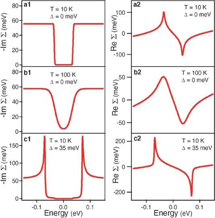
Figure 19: Self-energy for electrons coupled to an Einstein mode with $\Omega$ = 35 meV and electron-phonon vertex $g=0.15$ eVTanjaReview . (a1), (b1), and (c1) plots Im$\Sigma$= -$Z_{2}\omega+\chi_{2}$ for a normal state electron at 10 K, for a normal state electron at 100 K, and for an electron in an s-wave superconducting state at 10 K, respectively. (a2), (b2), and (c2) plots the corresponding real parts, Re$\Sigma$ , obtained using the Kramers-Kronig relation.

In this form of the self-energy, corrections to the electron-phonon vertex, $g$, are neglected as mentioned aboveMigdal . Furthermore, we assume only one-iteration of the coupled self-energy and Green’s function equations. In other words, in the equation for the self- energy, $\Sigma$, we assume bare electron and phonon propagators, G₀ and D₀. With these assumptions, the imaginary parts of the functions $Z$, $\chi$, and $\phi$, denoted as $Z_{2}$, $\chi_{2}$, and $\phi_{2}$, are:

$$Z_{2}(k,\omega)\omega=\sum_{q}g^{2}(k,q)(\pi/2)\{[\delta(\omega-\Omega_{q}-E_{k-q})$$

$$+\delta(\omega-\Omega_{q}+E_{k-q})][f(\Omega_{q}-\omega)+n(\Omega_{q})]$$

$$+[-\delta(\omega+\Omega_{q}-E_{k-q})-\delta(\omega+\Omega_{q}+E_{k-q})][f(\Omega_{q}+\omega)+n(\Omega_{q})]\}$$ (8)

$$\chi_{2}(k,\omega)=\sum_{q}g^{2}(k,q)(\pi\varepsilon_{k-q}/2E_{k-q})\{[-\delta(\omega-\Omega_{q}-E_{k-q})$$

$$+\delta(\omega-\Omega_{q}+E_{k-q})][f(\Omega_{q}-\omega)+n(\Omega_{q})]$$

$$+[\delta(\omega+\Omega_{q}-E_{k-q})-\delta(\omega+\Omega_{q}+E_{k-q})][f(\Omega_{q}+\omega)+n(\Omega_{q})]\}$$ (9)

$$\phi_{2}(k,\omega)=\sum_{q}g^{2}(k,q)(\pi\Delta_{k-q}/2E_{k-q})\{[\delta(\omega-\Omega_{q}-E_{k-q})$$

$$-\delta(\omega-\Omega_{q}+E_{k-q})][f(\Omega_{q}-\omega)+n(\Omega_{q})]$$

$$+[-\delta(\omega+\Omega_{q}-E_{k-q})+\delta(\omega+\Omega_{q}+E_{k-q})][f(\Omega_{q}+\omega)+n(\Omega_{q}]\}$$ (10)

where $f(x)$, $n(x)$, are the Fermi, Bose distribution functions and $E_{k}$ is the superconducting state dispersion, $E_{k}^{2}=\varepsilon_{k}^{2}+\Delta_{k}^{2}$.

The above equations are essentially those of Eliashberg theory for strongly-coupled superconductors. Although $\lambda$ can be large ($>1$), i.e., “strongly-coupled”, the vertex corrections and multi-phonon processes are still negligible due to the Fermi degeneracy and small $\Omega/E_{F}$Eliashberg . To illustrate the essential features of mode coupling, we consider an Einstein phonon coupled isotropically to a parabolic band. We present this calculation in the spirit of Engelsberg and Schrieffer, who first calculated the spectral function for an electron-phonon coupled systemEnglesberg and which provided the foundation for the later work by Scalapino, Schrieffer, and WilkinsPbTheory in the superconducting state. Fig.19 plots $-Z_{2}\omega+\chi_{2}$, the imaginary part of the phonon self-energy, Im$\Sigma$, that represents the renormalization to the diagonal channel of the electron propagator, or the one in which the charge number density is subjected to electron-phonon interactions. This part of the self-energy gives a finite lifetime to the electron, and consequently broadens the peak in the spectra (Im$\Sigma$ in $A(k,\omega)$ (Eq. 3) is the half-width-at-half-maximum, HWHM of the peak). In the normal state, $-Z_{2}\omega+\chi_{2}$ takes the familiar form:

$${\rm Im}\Sigma(k,\omega)=\Sigma_{q}-\pi g^{2}(k,q)[2n(\Omega_{q})+$$

$$f(\Omega_{q}+\omega)+f(\Omega_{q}-\omega)]\delta(\omega-E_{k-q})$$ (11)

which when integrated over q becomes:

$${\rm Im}\Sigma(k,\omega)=\int d\Omega\alpha^{2}_{k}F(\Omega)[2n(\Omega)+f(\Omega+\omega)+f(\Omega-\omega)]$$ (12)

where $\alpha^{2}_{k}F(\Omega)$, the Eliashberg function, represents the coupling of the electron with Fermi surface momentum $k$, to all $\Omega$ phonons connecting that electron to other points on the Fermi surface.

For the normal state electron at 10K (Fig.19a1), there is a sharp onset of the self-energy that broadens the spectra beyond the mode energy; for the normal state electron at 100K (Fig. 19b1), the onset of the self-energy is much smoother and occurs over $\sim$ 50meV; for the superconducting state electron (Fig. 19c1), there is a singularity that causes a much more abrupt broadening of the spectra at the energy $\Omega$ + $\Delta$. The superconducting state singularity is due to the density of states pile-up at the gap energy; the energy at which the decay onsets shift by $\Delta$, since below the gap energy there are no states to which a hole created by photoemission can decay. For each of these imaginary parts of the self-energy, one can use the Kramers-Kronig transform to obtain the real part of the self energy, which renormalizes the peak position (${\rm Re}\Sigma$ in $A(k,\omega)$ (Eq. 3) changes the position of the peak in the spectral function). The real self energies thereby obtained are also plotted in Fig. 19a2, Fig. 19b2, and Fig. 19c2. In the superconducting state, again there is a singularity that causes a more abrupt break from the bare-band dispersion at the energy $\Omega$ + $\Delta$.

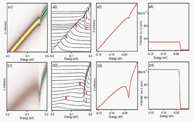
Figure 20: Simulated electron-phonon coupling using Einstein model. Spectral function (a1, b1), EDCs (a2, b2), MDC-derived dispersion (a3, b3), and the MDC-derived width (a4, b4) (imaginary part of self-energy) for two different couplings (a weak, b five times stronger) to a linear bare band.

For most metals, where the electrons are weakly interacting, and therefore the poles of the spectral function are well-defined, one would expect such a treatment to hold and indeed it does, as evidenced by several cases including BerylliumJensen ; Hensberger and MolybdenumVallaMo . A priori, one might not expect the same to hold in ceramic materials such as the copper-oxides, where the copper d-wave electrons are localized and subject to strong electron-electron and electron-phonon interactions. Nonetheless, in the superconducting state of the copper-oxides at optimal and overdoped regime, one recovers narrow peaks (20$\sim$30meV) of the spectral function. The above self-energy, then, is able to describe the phenomenology of the mode-coupling behavior for the superconducting state. The difference between the self-energy induced for a particular mode and coupling constant in the normal state at T=100K (Fig.19) and the superconducting state at T=10K (Fig.19) also shows the extent to which one can expect a temperature-dependent mode coupling in the high-T_c cuprates.

To illustrate the salient features of mode-coupling on the dispersion, we consider a linear bare band coupled to an Einstein phonon in the normal state at T=10K. The effect of electron-phonon interaction on the one-electron spectral weight $A(k,\omega)$ of a d${}_{x^{2}-y^{2}}$ superconductor has been simulated by Sandvik et al.Sandvik . In Fig.20, we show image plots, EDCs, MDC derived dispersions, and the MDC extracted widths for two different coupling constants (the case of stronger coupling is a factor of five increase in the vertex, $g^{2}$).

There are three characteristic signatures of mode coupling behavior evident:

1) A break up of a single dispersing peak into two branches(Fig.20a1 and b1)—a peak that decays as it asymptotically approaches the mode energy (I in Fig. 20a2 and b2), and a hump that traces out a dispersing band (II in Fig.20a2 and b2).

2) In the image plots (Fig.20a1 and b1), a significant broadening of the spectra beyond the mode energy is readily apparent. This is also the origin of the broad hump of the dispersing band seen in the EDCs (Fig.20a2 and b2) and the step in the extracted widths (or lifetime) (Fig.20a4 and b4).

3) At the mode energy itself, there is a “dip” between the peak and the hump in the EDCs (Fig. 20a2 and b2) leading to the “peak-dip-hump” structure often discussed in the literature.

From these generic features of electron-phonon coupling, one could ascertain the mode energy and coupling strength. Theoretically, the mode energy should be the energy to which the peak in the EDC curve decays. If there is a well-defined peak that has enough phase space range to decay, the last point at which it can be measured is the best indication of the mode energy. Otherwise, estimates can be made from the EDC, MDC-derived dispersions, and the position of the step in the MDC widths. The coupling strength is indicated by the extent of the break up of the spectra into a peak and a hump, the sharpness of the “kink” in the MDC-derived dispersion, and the magnitude of the step in the MDC-derived widths. Quantitative assessments of the coupling strength, however, require either a full model calculation or an extraction procedure to invert the phonon density of states coupled to the electronic spectra.

IV.2.3 Strong Coupling – Polaron

When the kinetic energy of the particles is less than the phonon energy, the dressing of the phonon cloud could be large and the el-ph coupling enters into the polaron regime. A single particle coupled to the phonon is the typical case, on which extensive theoretical studies have been done. Let $g(q)$ be the coupling constant of the phonon with wavenumber $q$ to the electrons, and the lattice relaxation energy $E_{LR}$ is estimated as $E_{LR}\cong<|g(q)|^{2}>/\Omega$. When this $E_{LR}$ is smaller than the bandwidth, the effective reduction of the el-ph coupling due to the rapid motion of the electron, i.e., the motional narrowing, occurs and the weight of the one-phonon side-band is of the order of $g(q)/W$ with the number of the phonon quanta $N_{\rm ph}$ being estimated as $N_{\rm ph}\sim<|g(q)|^{2}>/W^{2}\sim S(\Omega/W)^{2}$ where $S=E_{LR}/\Omega$. As the el-ph coupling constant increases, the polaron state evolves from this weak coupling large polaron to the strong coupling small polaron. This behavior is non-perturbative in nature, and the theoretical analysis is rather difficult. One useful method is the adiabatic approximation where the frequency of the phonon is set to be zero while $E_{LR}$ remains finite. In this limit, one can regard the phonon as a classical lattice displacement, whose Fourier component is denoted by $Q_{q}$. Then one can investigate the stability of the weak coupling large polaron state, i.e., zero distortion state in the present approximation, by the perturbative way. Namely the energy gain second order in $g(q)$ reads:

$$\delta E=-{1\over N}\sum_{q,\Omega}{{g(q)^{2}}\over{E(q)-E(0)}}Q_{q}Q_{-q}$$ (13)

with the energy dispersion $E(k)$ of the electron. Here the electron is at the ground state with the energy $E(0)$ in the unperturbed state. Introducing the index $\ell$ characterizing the range of the coupling as $g(q)\propto q^{-\ell}$, and considering the smallest possible wavenumber $q_{\rm min}\propto N^{-1/d}$ for the linear sample size $L=N^{1/d}$ in spatial dimension $d$, one can see that the index

$$s=d-2(1+\ell)$$ (14)

separates the two different behavior of $\delta E$. For $s>0$, $\delta E$ for $q=q_{\rm min}$ goes to zero as $N\to\infty$, which suggests that the weak coupling state is always locally stable, separated by an energy barrier from the strong coupled small polaron state. This means that a discontinuous change from the weak to strong coupling polaron states occurs where the mass becomes so heavy that the carrier is easily localized by impurities. Namely, the self-trapping transition occurs. For $s<0$, on the other hand, the zero distortion state is always unstable for infinitesimal $g(q)$ and hence the lowest energy state continues smoothly as the coupling increases, i.e., no self-trapping transition. The most relevant case of the short range el-ph coupling in two-dimensions, i.e., $d=2$, $\ell=0$, corresponds to $s=0$, and hence is the marginal class. Therefore whether the self-trapping transition occurs or not is determined by the model of interest, and is nontrivial.

For the study of the polaron in the intermediate to strong coupling region, one needs to invent a reliable theoretical method to calculate the energy, phonon cloud, effective mass, and the spectral function. Up to very recently, it has been missing but the diagrammatic quantum Monte Carlo methodProk combined with the stochastic analytic continuation Analytic enabled the “numerically exact” solution to this difficult problem. By this method, the crossover from the weak to strong coupling regions have been analyzed accurately for various models Pekar ; optical With this method, the polaron problem in the t-J model has been studied, and detailed information on the spectral function is now available which can be directly compared with experimental results. It is found that the self-trapping transition occurs in the two-dimensional t-J polaron model, and in comparison with experiment, the realistic coupling constant for the undoped case corresponds to the strong coupling region. Namely the single hole doped into the undoped cuprates is self-trapped. See below (IV. D) for more details of how the polaron model relates to such experimentally determinable quantities as the lineshape, dispersion, and the chemical potential shift with doping.

Now we turn to the ARPES measurements that can be related to the two regimes of electron-phonon coupling. We will first review the band renormalization effects along the (0,0)-($\pi$,$\pi$) nodal direction and near the ($\pi$,0) antinodal region. The weak electron-phonon coupling picture is useful in accounting for many observations. However, there are experimental indications that defy the conventional electron-phonon coupling picture. Then we will move on to review the polaron issue which manifests in undoped and heavily underdoped samples.

IV.3 Band Renormalization and Quasiparticle Lifetime Effects

IV.3.1 El-Ph Coupling Along the (0,0)-($\pi$,$\pi$) Nodal Direction

The nodal direction denotes the (0,0)-($\pi$,$\pi$) direction in the Brillouin zone (Fig. 8b). The d-wave superconducting gap is zero along this particular direction. As shown in Fig.21 and Fig.22a, the energy-momentum dispersion curves from MDC method exhibit an abrupt slope change (“kink”) near 70 meV. The kink is accompanied by an accelerated drop in the MDC width at a similar energy scale (Fig. 22b). The existence of the kink has been well established as ubiquitous in hole-doped cuprate materialsBogdanovKink ; LanzaraKink ; KaminskiKink ; PJohnsonKink ; BorisenkoNodalKink ; XJZhouUniversalVF ; GweonIsotope :

1. It is present in various hole-doped cuprate materials, including Bi₂Sr₂CaCu₂O₈ (Bi2212), Bi₂Sr₂CuO₆ (Bi2201), (La_2-xSr_x)CuO₄ (LSCO) and others. The energy scale (in the range of 50-70 meV) at which the kink occurs is similar for various systems.

2. It is present both below T_c and above T_c.

3. It is present over an entire doping range (Fig. 22a). The kink effect is stronger in the underdoped region and gets weaker with increasing doping.

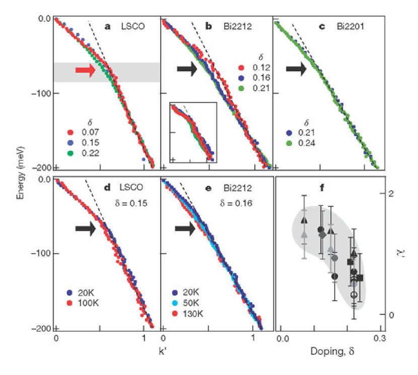
Figure 21: Ubiquitous existence of a kink in the nodal dispersion of various cuprate materialsLanzaraKink . Top panels (a, b, c) plot dispersions along (0, 0)-($\pi$,$\pi$) direction (except for panel b inset, which is off this direction) as a function of the rescaled momentum k’ for different samples and at different doping levels ($\delta$): (a) LSCO at 20 K, (b) Bi2212 in superconducting state at 20 K, and (c) Bi2201 in normal state at 30 K. Dotted lines are guides to the eye. Inset in (b) shows that the kinks in the dispersions off the (0, 0)-($\pi$,$\pi$) direction sharpen upon moving away from the nodal direction. The black arrows indicate the position of the kink in the dispersions. Panels (d) and (e) show the temperature dependence of the dispersions for (d) optimally doped LSCO (x=0.15) and (e) optimally-doped Bi2212, respectively. Panel (f) shows the doping dependence of the effective electron-phonon coupling strength $\lambda$’ along the (0, 0)-($\pi$,$\pi$) direction. Data are shown for LSCO (filled triangles), Nd-doped LSCO (1/8 doping; filled diamonds), Bi2201 (filled squares), and Bi2212 (filled circles in the first Brillouin zone and unfilled circles in the second zone). The different shadings represent data obtained in different experimental runs. Shaded area is a guide to the eye.

While there is a consensus on the data, the exact meaning of the data is still under discussion. The first issue concerns whether the kink in the normal state is related to an energy scale. Valla et al. argued that the system is quantum critical and thus has no energy scale, even though a band renormalization is present in the dataVallaScience . Since their data do not show a sudden change in the scattering rate at the corresponding energy, they attributed the kink in Bi2212 above T_c to the marginal Fermi liquid (MFL) behavior without an energy scalePJohnsonKink . Others believe the existence of energy scale in the normal and superconducting states has a common origin, i.e., coupling of quasiparticles with low-energy collective excitations (bosons)BogdanovKink ; LanzaraKink ; KaminskiKink . The sharp kink structure in dispersion and concomitant existence of a drop in the scattering rate which is becoming increasingly clear with the improvement of signal to noise in the data, as exemplified in underdoped LSCO (x=0.063) in the normal state (Fig. 22b)XJZhouDichotomy , are apparently hard to reconcile with the MFL behavior.

The existence of a well-defined energy scale over an extended temperature range is best seen in Bi2201 compoundLanzaraBi2201 . As shown in Fig.23, the spectra reveal a “peak-dip-hump” structure up to temperatures near 130K, almost ten times the superconducting critical temperature T_c. Such a “peak-dip-hump” structure is very natural in an electron-phonon coupled system, but will not be there if there is no energy scale in the problem as argued by Valla et al.VallaScience .

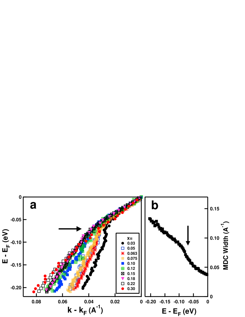
Figure 22: Doping dependence of the nodal electron dynamics in LSCO and universal nodal Fermi velocityXJZhouUniversalVF . (a) Dispersion of LSCO with various doping levels (x=0.03 to 0.30) measured at 20 K along the (0,0)-($\pi$,$\pi$) nodal direction. The arrow indicates the position of kink that separates the dispersion into high-energy and low-energy parts with different slopes. (b). Scattering rate as measured by MDC width (full-width-at-half-maximum, FWHM) of the LSCO (x = 0.063) sample measured at 20 K. The arrow indicates a drop at an energy $\sim$70 meV.

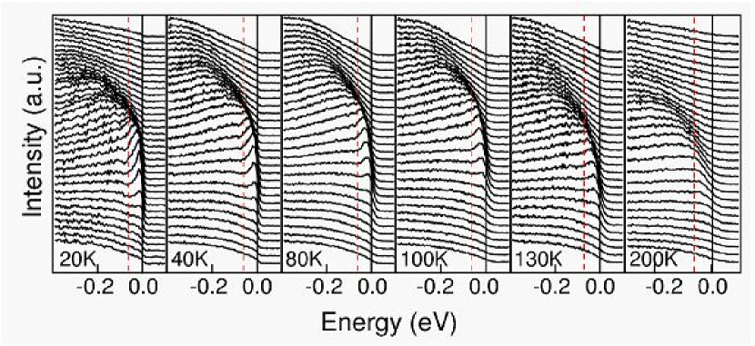
Figure 23: Energy Distribution curves (EDC) in the normal state of underdoped Bi2201 (T_c= 10K) at several temperatures (from 20K to 200K)LanzaraBi2201 . A dip in the EDCs can be clearly observed almost for all the temperatures. The dip position (dotted line) is  60meV and is roughly temperature independent.

A further issue concerns the origin of the bosons involved in the coupling, with a magnetic resonance modeKaminskiKink ; PJohnsonKink and optical phononsLanzaraKink being possible candidates considered. The phonon interpretation is based on the fact that the sudden band renormalization (or “kink”) effect is seen for different cuprate materials, at different temperatures, and at a similar energy scale over the entire doping rangeLanzaraKink . For the nodal kink, the phonon considered in the early work was the half-breathing mode, which shows an anomaly in neutron experimentsPintschoviusBreathingMode ; McQueeneyBreathingMode . Unlike the phonons, which are similar in all cuprates, the magnetic resonance (at correct energy) is observed only in certain materials and only below T_c. The absence of the magnetic mode in LSCO and the appearance of magnetic mode only below T_c in some cuprate materials are not consistent with its being the cause of the universal presence of the kink effect. Whether the magnetic resonance can cause any additional effect is still an active research topicKeeMagneticMode ; AbanovMagneticMode .

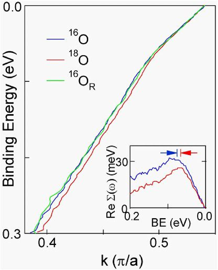
Figure 24: Isotope-induced changes of the nodal dispersionGweonIsotope . The data were taken on optimally doped Bi₂Sr₂CaCu₂O₈ samples (T_c $\sim$ 91 to 92 K) with different oxygen isotopes ¹⁶O and ¹⁸O at T $\sim$ 25 K along the nodal direction. The low energy dispersion is nearly isotope-independent, while the high energy dispersion is isotope-dependent. The effect is reversible by isotope re-substitution (green). Inset shows the real part of the electron self-energy, Re$\Sigma$ , obtained from the dispersion by subtracting a line approximation for the one-electron band $E_{k}$, connecting two points (one at E_F and the other at a 300-meV binding energy) of the ¹⁸O dispersion.

To test the idea of electron-phonon coupling, an isotope exchange experiment has been carried outGweonIsotope . When exchanging ¹⁸O and ¹⁶O in Bi2212, a strong isotope effect has been reported in the nodal dispersions (Fig.24). Surprisingly, however, the isotope effect mainly appears in the high binding energy region above the kink energy; at the lower binding energy near the Fermi level, the effect is minimal. This is quite different from the conventional electron-phonon coupling where isotope substitution will result in a small shift of phonon energy while keeping most of the dispersion intact. The origin of this behavior is still being investigated.

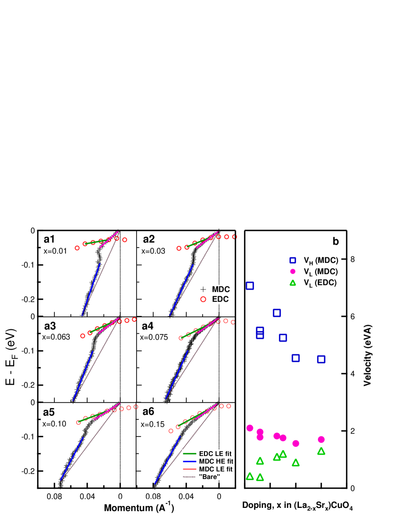
Figure 25: (a). Energy-momentum dispersions for LSCO with different dopings, using both EDC and MDC methodsAndreiEDCMDC . The EDC low-energy velocity is obtained by fitting the EDC dispersion linearly in the intermediate energy range because the data points very close to Fermi level is affected by the Fermi cutoff while the data at higher energy have large uncertainty because the EDCs are broader. The MDC low (high) energy velocity v_H is obtained by fitting MDC dispersion at binding energy 0$\sim$50meV (100 250meV) using a linear line. (b). Low and high-energy velocities as a function of doping obtained from MDC and EDC dispersions.

It is interesting to note in Fig. 22a that the energy scale of the kink also serves as a dividing point where the high and low energy dispersions display different doping dependenceXJZhouUniversalVF . The dispersion in this Figure were obtained by the MDC method. In Fig. 25a, we reproduce some of these MDC-extracted dispersions, but we also plot the dispersion extracted using EDCs by following the EDC peak position. Since the first derivative of the dispersion, $\partial$E/$\partial$k, corresponds to velocity, the dispersions at high binding energy (-0.1$\sim$-0.25eV) and low binding energy (0$\sim$-0.05eV) are fitted by straight lines to quantitatively extract velocities, as plotted in Fig. 25bAndreiEDCMDC .

While nodal data clearly reveal the presence of coupling to collective modes with well-defined energy scale, there are a couple of peculiar behaviors associated with the doping evolution of the nodal dispersion. One obvious anomaly is the difference of low energy velocity obtained from MDC and EDC methods(Fig. 25b). As seen from Fig. 22a and Fig. 25b, the low-energy dispersion and velocity from the MDC method is insensitive to doping over the entire doping range, giving the so-called “universal nodal Fermi velocity” behaviorXJZhouUniversalVF . Similar behavior was also reported in Bi2212PJohnsonKink . However, improved LSCO data where we can resolve a well-defined quasiparticle peak to extract dispersion using EDC method reveal a dichotomy in EDC and MDC derived dispersions, particularly for low doping (Fig. 25), like x=0.01XJZhou001 . This discrepancy between EDC and MDC cannot be reconciled within the conventional el-ph interaction picture, as simulations considering experimental resolutions show.

In terms of conventional electron-phonon coupling, if one considers that the “bare band” does not change with doping but the electron-phonon coupling strength increases with decreasing doping, as it is probably the case for LSCO, one would expect that the low energy dispersion and velocity show strong doping dependence, while the high-energy ones converge. However, one sees that the high-energy velocity is highly doping dependent. Moreover, its trend is anomalous if one takes electron-electron interaction into account. It is known in cuprates that, with decreasing doping, the electron-electron interaction gets stronger. According to conventional wisdom, this would result in a larger effective mass and smaller velocity. However, the doping dependence of the high-energy velocity is just opposite to this expectation, as seen from Fig. 25b.

Therefore, these anomalies indicate a potential deviation from the standard Migdal-Eliashberg theory and the possibility of a complex interplay between electron-electron and electron-phonon interactions. As we discuss later, this phenomenon is a hint of polaronic effect where the traditional analysis fails. Such a polaron effect gets stronger in deeply underdoped system even along the nodal direction. Under such a condition, one needs to use EDC derived dispersion when the peaks are resolved.

IV.3.2 Multiple Modes in the Electron Self-Energy

In conventional superconductors, the successful extraction of the phonon spectral function, or the Eliashberg function, $\alpha^{2}F(\omega)$, from electron tunneling data played a decisive role in cementing the consensus on the phonon-mediated mechanism of superconductivityRowell . For high temperature superconductors, the extraction of the bosonic spectral function can provide fingerprints for more definitive identification of the nature of bosons involved in the coupling.

In principle, the ability to directly measure the dispersion, and therefore, the electron self-energy, would make ARPES the most direct way of extracting the bosonic spectral function. This is because, in metals, the real part of the electron self-energy Re$\Sigma$ is related to the Eliashberg function $\alpha^{2}F(\Omega;\epsilon,\mathbf{\hat{k}})$ by:

$$\mathrm{Re}\Sigma(\mathbf{\hat{k}},\epsilon;T)=\int_{0}^{\infty}d\Omega\alpha^{2}F(\Omega;\epsilon,\mathbf{\hat{k}})K\left(\frac{\epsilon}{kT},\frac{\hbar\Omega}{kT}\right)\,,$$ (15)

where

$$K(y,z)=\int_{-\infty}^{\infty}dx\frac{2z}{x^{2}-z^{2}}f(x+y)\,,$$ (16)

with $f(x)$ being the Fermi distribution function. Such a relation can be extended to any electron-boson coupling system and the function $\alpha^{2}F(\omega)$ then describes the underlying bosonic spectral function. We note that the form of $\mathrm{Re}\Sigma(\mathbf{\hat{k}},\epsilon;T)$ (Eq. 15) can be derived by taking the Kramers-Kronig transformation of $\mathrm{Im}\Sigma$ for the normal state as shown above (Eq. 12). Unfortunately, given that the experimental data inevitably have noise, the traditional least-square method to invert an integral problem is mathematically unstable.

Very recently, Shi et al. have made an important advance in extracting the Eliashberg function from ARPES data by employing the maximum entropy method (MEM) and successfully applied the method to Be surface statesJRShiMEM . The MEM approachJRShiMEM is advantageous over the least squares method in that: (i) It treats the bosonic spectral function to be extracted as a probability function and tries to obtain the most probable one. (ii) More importantly, it is a natural way to incorporate the priori knowledge as a constraint into the fitting process. In practice, to achieve an unbiased interpretation of data, only a few basic physical constraints to the bosonic spectral function are imposed: (a) It is positive. (b) It vanishes at the limit $\omega$$\rightarrow$0. (c) It vanishes above the maximum energy of the self-energy features. As shown in the case of Be surface state, this method is robust in extracting the Eliasberg functionJRShiMEM .

Initial efforts have been made to extend this approach to underdoped LSCO and evidence for electron coupling to several phonon modes has been revealedXJZhouMultipleMode . As seen from Fig. 26, from both the electron self-energy(Fig. 26a), and the derivative of their fitted curves ((Fig. 26a), one can identify two dominant features near $\sim$ 40 meV and $\sim$60 meV. In addition, two addition modes may also be present near $\sim$25meV and $\sim$75 meVXJZhouMultipleMode . The multiple features in Fig. 26b show marked difference from the magnetic excitation spectra measured in LSCO which is mostly featureless and doping dependentHaydenTranquada . In comparison, they show more resemblance to the phonon density-of-states (DOS), measured from neutron scattering on LSCO (Fig.26c)McQueeneyDOS , in the sense of the number of modes and their positions. This similarity between the extracted fine structure and the measured phonon features favors phonons as the bosons coupling to the electrons. In this case, in addition to the half-breathing mode at 70$\sim$80 meV that we previously considered strongly coupled to electronsLanzaraKink , the present results suggest that several lower energy optical phonons of oxygens are also actively involved. Particularly we note that the mode at $\sim$ 60meV corresponds to the vibration of apical oxygens.

We note that, in order to be able to identify fine structure in the electron self-energy, it is imperative to have both high energy resolution and high statisticsZhouValla . These requirements have made the experiment highly challenging because of the necessity to compromise between two conflicting requirements for the synchrotron light source: high energy resolution and high photon flux. Further improvements in photoemission experiments will likely enable a detailed understanding of the boson modes coupled to electrons, and provide critical information for the pairing mechanism.

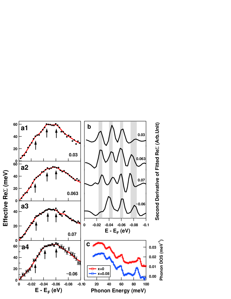
Figure 26: Multiple modes coupling in electron self-energy in LSCOXJZhouMultipleMode . (a).The effective real part of the electron self-energy for LSCO x=0.03 (a1), 0.063 (a2), 0.07 (a3)and $\sim$0.06 (a4) samples. Data (a1-a3) were taken using Scienta 2002 analyzer while data (a4) were taken using Scienta R4000 analyzer. Data (a1-a3) were taking using 10eV pass energy at an energy resolution of $\sim$18meV. Data (a4) were taken a $x\sim$0.06 sample using 5eV pass energy with an energy resolution of $\sim$12meV. For clarity, the error bar is only shown for data (a4) which becomes larger with increasing binding energy. The arrows in the figure mark possible fine structures in the self-energy. The data are fitted using the maximum entropy method (solid red lines). The values of ($\alpha$₁, $\alpha$₂) (the unit of $\alpha$₁ and $\alpha$₂ are eV$\cdot$$\AA$ and eV$\cdot$$\AA$², respectively) for bare band are (-4.25,0) for (a1), (-4.25, 13) for (a2), (-3.7,7) for (a3) and (-4.3, 0) for (a4). (b). The second-order derivative of the calculated Re$\Sigma$. The ruggedness in the curves is due to limited discrete data points. The four shaded areas correspond to energies of (23$\sim$29), (40$\sim$46), (58$\sim$63) and (75$\sim$85) meV where the fine features fall in. ((c) The phonon density of state $F(\omega)$ for LSCO $x=0$ (red) and $x=0.08$ (blue) measured from neutron scatteringMcQueeneyDOS .

One would like to extend this method to the superconducting state, in momentum around the BZ, and to higher temperatures. The superconducting state could, in principle, be achieved by using the BCS dispersion of the quasiparticles rather than the normal state dispersion and is currently under study. However, considering the anisotropy of the el-ph coupling detailed below, the anisotropy of the underlying band structure, and the d-wave superconducting gap, extending the procedure in momentum may be somewhat more difficult. The $\alpha^{2}F(\omega,\varepsilon,{\hat{k}})$ used for the above form of the real part of the self-energy is assumed to be only weakly dependent on the initial energy $\varepsilon$ and momentum $k$ of the electron. But again, one in principle could begin to consider a different form of the calculated Re$\Sigma$ and then apply the MEM method with it instead. Extending the method to higher temperatures, for example $\sim$ 100K for normal state Bi2212 data, may be, however, a limitation that cannot be overcome. The method’s strength is in resolving fine structures due to the phonon density of states. Those fine structures occur predominantly at lower temperatures. At higher temperatures of $\sim$ 100K, the imaginary and real parts of the self energy get broadened on the order of the phonon energy itself. In that case, two or more neighboring phonons would contribute to the electronic renormalization at a given energy, both broadening the fine structures in the data and weakening the resolving power of the method itself. So, while the MEM method can directly extract fine features from ARPES data in agreement with neutron scattering without implicitly assuming a phonon model, it does not have the freedom to incorporate the temperature and momentum dependence needed to describe the ARPES data in both superconducting and normal states, near the vHS and near the node. Both modelling of the data and direct extraction, then, are needed, to gain a complete picture of the mode-coupling features in the data.

IV.3.3 El-Ph Coupling Near the ($\pi$,0) Antinodal Region

The antinodal region refers to the ($\pi$,0) region in the Brillouin zone where the d-wave superconducting gap has a maximum (Fig. 8b). Recently, a low-energy kink was also identified near the ($\pi$,0) antinodal region in Bi2212KaminskiKink ; GromkoAntinodalKink ; KimAntinodalKink ; TCukAntinodalKink . This observation was made possible thanks to the clear resolution of the bi-layer splittingFengBilayersplitting ; ChuangBilayerSplitting ; BogdanovBilayerSplitting . As there are two adjacent CuO₂ planes in a unit cell of Bi2212, these give rise to two Fermi surface sheets from the higher-binding-energy bonding band (B) (thick red curves in Fig. 27c) and the lower-binding- energy antibonding band (A) (thick black curves in Fig. 27c).

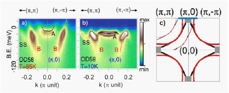
Figure 27: Antinodal kink near ($\pi$,0) in a heavily overdoped Bi2212 sample (T_c$\sim$58 K). (a) Normal-state data (T=85 K) near the antinodal region. (b) Superconducting-state data from the same sample at 10 K, showing the emergence of a dispersion kink in the bilayer split-B band. The B band dispersions (red curves) were determined by fitting MDC peak positions. The black dots represent A band EDC peak positions. (c) Brillouin zone with bonding band B (thick red) and antibonding band A (thick black) Fermi surfaces, as well as momentum-cut locations for panels (a) and (b) (blue bars). The two sets of thin curves are replicas of Fermi surface originating from the superstructure in Bi2212.

Consider a cut along ($\pi$,$\pi$)-(-$\pi$,$\pi$) across ($\pi$,0) in Bi2212, both above T_c (Fig. 27a) and below T_c (Fig. 27b)GromkoAntinodalKink . Superimposed are the dispersion of the bonding band determined from the MDC (red lines) and antibonding band from the EDC (black dots). When the bandwidth is narrow, the applicability of the MDC method in obtaining dispersion becomes questionable so one has to resort to the traditional EDC method. In the normal state, the bonding-band dispersion (Fig. 27a) is nearly linear and featureless in the energy range of interest. Upon cooling to 10 K (Fig. 27b), the dispersion, as well as the near-$E_{F}$ spectral weight, is radically changed. In addition to the opening of a superconducting gap, there is a clear kink in the dispersion around 40 meV.

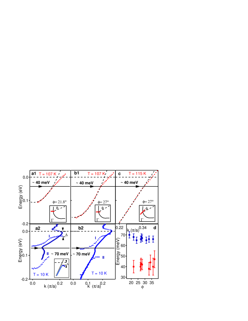
Figure 28: Antinodal kink near ($\pi$,0) in the normal state (a1,b1,c) and superconducting state (a2,b2) in an optimally-doped Bi2212GromkoAntinodalKink . The dispersions in a1, b1, and c were derived by the EDC method; the position of the momentum cuts is labelled in the insets. The red dots are the data; the fit to the curve (black dashed line) below the 40-meV line is a guide to the eye. The dispersions at the same location in the superconducting state (10 K) are shown in (a2) and (b2), which were derived by the MDC method (blue circles). Also plotted in (a2) and (b2) are the peak (blue squares, I) and hump positions (blue squares, II) of the EDCs for comparison. The inset of (a2) shows the expected behavior of a Bogoliubov-type gap opening. The s-like shape below the gap energy is an artifact of the way the MDC method handles the backbend of the Bogoliubov quasiparticle. (d). Kink positions as a function of momentum cuts in the antinodal region.

Gromko et al.GromkoAntinodalKink reported that the antinodal kink effect appears only in the superconducting state and gets stronger with decreasing temperature. Their momentum-dependence measurements show that the kink effect is strong near ($\pi$,0) and weakens dramatically when the momentum moves away from the ($\pi$,0) point. Excluding the possibility that this is a by-product of a superconducting-gap opening, they attributed the antinodal kink to the coupling of electrons to a bosonic excitation, such as a phonon or a collective magnetic excitation. The prime candidate they considered is the magnetic-resonance mode observed in inelastic neutron scattering experiments.

The temperature and momentum dependence identified for a range of doping levels has also led others to attribute the effect to the magnetic resonance KaminskiKink ; KimAntinodalKink . However, there are some inconsistencies with this interpretation: (1) the magnetic resonance has not yet been observed by neutron scattering in such a heavily doped cuprate and (2) the magnetic resonance has little spectral weight, and may be too weak to cause the effect seen by ARPES. Furthermore, the electron-phonon coupling in the early tunneling spectra, such as Pb, appeared prominently only in the superconducting state. The linear MDC-derived dispersion in the normal state of Bi2212 at (pi,0) that Gromko et. al. reportsGromkoAntinodalKink is not conclusive enough proof that the same mode does not couple to the electrons in the normal state. On the other hand, the clear determination of mode-coupling by Gromko et. al. in the anti-nodal region, where the gap is maximum, without the complication of bilayer splitting or superstructure, suggests that the renormalization effects seen by ARPES in the cuprates may indeed by related to the microscopic mechanism of superconductivity.

Cuk et. al. TCukAntinodalKink and Devereaux et. al. DevereauxAntinodalKink have recently proposed a new interpretation of the renormalization effects seen in Bi2212. Specifically, the key observation that prompted them to rule out the magnetic resonance interpretation is the unraveling of the existence of the antinodal kink even in the normal state. This observation was made possible by utilizing the EDC method because the MDC method is not appropriate when the assumed linear approximation of the bare band fails near ($\pi$,0) where the band bottom is close to Fermi level E_F. Figs. 28a1, 28b1, and 28c show dispersions in the normal state of an optimally-doped sample which consistently reveal a  40 meV energy scale that has eluded detection previously. Upon entering the superconducting state, the energy scale shifts to 70meV consistent with a gap opening of 35$\sim$40 meV. This coupling is also found to be more extended in a Brillouin zone than previously reportedGromkoAntinodalKink . In Fig. 30, we show data from the optimally-doped Bi2212 sample for a large portion of the BZ in the superconducting stateTCukAntinodalKink . The renormalization occurs at 70 meV throughout the BZ and increases in strength from the nodal to anti-nodal points. Similar behaviors are also noted by othersKaminskiKink (Fig. 31). The increase in coupling strength can be seen in the following ways: Near ($\pi$,0), the band breaks up into two bands (peak and hump) as seen in Fig. 30a2 and a3. For cuts taken in the (0,0) - ($\pi$, $\pi$) direction, the band dispersion is steeper and the effects of mode-coupling, though significant, are less pronounced.

It is quite natural that phonon modes of different origin and energy preferentially couple to electrons in certain k-space regions. While the detection of multiple modes in the normal state of LSCO(XJZhouMultipleMode suggests that several phonons may be involved, only one has the correct energy and momentum dependence to understand the prominent signature seen in the superconducting state. This new interpretationTCukAntinodalKink attributes the renormalization seen in the superconducting state to the “bond-buckling” B_1g phonon mode involving the out-of-plane, out-of-phase motion of the in-plane oxygens. The bond-buckling phonon is observed at 35 meV in the B_1g polarization of Raman scattering on an optimally doped sample, the same channel in which the $\sim$ 35-40 meV d-wave superconducting gap shows up Friedl ; Devereaux3 ; Opel . Applying simple symmetry considerations and kinematic constraints, it is found that this B_1g buckling mode involves small momentum transfers and couples strongly to electronic states near the antinodeDevereauxAntinodalKink . In contrast, the in-plane Cu-O breathing modes involve large momentum transfers and couple strongly to nodal electronic states. Band renormalization effects are also found to be strongest in the superconducting state near the antinode, in full agreement with angle-resolved photoemission spectroscopy data (Fig. 29). The dramatic temperature dependence stems from a substantial change in the electronic occupation distribution and the opening of the superconducting gapTCukAntinodalKink ; DevereauxAntinodalKink . It is important to note that the electron-phonon coupling, especially the one with B_1g phonon, explains the temperature and momentum dependence of the self-energy effects that were taken as key evidence to support the magnetic resonance interpretation of the data. Compounded with the findings that cannot be explained by the magnetic resonance as discussed earlier, this development makes the phonon interpretation of the kink effect self-contained.

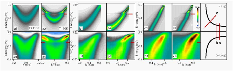
Figure 29: Comparison between the calculated and measured spectral function in Bi2212 including electron-phonon coupling for three different momentum cuts (a, b, c) through the Brillouin zone. (a1,b1,c1) and (a2,b2,c2) show the calculated spectral functions in the normal and superconducting states, respectivelyDevereauxAntinodalKink . The measured spectral functions are shown in (a3,b3,c3) for the normal state and in (a4,b4,c4) for the superconducting state. The corresponding momentum cuts a, b, and c are shown in the rightmost panel. The red markers in the superconducting state indicate 70 meV. The simulation includes B1g oxygen buckling mode and half-breathing mode.

IV.3.4 Anisotropic El-Ph Coupling

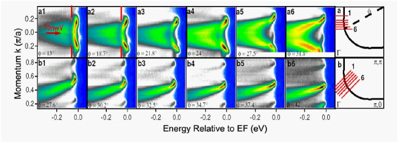
Figure 30: Anisotropic electron-boson coupling in Bi2212TCukAntinodalKink . Image plots in (a1-a6) and (b1-b6) are cuts taken parallel to (0, $\pi$)-($\pi$, $\pi$) and (0, 0)-($\pi$, $\pi$) respectively at the locations indicated in the Brillouin zone ((a) and (b)) at 15 K for an optimally doped sample (T_c = 94 K).

The full Migdal-Eliashberg-based calculation consists of a tight-binding band structure and el-ph coupling to the breathing mode as well as the B_1g bond-buckling mode and is based on an earlier calculation TDevereaux2 . The electron-phonon coupling vertex $g(k,q)$, where $k$ represents the initial momentum of the electron and $q$ the momentum of the phonon is determined on the basis of the oxygen displacements for each mode in the presence of the underlying band-structure. In the case of the breathing mode, the in-plane displacements of the oxygen modulate the CuO₂ nearest neighbor hopping integral as well as the site energies. In the case of the bond-buckling mode, one must suppose that the mirror plane symmetry across the CuO₂ plane is broken in order for electrons to couple linearly to phonons. The mirror plane symmetry can be broken by the presence of a crystal field perpendicular to the plane, tilting of the Cu-O octahedral, static in-plane buckling, or may be dynamically generated.

Figure 31: Momentum dependence of photoemission data in optimally-doped Bi2212KaminskiKink . Left panels: Photoemission data in the normal state (T=140 K) along selected cuts parallel to M($\pi$,0)-Y($\pi$,$\pi$). EDC peak positions are indicated by crosses. Middle panels: Photoemission data in the superconducting state (T=40 K) at the same cuts as for left panels. Crosses indicate positions of broad high energy peaks, dots sharp low energy peaks. Right panels: EDCs at locations marked by the vertical lines in the middle panels.

The $g_{B_{1g}}(k,q)$ form factor leads to preferential $q\sim 2k_{f}$ scattering between the parallel pieces of Fermi surface in the anti-nodal region, as shown in Fig. 32 depicting $g(k,k^{\prime})$ for the buckling mode (where $k^{\prime}=k-q$) for an electron initially at the anti-node ($k_{AN}$; upper-left) and for an electron initially at the node ($k_{N}$; bottom-left). This coupling anisotropy partially accounts for the strong manifestation of electron-phonon coupling in the anti-nodal region where one sees a break up into two bands. The breathing mode, in contrast, modulates the hopping integral and has a form factor, $g_{br}(k,q)$, that leads to preferential scattering for large $q$ and couples opposing nodal states. This coupling anisotropy then accounts for the 70 meV energy scale seen most prominently in a narrow $k$-space region near the nodal direction in the normal state of LSCO. Fig. 32 also shows that the magnitude of the electron-phonon vertex is largest for an electron initially sitting at the node, $k_{N}$, that scatters to the opposing nodal state. For more details on this calculation, see Devereaux et. al. DevereauxAntinodalKink .

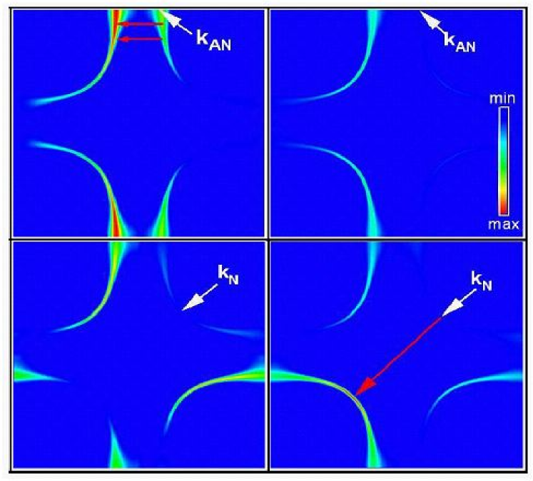
Figure 32: Plots of the electron-phonon coupling $\mid g(\textbf{k},\textbf{q})\mid^{2}$ for initial k and scattered $\bf{k^{\prime}=k-q}$ states on the Fermi surface for the buckling mode (left panels) and breathing mode (right panels) for initial fermion k at an anti-nodal (top panels) and nodal (bottom panels) point on the Fermi surface, as indicated by the arrows. The red/blue color indicates the maximum/minimum of the el-ph coupling vertex in the BZ for each phononDevereauxAntinodalKink .

The anisotropy of the mode-coupling in both the superconducting state data and the calculation is peculiar to the cuprates. Such a strong anisotropy in the electron-phonon coupling is not traditionally expected. In cuprates, the sources of the anisotropy are: 1) an electron-phonon vertex for the B_1g bond-buckling mode and the breathing mode that depends both on the electron momentum $k$ as well as the phonon momentum $q$. This comes from a preferential scattering in the Brillouin zone, in which nodal states couple to other nodal states and anti-nodal states to other anti-nodal states. 2) a strongly anisotropic electronic band structure characterized by a van Hove Singularity (vHS) at ($\pi$,0). In the anti-nodal region and along the $(\pi,0)-(\pi,\pi)$ direction in which 2$k_{F}$ scattering is preferred, the bands are narrow, giving rise to a larger electronic density of states near the phonon energy and therefore a stronger manifestation of electron-phonon coupling. 3) a d-wave superconducting gap and 4) a collusion of energy scales in the anti-nodal region that resonate to enhance the above effects—the vHS at $\sim$ 35meV in the tight-binding model that best fits the data, the maximum d-wave gap at $\sim$ 35meV, and the bond-buckling phonon energy at $\sim$ 35meV. All these three factors collide to give the anisotropy of the mode-coupling behavior in the superconducting and normal states. For a detailed look at how each plays a role in the agreement with the data, please see Cuk et. al. TCukAntinodalKink . The coincidence of energy scales, along with the dominance of the renormalization near the anti-node, indicates the potential importance of the B_1g phonon to the pairing mechanism, which is consistent with some theory on the B_1g phononJepsen ; KAMuller ; Scalapino2 ; Nazarenko but remains to be investigated.

The cuprates provide an excellent platform on which to study anisotropic electron-phonon interaction. In one material, such as optimally doped Bi2212, the effective coupling can span $\lambda$ of order $\sim$1 at the node to 3 at the anti-node (Fig.33)TCukAntinodalKink ; DevereauxAntinodalKink . In addition to the large variation of coupling strength, there is a strong variation in the kinematic considerations for electron-phonon coupling. In the nodal direction, the band bottom is far from the relevant phonon energy scales. However, at the anti-node, the relevant phonon frequencies approach the bandwidth. Indeed the approximation of Migdal, in which higher order vertex corrections to the el-ph coupling are neglected due to the smallness of ($\lambda*\Omega_{{}_{ph}}/E_{F}$), may be breaking down in the anti-nodal region. Non-adiabatic effect beyond the Migdal approximation have been considered and are under continuing study Pietrano .

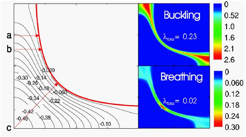
Figure 33: Plots of the electron-phonon coupling $\lambda_{\bf k}$ in the first quadrant of the BZ for the buckling mode (right top panel) and breathing mode (right bottom panel). The color scale is shown on the right for each phonon. The left panel shows energy contours for the band structure usedDevereauxAntinodalKink .

IV.4 Polaronic Behavior

IV.4.1 Polaronic Behavior in Parent Compounds

The parent compounds of the cuprate superconductors, being antiferromagnetic Mott insulators, provide an ideal testing ground for investigating the dynamics of one hole in an antiferromagnetic background. Indeed, many theories have been formed and tested by ARPES on a number of compounds, among them are Sr₂CuO₂Cl₂WellsSCOC ; LaRosa ; CKimSCOC ; Pothuizen ; RonningUniver , Ca₂CuO₂Cl₂RonningScience ; RonningUniver ; RonningPRB ; KShenPolaron ; KShenScience , Nd₂CuO₄ArmitageNCCO , and La₂CuO₄InoSITrans ; YoshidaArc ; RoschLCO . However, several aspects of the data can only be explained by invoking polaron physics, as we will now discuss.

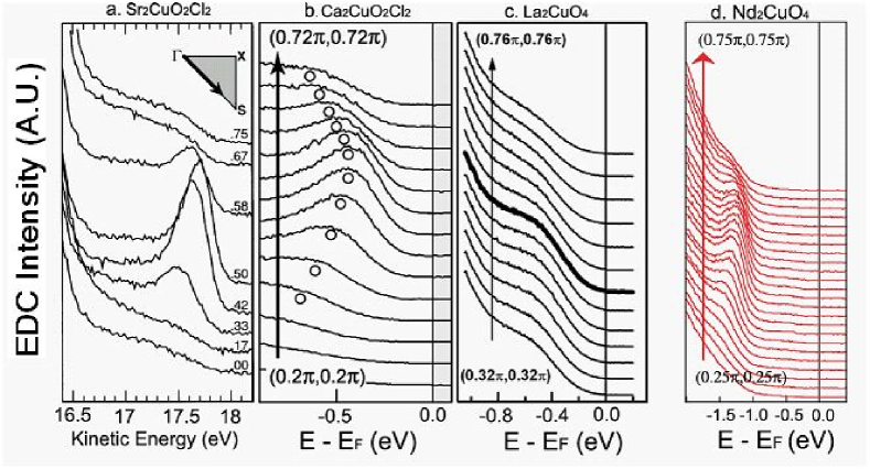
Figure 34: (a). Photoemission spectra along the (0,0) and ($\pi$,$\pi$) direction in Sr₂CuO₂Cl₂WellsSCOC ; CKimSCOC , Ca₂CuO₂Cl₂RonningPRB ; KShenPolaron , La₂CuO₄YoshidaArc ; RoschLCO and Nd₂CuO₄ArmitageNCCO .

The ARPES measurements on SCOCWellsSCOC ; CKimSCOC and CCOCRonningPRB ; KShenPolaron give essentially similar results. As seen in Fig. 34a and 34b, along the (0,0)-($\pi$,$\pi$) direction, the lowest energy feature disperses toward lower binding energy with increasing momentum, reaches its lowest binding energy position near ($\pi$/2,$\pi$/2) where it becomes sharpest in its lineshape, and then suddenly loses intensity after passing ($\pi$/2,$\pi$/2) and bends back to high binding energy. This behavior can be more clearly seen in the image plot of Fig. 35aRonningPRB where the “band” breaks into two branches. The lowest binding energy feature shows a dispersion of $\sim$0.35 eV while an additional band at high binding energy (Fig. 35a) is very close to the unrenormalized band predicted by band theoryRonningPRB . The dispersion of low binding-energy band along the (0,0)-($\pi$,$\pi$) direction and other high symmetry directions are shown in Fig. 35b by keeping track of the EDC peak positionTTohyama . The total dispersion of the peak is $\sim$0.35eV. This is in contrast to the predictions of one-electron band calculations which gives an occupied band width of $\sim$ 1.5 eV and total bandwidth of $\sim$3.5 eVCCOCBandCal . Nevertheless, it is consistent with the calculations from the t-J model where the predicted occupied bandwidth is $\sim$2.2JZPLiu ; DagottoRMP . This indicates that the dynamics of one-hole in an antiferromagnetic background is renormalized from scale $t$ to scale $J$.

Figure 35: (a). Intensity plot of ARPES data as functions of the binding energy and momentum for Ca₂CuO₂Cl₂ along the $\Gamma$(0,0)-($\pi$,$\pi$) directionRonningPRB . The data was symmetrized around the $\Gamma$ point. Also shown on the plot are the dispersions obtained by following the peak positions of the MDCs (solid line) and the EDCs (circle and triangles). The results are compared with the shifted dispersion from the LDA calculation (dashed line). (b) Energy dispersion of quasiparticle for insulating Sr₂CuO₂Cl₂ measured from the top of the band. Experimental data are taken from WellsSCOC (open circles), LaRosa (open triangles) and CKimSCOC (open squares). Solid circles: the results of the self-consistent Born approximation (SCBA) for the t$-$t${}^{{}^{\prime}}$$-$t^"$-$J model with t = 0.35 eV, $t^{{}^{\prime}}$ = -0.12 eV, $t^{"}$ = 0.08 eV and J = 0.14 eV. The solid lines are obtained by fitting the SCBA data to a dispersion relation given by E₀(k) + E₁(k), being t${}^{{}^{\prime}}_{eff}$ = -0.038 eV and t${}^{"}_{eff}$ = 0.022 eV. The dashed line along the ($\pi$, 0) C(0,$\pi$) direction represents the spinon dispersion from LaughlinSCOC .

While the t-J model and experiments show agreement along the (0,0)-($\pi$,$\pi$) direction, there are discrepancies along other directions, such as the (0,0)-($\pi$,0) and (0,$\pi$)-($\pi$/2,$\pi$/2)-($\pi$,0) directionsWellsSCOC . The later intensive theoretical effort resolved this issue by incorporating the hopping to the second (t${}^{{}^{\prime}}$) and third (t^") nearest-neighborsSCOCExttJ . More precise calculations of the dispersion in the t$-$t${}^{{}^{\prime}}$$-$t^"$-$J model are performed by using a self-consistent Born approximation (SCBA)SCB . These calculations show a satisfactory agreement with experimentally derived dispersion, as shown in Fig. 35bTTohyama .

However, there remain a few prominent puzzles related to the interpretation of the photoemission data in undoped parent compoundsKShenPolaron . The first prominent issue is the linewidth of the peak near ($\pi$/2,$\pi$/2). As highlighted in Fig. 36a, the width of the sharpest peak near ($\pi$/2,$\pi$/2) is $\sim$300 meV which is comparable with the entire occupied bandwidth $2J\approx$350 meV KShenPolaron . This is much broader than that from t-J model calculations and too broad to be considered as a coherent quasiparticle peak for which the quasiparticle peak is basically resolution limited, as exemplified by the data on Sr₂RuO₄ in Fig. 36a. An early attempt interpreted this anomalously large linewidth to additional interaction with a non$-$magnetic boson bath of excitations, such as phononsPothuizen . But this interpretation meets with difficulty in explaining little renormalization in the dispersion from this “extra interaction” because dispersion and linewidth are closely related. A diagrammatic quantum Monte Carlo studyAMtJPolaron showed that this problem can be resolved by considering the polaron effect in the t-J model. Namely the dispersion for the center of mass of the spectral function obeys that of the pure t-J model, while the lineshape is strongly modified. The details of this will be given below.

Another unresolved issue is the chemical potential $\mu$. For an insulator, $\mu$ is not well defined, and may be pinned by surface defects or impurities and will vary between different samples. If one considers that the peak A in Fig.36a represents a quasiparticle peak, one would expect the chemical potential to vary anywhere above the top of this valence band. However, the experimental chemical potential clearly sets a lower bound that is $\sim$0.45eV apart from the peak A (Fig. 36b)KShenPolaron . Shen et al.KShenPolaron invented a new method to determine the chemical potential using both the energy of the non-hybridized oxygen orbital and the detailed line-shape of Na-CCOC.

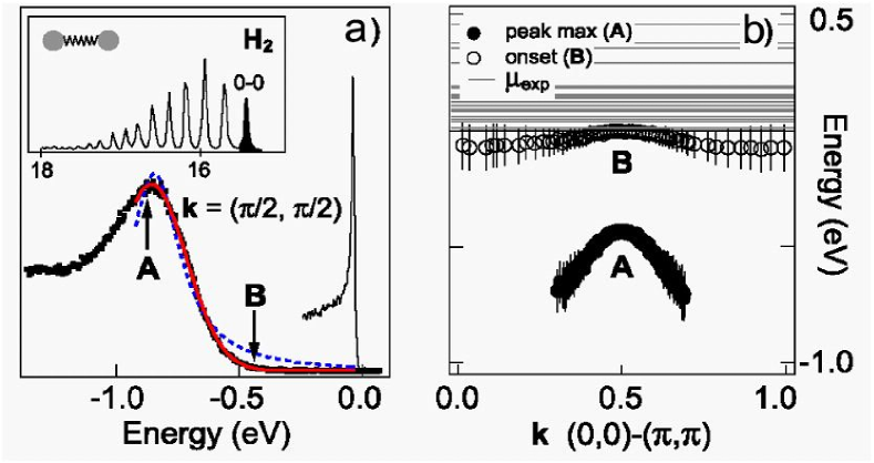
Figure 36: (a) Photoemision spectrum of Ca₂CuO₂Cl₂ at k=($\pi$,$\pi$) with fits to a Lorentzian spectral function (dashed) and Gaussian (red or gray)KShenPolaron . A and B denote the peak maximum and the onset of spectral weight, respectively. Comparison with Fermi-liquid system Sr₂RuO₄ is shown (thin black). Upper inset shows photoemission spectra from H₂HydrogenFC . (c) Dispersion of A and B along (0,0)-($\pi$,$\pi$), along with experimental values for the chemical potential $\mu$ (lines).

The resolution of these discrepancies between experiment and expectation leads to identifying polaron physics as responsible for the bulk of the lineshape in underdoped cuprates. In fact, the photoemission spectra in the underdoped cuprates resemble the Frank-Condon effect seen in photoemission spectra of molecules such as H₂HydrogenFC (inset of Fig. 36), where only the “0-0” peak (filled black) represents the H final state with no excited vibrations and comprises only $\sim$10$\%$ of the total intensity. In the solid state, this “0-0” would correspond to the quasiparticle or the coherent part of the spectral function, A_coh, whereas the excited states comprise the incoherent part, A_inc. This behavior is reminiscent of polarons, and such models have been invoked in systems where strong couplings are presentARPESPolaron . In this picture, in the undoped compound, the true QP (B) is hidden within the tail of spectral intensity, with a quasiparticle residue $Z$ vanishingly small, while feature A is simply incoherent weight associated with shake-off excitations.

From the viewpoint of polaron physics, the cuprates offer a unique and first opportunity to compare experimental spectra with theory in detail. The single hole interacts both with magnons and phonons. The hole-magnon interaction has been successfully analyzed in terms of the self-consistent Born approximaitonSCB . The success of the Born approximation results from a “saturation” effect; namely the single spin 1/2 can flip only once, and hence magnon clouds do not become large enough to induce the self-trapping transition to the small polaron. On the other hand, phonon clouds can be larger and larger as the coupling constant $g$ increases and can lead to a self-trapping transition. The t-J model coupled to phonons in the polaronic regime has illuminated one-hole dynamics in the parent compound in the following wayAMtJPolaron . (1). With increasing electron-phonon coupling strength, the spectral function experiences a transition from weak-coupling, to intermediate coupling, and to strong-coupling regimes. (2). In the strong coupling regime, the spectral function consists a ground state resonance (as indicated by vertical arrows) with vanishing intensity and a broad peak denoted as “coherent C”, as shown in Fig.37a. (3). The broad peak C shows strong momentum dependence while the lowest state is dispersionless. These results are in good correspondence to experimental observations. The most surprising result is that the broad resonance has the momentum dependence of the t-J model without coupling to phonons (shown in Fig. 37b). In the Franck-Condon effect for molecules a similar result occurs. The center of the shake-off band corresponds to the hole motion in the background of the frozen lattice configuration, i.e. the dispersion of the hole remains that of the non-interacting limit, while the line-width broadens. A more elaborated analytic treatment of the t-J polaron model in the Franck-Condon approximationGunnEur successfully reproduced this Monte Carlo results. The calculated spectral function line-shape most consistent with experiment has a $\lambda\cong 0.9-1.3$, well within the strong-coupling, small-polaron regime. Recent realistic shell model calculationRoschLCO also concluded $\lambda=1.2$ for La₂CuO₄.

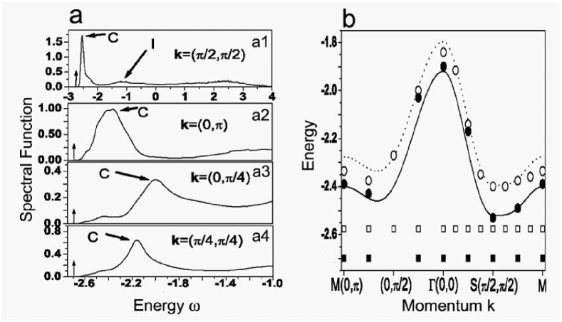
Figure 37: (a). Calculated hole spectral function in ground state at $J/t=0.3$ for different momentaAMtJPolaron . (a1) Full energy range for $k=(\pi/2,\pi/2)$. (a2)$-$(a4) Low energy part for different momenta. Slanted arrows show broad peaks which can be interpreted in ARPES spectra as “coherent” (C) and incoherent (I) part. Vertical arrows indicate position of ground state resonance which is not seen in the vertical scale of the figure. (b). Dispersion of resonance energies at $J/t=0.3$. Broad resonance (filled circles) and lowest polaron resonance (filled squares) at $g=0.231125$; third broad resonance (open circles) and lowest polaron resonance (open squares) at g=0.2. The solid curves are dispersions of a hole in the pure t-J model at $J/t=0.3$.

In La₂CuO₄, a broad feature near -0.5eV (Fig. 38) was identified as the lower Hubbard bandInoSITrans ; YoshidaArc . The electron-phonon coupling strength, calculated using a shell model, puts La₂CuO₄ in the polaron regime, similar to Ca₂CuO₂Cl₂. In this picture, the -0.5eV feature corresponds to the phonon side-band while the real quasiparticle residue is very weak. As shown in Fig. 38, the calculated spectral function agrees well with the measured dataRoschLCO .

Figure 38: Polarons in La₂CuO₄RoschLCO . Calculated ARPES spectra for the undoped La₂CuO₄ system at T=0 for different $\bf{k}$ normalized to the height of the phonon side band. The lower abscissa shows binding energies (BE) and the upper abscissa the energies of the final states corresponding to the spectral features. The inset shows the dependence of the width of the phonon side band on its binding energy. The width of the $(0,0)$ spectrum is poorly defined and not shown.

IV.4.2 Doping Dependence: From Z$\sim$0 Polaron to Finite Z Quasiparticles

We next turn to the question of how the small polaron state evolves as a function of doping, connecting to the Migdal-Eliashberg regime discussed in section C. There are two possible ways to dope the Mott insulator, schematically shown in Fig. 10cSUchidaGap ; Veenendaal : (1). Upon doping, the chemical potential shifts to the top of the valence band for hole doping (Fig. 10c3) or to the bottom of the conduction band for electron doping (Fig. 10c4). (2).The chemical potential is pinned inside the charge transfer gap. Upon doping, new states will form inside the gap (Fig. 10c5).

Recent ARPES measurements on lightly-doped (La_2-xSr_x)CuO₄ compounds provide a good window to look into this issue. As shown in Fig. 39a and 39e, for undoped La₂CuO₄, the main feature is the broad peak near -0.5 eV which exhibits weak dispersionYoshidaArc . There is also little spectral weight present near the Fermi level. However, upon only a doping of $x=0.03$, the electronic structure undergoes a dramatic change. A new dispersive band near the Fermi level develops along the (0,0)-($\pi$,$\pi$) nodal direction(Fig. 39e, right panel), while along the (0,0)-($\pi$,0) direction a saddle band residing -0.2eV below the fermi level develops. Even for more lightly-doped samples, such as $x=0.01$, new states near the Fermi level are createdXJZhou001 . Note that, for these lightly-doped samples, the original -0.5 eV remains, although with weakened spectral weight (Fig. 39d). So, the -0.5eV peak and the new dispersive band coexist at doping levels close to the parent compounds.

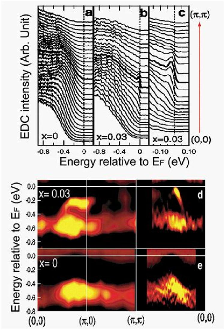
Figure 39: Creation of nodal quasiparticles in lightly-doped LSCOYoshidaArc . ARPES spectra for LSCO with $x$=0 and $x$=0.03. Panels a and b are EDC’s along the nodal direction (0,0)-($\pi,\pi$) in the second Brillouin zone (BZ). The spectra for $x$ = 0.03 are plotted on an expanded scale in panel c. Panels d and e represent energy dispersions deduced from the second derivative of the EDC’s.

The systematic evolution of the photoemission spectra near the nodal and antinodal regions with doping in LSCO is shown in Fig. 40a and bYoshidaArc . The nodal quasiparticle weight, Z_QP, integrated over a small energy window near the Fermi level, is shown in Fig. 40c. In the underdoped region, it increases with increasing doping nearly linearly, and no abrupt change occurs near the nonsuperconductor-superconductor transition at $x\sim$0.05.

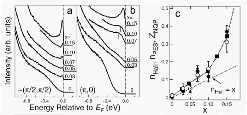
Figure 40: ARPES spectra at $\mathbf{k}=\mathbf{k}_{\mathrm{F}}$ in the nodal direction in the second BZ (a) and those at ($\pi,0$)(b) for various doping levelsYoshidaArc . (c).Doping dependence of the nodal QP spectral weight, $Z_{\rm NQP}$, and the spectral weight integrated at $E_{\mathrm{F}}$ over the entire second Brillouin zone, $n_{\rm PES}$YoshidaArc . They show similar doping dependence to the hole concentration evaluated from Hall coefficient ($n_{\rm Hall}$) TakagiHall .

(Ca_2-xNa_x)CuO₂Cl₂ (Na$-$CCOC) is another ideal system to address the doping evolution of the electronic structure. The precise measurement of the chemical potential (Fig. 41a), in conjunction with the identification of polaron physics in the under-doped compounds, provides a globally consistent picture of the doping evolution of the cupratesKShenPolaron . Instead of measuring the chemical potential with deep core level spectroscopy (the usual method)InoChemPotential , one utilizes orbitals in the valence band at lower energies(Fig. 41a and b). The measured chemical shift, $\Delta$$\mu$, exhibits a strong doping dependence, $\partial$$\mu$/$\partial$x=-1.8$\pm$0.5 eV/hole, comparable to the band structure estimation ($\sim$-1.3 eV/hole) (Fig. 41c).

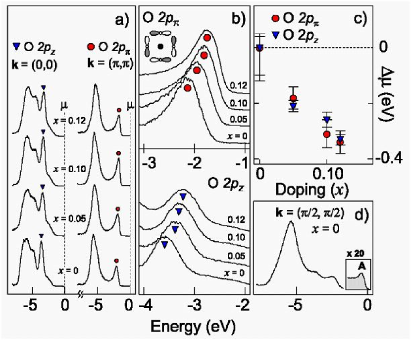
Figure 41: Chemical potential shift in Na-CCOCKShenPolaron . (a) Valence band spectra for x=0, 0.05, 0.10, and 0.12 compositions at k=(0,0) and ($\pi$,$\pi$). O 2p_z and O 2p_pi states are marked by triangles and circles, respectively. (b) Shifts of the O 2p_z and O 2p_pi peaks shown on an expanded scale. (c) Doping dependence of chemical potential $\Delta$$\mu$ determined from (b). (d) Valence band at k=($\pi$/2,$\pi$/2), showing the lower Hubbard band (A) on an expanded scale.

Figs. 42(a-d) show the doping evolution of the near-E_F EDCs plotted relative to $\mu$₀ of the undoped sample (determined in Fig. 41c). With doping, feature A evolves smoothly into a broad, high energy hump with a backfolded dispersion similar to the parent insulator (symbols), while B shifts downward relative to its position in the un-doped compound. Spectral weight increases with doping at B, and a well-defined peak emerges for the $x=$0.10 and 0.12 samples, resulting in a coherent, low-energy band. The dispersion of the high-energy hump (A), tracked using the local maxima or second derivative of the EDCs, shows little change as a function of doping (Fig. 41e). The lowest energy excitations (feature B, -0.05eV$<$E$<$E_F), tracked using MDC analysis, evolve with doping in such a way that the quasiparticle dispersion ($v_{F}$) and Fermi wave vectors ($k_{F}$) virtually collapse onto a single straight line.

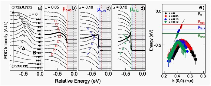
Figure 42: (a-d). EDC spectra of Na-CCOC x=0 (a), 0.05(b), 0.10(c), and 0.12(d) from (0.2$\pi$,0.2$\pi$) to (0.72$\pi$,0.72$\pi$) with hump positions marked by open symbols and the EDC at k_F shown in boldKShenPolaron . Data are plotted on a relative energy scale referenced to the shift in $\mu$ shown in Fig. 41c. (e). Summary of hump (symbols)from Fig. (a-d) and MDC dispersions (lines).

IV.4.3 Doping Evolution of Fermi Surface: Nodal-Antinodal Dichotomy

So far, we have discussed the doping evolution along the nodal direction, and seen that a sharply defined quasiparticle peak develops out of the small weight near the chemical potential in the undoped samples. We now discuss the doping evolution in other directions of the Brillouin zone. Surprisingly, one finds that the coherent peak near the Fermi level in the lightly doped samples is confined to the nodal region, and quickly disappears with momentum around the Brillouin zone. The spectral weight near the Fermi level, confined to the ($\pi$/2,$\pi$/2) nodal region, forms a so-called “Fermi arc”. This dichotomy between nodal and antinodal excitations is shown in Fig. 43XJZhouDichotomy . For the $x=0.063$ sample, which is close to the nonsuperconductor-superconductor transition and therefore heavily underdoped, the spectral weight near Fermi level is mainly concentrated near the nodal region (Fig. 43a). The coherent peaks in the EDCs (Fig. 43c1) near the nodal region disappear as one approaches the anti-nodal region, where the EDCs exhibit a step rather than a peak. The LSCO $x=0.09$ sample exhibits similar behavior(Fig. 43c2). In contrast, for overdoped LSCO such as $x=0.22$ (Fig. 43c3), sharp peaks are observable along the entire Fermi surface. These observations indicate that the electrons near the antinodal region experience additional scattering. Therefore, as shown in Fig. 44, the “Fermi surface” in LSCO evolves from the “Fermi arc” in lightly-doped samples, to a hole-like Fermi surface in underdoped samples, and to an electron-like Fermi surface in overdoped samples (x$>$0.15).

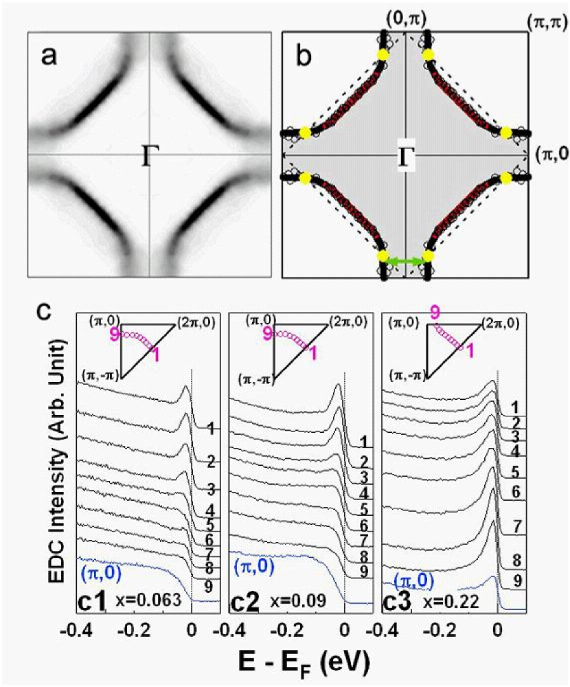
Figure 43: Dichotomy between nodal and antinodal excitations in LSCOXJZhouDichotomy . (a). Spectral weight near a small energy window of Fermi level as a function of $k_{x}$ and $k_{y}$ for LSCO $x=0.063$ sample measured at $\sim$20K. The original data was taken in the second Brillouin zone and converted into the first Brillouin zone and symmetrized under four-fold symmetry. (b). Experimental Fermi surface for LSCO $x=0.063$ sample. The black open circles are obtained from the MDC peak position at $E_{F}$. The solid lines are guides to the eye for the measured Fermi surface. The red lines represent the portion of Fermi surface where one can see quasiparticle peaks. The dotted black line represents the antiferromagnetic Brillouin zone boundary; its intersection with the Fermi surface gives eight hot spots (solid yellow circles) from ($\pi$,$\pi$) magnetic excitations. The double-arrow-ended green line represents a nesting vector between the antinodal part of the Fermi surface (c). EDCs on Fermi surface for LSCO $x=0.063$ (c1), 0.09 (c2), and 0.22 (c3) samples. All samples are measured at $\sim$20 K. The corresponding momentum position is marked in the upper inset of each panel. Also included are the spectra at ($\pi$,0) points, colored as blue.

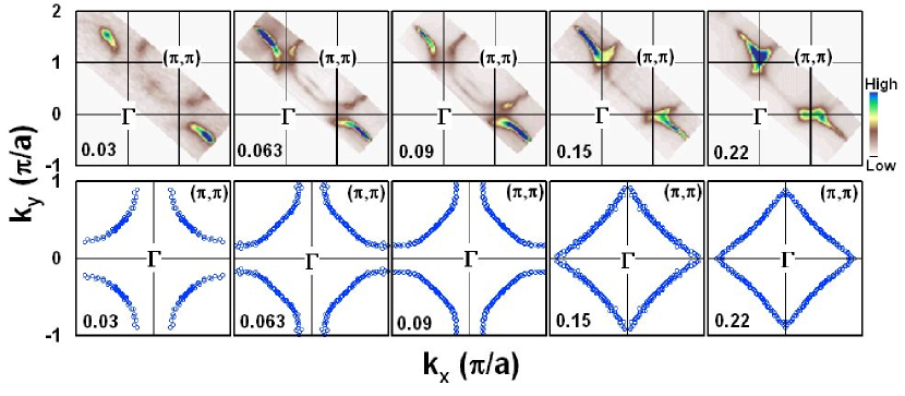
Figure 44: Doping evolution of underlying ”Fermi surface” in (La_2-xSr_x)CuO₄YoshidaArc ; XJZhouDichotomy ; XJZhouDuality ; Yoshida22 . The data were measured at a temperature of $\sim$20K.

The evolution of electronic structure with doping in (Ca_2-xNa_x)CuO₂Cl₂ exhibits marked resemblance to that in (La_2-xSr_x)CuO₄KShenScience . As summarized in Fig. 45, at low doping, the quasiparticle weight is again confined to the nodal region and the weight in the quasiparticle peak, Z_qp, increases with increasing doping, consistent with LSCO. In the Na$-$CCOC system, recent scanning tunneling microscopy (STM) work has revealed a real space pattern of 4a₀ $\times$ 4a₀ two-dimensional charge orderingCCOCSTM . In momentum space, as seen from Fig. 46, strong Fermi surface nesting exists in Na$-$CCOC with a nesting vector insensitive to doping close to 2$\ast$$\pi$/4 that may account for the broad near-E_F spectra in the anti-nodal region. In LSCO, neutron scattering has also indicated the existence of dynamic stripesTranquadaStripe . These similarities suggest an intrinsic commonality between the low-lying excitations across different cuprate families and may imply a generic microscopic origin for these essential nodal states irrespective of other ordering tendencies. At very low doping levels, the nodal excitations should entirely dominate the transport properties, consistent with the high-temperature metallic tendencies observed in very lightly doped cupratesAndoMetalLSCO . Thus any microscopic models of charge ordering must simultaneously explain and incorporate the existence of coherent nodal states and broad antinodal excitations.

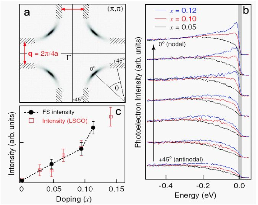
Figure 45: Dichotomy between nodal and antinodal excitations in Na-CCOCKShenScience . (a). Schematic of the low-lying spectral intensity for (Ca_2-xNa_x)CuO₂Cl₂ (x=0.10). The hatched regions show the nested portions of Fermi surface, and the Fermi surface angle is defined in the lower right quadrant. (b). EDCs taken at equal increments along the FS contour from the nodal direction (top) to the antinodal region (bottom) for x=0.05, 0.10, and 0.12 at a temperature of 15 K. (c). The doping evolution of the low-lying spectral weight (circles), along with corresponding data from La_2CxSr_xCuO₄ (squares), with the error bars representing the uncertainty in integrated weight as well as sample-to-sample variations.

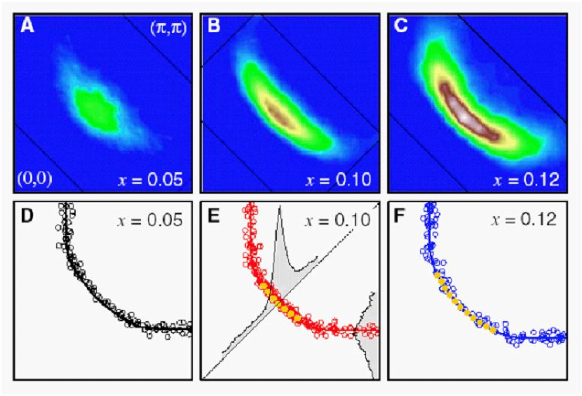
Figure 46: Doping evolution of “Fermi surface” in Na-CCOCKShenScience . (A to C) The momentum distribution of spectral weight within a $\pm$10-meV window around E_F for x=0.05, 0.10, and 0.12 in one quadrant of the first Brillouin zone. Data were taken at 15 K and symmetrized along the (0,0)- ($\pi$,$\pi$) line. The data acquisition range is shown within the black lines. The FS contours shown in (D to F) were compiled from more than four samples for each composition with different photon energies and photon polarizations. Data from these samples constitute the individual points; the best fit is shown as a solid line. The region in which a low-energy peak was typically observed is marked by gold circles. The gray shaded areas in (E) represent the momentum distribution of intensity at E_F$\pm$10 meV along the (0,0)-($\pi$,$\pi$) and ($\pi$,0)-($\pi$,$\pi$) high-symmetry directions.

The nodal-antinodal dichotomy of quasiparticle dynamics in the normal state also exists in Bi2212ShenSchrieffer . A number of possible mechanisms have been proposed to account for the antinodal spectral broadening in the normal state. A prime candidate is the ($\pi$,$\pi$) magnetic excitations observed in various cupratesResonanceModeYBCO ; ResonanceModeBi2212 ; RMHeTl2201 . As schematically shown in Fig. 43b, this excitation will give rise to “hot spots” on the Fermi surface that can be connected by ($\pi$,$\pi$) momentum transfer. Electrons around these hot spots experience additional scattering from the ($\pi$,$\pi$) magnetic scattering. The same mechanism has also been proposed for (Nd_2-xCe_x)CuO₄ for which the spectral broadening is localized to the expected “hot spot”NCCOHotSpot . However, in LSCO, the same magnetic response, magnetic resonance mode, is not observed. Instead, incommensurate magnetic peaks are observed at low energy (below 15 meV)TranquadaStripe , which broaden rapidly with increasing energy although the magnetic fluctuation can persist up to 280 meVHaydenPRL . Intrigued by the fact that the extra broadening sets in when the Fermi surface turns from the ($\pi$,0)-(0,$\pi$) diagonal direction to the (0,0)-($\pi$,0) or the (0,0)-(0,$\pi$) direction (Fig. 43b and c), an alternative mechanism was proposedXJZhouDichotomy in which the scattering in question causes a pair of electrons on two parallel antinodal segments to be scattered to the opposite ones (Fig. 43b). In the normal state, this scattering can cause a quasiparticle to decay into two quasiparticles and one quasihole. The antinodal spectral broadening occurs as a result of the frequent occurrence of such a decay which renders the normal state quasiparticle ill defined.

Another potential explanation for the broad antinodal features may come from models based on the polaron picture discussed beforeKShenPolaron ; AMtJPolaron ; RoschLCO . In such a scenario, the strong coupling of the electrons to any bosonic excitations would result in $Z\ll$1, and spectral weight is transferred to incoherent, multiboson excitations. An effective anisotropic coupling could lead to a larger $Z$ (weaker coupling) along the nodal direction and a much smaller, yet still finite $Z$, at the antinodes (strong coupling). In this picture, the antinodal polaron effect in LSCO (Fig. 43c)XJZhouDichotomy is much weaker than Na-CCOC (Fig. 45b)KShenScience if one compares the spectral weight near Fermi level around the antinodal region. Regardless of the microscopic explanation, the broad and nested antinodal FS segments observed by ARPES are consistent with the propensity for 2-dimensional charge ordering in the lightly doped cuprates seen in STM experiments on Na$-$CCOCCCOCSTM and Bi2212COBi2212 ; HoffmanVortex ; McElroyUD . Furthermore, an explanation based on an anisotropic coupling (coming from either polaron physics or the magnetic resonance) may not be sufficient to cause the 2-dimensional charge order; it may be a combination of strong coupling and Fermi surface nesting which ultimately stabilizes the antinodal charge-ordered state.

IV.5 Electron-Phonon Coupling and High Temperature Superconductivity

Much of the physics discussed in this review has attributed essential features of the ARPES data to electron-phonon coupling, and if not to electron-phonon coupling alone, to electron-phonon coupling in an antiferromagnetic background. The question remains as to how this electron-phonon coupling can account for high-temperature superconductivity with d-wave pairing seen in the cuprates. It is often assumed that el-ph coupling leads to s-wave pairing, and that therefore such a mechanism contradicts with the d-wave symmetry of the Cooper pairing in the cuprates. Instead, electronic correlations have been thought to be consistent with d-wave pairing. However, while strong electronic correlations will suppress the Cooper pair amplitude on the same orbital, and hence induce a d-wave like symmetry, they do not tell us much about the explicit pairing mechanism. One of the early studies on possible phononic mechanisms of high T_c superconductivityNazarenko pointed out that the out-of-plane displacement of the oxygen, i.e., the buckling mode, combined with antiferromagnetic correlations, leads to $d_{x^{2}-y^{2}}$ pairing. Bulut and Scalapino Bulut studied the various phonon modes from the viewpoint of the possible pairing force. They found that the interaction which becomes more positive as the momentum transfer increases helps $d_{x^{2}-y^{2}}$ pairing (the case for buckling mode, but not the case for the apical oxygen mode or the in-plane breathing mode).

One can understand the nature of the $q$ momentum dependence by considering how the phonon couples to the electron density. For deformation phonons, the coupling is dipolar driven and thus small for small $q$, the case for the breathing modes. This also includes infrared active phonons. Yet for Raman active modes, which couple via the creation of isotropic and quadrupolar moments, the coupling is generally strongest for small $q$. Specifically for the cuprates, such strong $k,q$- dependencies occur explicitly for c-axis phonons, which include the Raman active in-phase buckling $A_{1g}$, out-of-phase buckling $B_{1g}$ and modes involving the apical oxygen $A_{1g}$. The $k$ momentum dependence comes from the phonon eigenvectors as well as the direction of charge-transfer induced by the phonon. For example, for the $B_{1g}$ phonon the eigenvectors enforce a change of sign when $k_{x}$ and $k_{y}$ are interchanged, a factor $\sim$ $~{}\cos(k_{x}a)-\cos(k_{y}a)$, while for the apical charge transfer coupling between Cu and the three oxygen orbitals, a factor $\sim[\cos(k_{x}a)-\cos(k_{y}a)]^{2}$ emerges.

As discussed by Bulut and ScalapinoBulut among others, the $q$ dependence of phonons can be important to give $d_{x^{2}-y^{2}}$ pairing. In particular, if the attractive electron-phonon interaction falls off for momentum transfers $q$ along the diagonal, then conceptually the interaction is of the same structure as the magnetic pairing from antiferromagnetic spin fluctuations. This type of structure occurs for both $B_{1g}$ and $A_{1g}$ c-axis Raman-active phonons, and thus they contribute to the pairing interaction in the d-wave channel, parameterized by $\lambda_{d}$

$$\lambda_{d}=\frac{2\sum_{k,k^{\prime}}d_{k}d_{k^{\prime}}\mid g(k,k-k^{\prime})\mid^{2}\delta(\epsilon_{k})\delta(\epsilon_{k^{\prime}})}{\Omega_{ph}\sum_{k}\delta(\epsilon_{k})d_{k}^{2}}$$ (17)

with the d-wave form factor $d_{k}=[\cos(k_{x}a)-\cos(k_{y}a)]/2$. However, the $A_{1g}$ phonons predominantly contribute to the s-pairing channel (replacing $d_{k}$ by 1 in the above equation) in the absence of any Coulomb interaction, leaving the $B_{1g}$ phonon as the largest contributor to d-wave pairing, as found in LDA studiesOKA .

However Coulomb interactions change this picture. They cannot be neglected since they are necessary to screen the long-wavelength nature of isotropic charge fluctuations. The screened electron-phonon interaction $\bar{g}$ is of the form

$$\bar{g}(k,q,\Omega)=g(k,q)+\frac{V(q)\Pi_{g,1}(q,\Omega)}{1-V(q)\Pi_{1,1}(q,\Omega)},$$ (18)

where $V(q)=4\pi e^{2}/q^{2}$ is the 3D Coulomb interaction and $\Pi_{a,b}(q,\Omega)$ is the frequency-dependent polarizability calculated with vertices $a,b$ respectively. Note if $g$ were independent of momentum, then the effective electron-phonon coupling would be screened by the dielectric function $\epsilon(q,\Omega)=1-V(q)\Pi_{1,1}(q,\Omega)$. Particularly in the limit $q\rightarrow 0$ we recover complete screening and $\bar{g}=0$ for $\Omega=0$, restating particle number conservation, while for $\Omega=\Omega_{ph}$ the renormalized coupling is of order $\Omega_{ph}/\Omega_{pl}$. However, any fermion $k$-dependence of the electron-phonon coupling survives screening even at $q=0$ as shown by Abrikosov and GenkinAG , and the effective charge vertex in this limit is $\bar{g}(k,q\rightarrow 0)=g(k,q\rightarrow 0)-\delta g$, with $\delta g=\langle g(k,q\rightarrow 0)\rangle$, and $\langle\cdots\rangle$ denotes an average over the Fermi surface, defined as

$$\langle A\rangle=\frac{\sum_{k}A(k)\delta(\epsilon(k))}{\sum_{k}\delta(\epsilon(k))}.$$ (19)

Thus screening removes the constant part of the electron-phonon interaction and can highlight the d-wave channel. This is important if the bare coupling is highly anisotropic with the Fermionic momentum $k$, the case of the apical oxygen coupling.

Moreover, the issue of strong local correlations on electron-phonon interactions has been recently readdressed by the Hubbard X operator method Zeyher ; Kulic and quantum Monte Carlo simulations Hanke . Assuming no specific phonon and that phonons couple to the on-site charge density, i.e., diagonal coupling, these works found enhanced forward scattering (i.e., small momentum transfer), while large momentum transfer process were suppressed. Therefore, $d_{x^{2}-y^{2}}$ pairing can occur by el-ph coupling. Furthermore, the vertex correction explains the absence of phonon features in the resistivity, since the transport relaxation rate contains the factor $1-\cos\theta$ ($\theta$: the angle between the initial and final state momenta) which reduces the contribution for forward scatterings. There has been controversy as to whether the vertex correction for the off-diagonal el-ph coupling, which modulates the bond, also enhances forward scattering and suppresses large momentum transfersShenPM . The in-plane half-breathing mode, which modulates the bond, exhibits a sharp softening with doping in neutron scatteringPintschoviusBreathingMode and has been studied in particular. The Zhang-Rice singlet couples to the half-breathing mode much stronger than estimated in LDA calculations, and the vertex correction leads to an effective attractive interaction for $d_{x^{2}-y^{2}}$ pairing Ishihara . On the other hand, later analysis GunnarssonPRL has shown that the cancelation of terms reduces the off-diagonal coupling, and the diagonal coupling dominates even after the vertex correction has been taken into account. In understanding the effects of this vertex correction on experimental spectra, one should note that the correction works differently for phononic and electronic self-energies. The sum rulesGunnarssonSum conclude that the phononic self-energy is reduced by an additional factor of $x$ (hole concentration) as compared to the electronic self-energy. Intuitively, the difference between phononic and electronic self-energies arises because a small number of holes cannot influence phonons as much as phonons, in which atoms vibrate at every site, can influence a single hole.

In summary, local coulomb repulsion suppresses charge density modulations, which in turn decreases the strength of the electron-phonon interaction at large momentum transfers. This has two effects: first, as a consequence the contribution of all phonons to the resistivity will be reduced by the correlation effect. Second, and more relevant to pairing, small $q$ phonons will have an accentuating $\lambda$ for d-wave pairing since the coupling will decrease faster for large $q$ than without correlations. Thus it appears that Coulomb interactions in general can have a dramatic impact on electron-phonon driven $d_{x^{2}-y^{2}}$ pairing. However theoretical developments are still needed in order to treat the simultaneous importance of strong correlations and electron-phonon coupling. This is a promising direction for future research.

V Summary

ARPES experiments have been instrumental in identifying the electronic structure, observing and detailing the electron-phonon mode coupling behavior, and mapping the doping evolution of the high-Tc cuprates. The spectra evolve from the strongly coupled, polaronic spectra seen in underdoped cuprates to the Migdal-Eliashberg like spectra seen in the optimally and overdoped cuprates. In addition to the marked doping dependence, the cuprates exhibit pronounced anisotropy with direction in the Brillouin zone: sharp quasiparticles along the nodal direction that broaden significantly in the anti-nodal region of the underdoped cuprates, an anisotropic electron-phonon coupling vertex for particular modes identified in the optimal and overdoped compounds, and preferential scattering across the two parallel pieces of Fermi surface in the antinodal region for all doping levels. This also contributes to the pseudogap effect. To the extent that the Migdal-Eliashberg picture applies, the spectra of the cuprates bear resemblance to that seen in established strongly coupled electron-phonon superconductors such as Pb. On the other hand, the cuprates deviate from this conventional picture. In the underdoped regime, the carriers are best understood as small polarons in an antiferromagnetic, highly electron correlated background, while the doped compounds require an anisotropic electron-phonon vertex to detail the prominent mode coupling signatures in the superconducting state. Electronic vertex corrections to the electron-phonon coupling furthermore may enhance, and for certain phonons, determine, the anisotropy of the electron-phonon coupling. A consistent picture emerges of the cuprates, combining strong, anisotropic electron-phonon coupling, particular phonon modes that could give rise to such a coupling, and an electron-electron interaction modifying the el-ph vertex. Such a combination, albeit with further experimental and theoretical effort, may indeed lead to an understanding of the high-critical transition temperature with d-wave pairing in the cuprate superconductors.

- (1) J. G. Bednorz and K. A. Muller, Z. Phys. B 64, 189 (1986).
- (2) M. K. Wu, J. R. Ashburn, C. J. Torng, P. H. Hor, R. L. Meng, L. Gao, Z. J. Huang, Y. Q. Wang and C. W. Chu, Phys. Rev. Lett. 58, 908 (1987).
- (3) C. E. Gough et al., Nature 326, 855(1987).
- (4) J. Bardeen, L. N. Cooper and J. R. Schrieffer, Phys. Rev. B 108, 1175 (1957).
- (5) W. L. McMillan and J. M. Rowell, Phys. Rev. Lett. 14, 108(1965).
- (6) For a recent review, see F. Marsiglio and J. P. Carbotte, in The Physics of Conventional and Unconventional Superconductors edited by K.H. Bennemann and J.B. Ketterson (Springer-Verlag).
- (7) See, e.g., C. C. Tsuei and J. R. Kirtley, Rev. Mod. Phys. 72, 969 (2000) and references therein.
- (8) D. J. Scalapino, Physics Reports 250, 329 (1995).
- (9) D. Pines and P. Monthoux, J. Phys. Chem. Solid 56, 1651 (1995).
- (10) D. J. Scalapino, Science 284, 1282 (1999); J. Orenstein, Nature 72, 333(1999), and references therein.
- (11) C. M. Varma, P. B. Littlewood, and S. Schmitt-Rink, Phys. Rev. Lett. 63, 1996(1989).
- (12) For a review, see T. Timusk and B. Statt, Rep. Prog. Phys. 62, 61(1999).
- (13) Z.-X. Shen and D. S. Dessau, Phys. Rep. 253, 1(1995).
- (14) A. Damascelli, Z. Hussain and Z.-X. Shen, Rev. Mod. Phys. 75, 473 (2003).
- (15) J. C. Campuzano, M. R. Norma and M. Randeria, in Physics of Superconductors, Vol. II, ed. K. H. Bennemann and J. B. Ketterson (Springer, Berlin, 2004), pp. 167-273.
- (16) C. G. Olson, R. Liu, A.-B. Yang, D. W. Lynch, A. J. Arko, R. S. List, B. W. Veal, Y. C. Chang, P. Z. Jiang, and A. P. Paulikas, Science 245, 731(1989).
- (17) Z.-X. Shen, D. S. Dessau, B. O. Wells, D. M. King, W. E. Spicer, A. J. Arko, D. Marshall, L. W. Lombardo, A. Kapitulnik, P. Dickinson, S. Doniach, J. DiCarlo, T. Loeser, and C. H. Park, Phys. Rev. Lett. 70, 1553 (1993).
- (18) D. S. Marshall, D. S. Dessau, A. G. Loeser, C.-H. Park, A. Y. Matsuura, J. N. Eckstein, I. Bozovic, P. Fournier, A. Kapitulnik, W. E. Spicer, and Z.-X. Shen, Phys. Rev. Lett. 76, 4841(1996); A. G. Loeser, Z.-X. Shen, D. S. Dessau, D. S. Marshall, C. H. Park, P. Fournier, and A. Kapitulnik, Science 273, 325(1996); H. Ding, T. Yokoya, J. C. Campuzano, T. Takahashi, M. Randeria, M. R. Norman, T. Mochiku, K. Hadowaki, and J. Giapintzakis, Nature 382, 51(1996).
- (19) S. Hufner, Photoelectron Spectroscopy: Principles and Applications, (Springer, Berlin, 1995).
- (20) A. Bansil, M. Lindroos, S. Sahrakorpi, and R.S. Markiewicz, Phys. Rev. B 71, 012503 (2005); S. Sahrakorpi, M. Lindroos, R.S. Markiewicz and A. Bansil, Phys. Rev. Lett. 95, 157601 (2005).
- (21) C.N. Berglund and W.E. Spicer, Phys. Rev. 136, A1030 (1964)
- (22) L. Hedin and S. Lundqvist, in Solid State Physics, edited by F. Seitz, D. Turnbull and H. Ehrenreich, Academic Press (1969).
- (23) M. Randeria et al., Phys. Rev. Lett. 74, 4951 (1995).
- (24) A. Bansil and M. Lindroos, Phys. Rev. Lett. 83, 5154(1999).
- (25) T. Kiss, F. Kanetaka, T. Yokoya,T. Shimojima, K. Kanai, S. Shin, Y. Onuki, T. Togashi, C. Zhang, C. T. Chen, and S. Watanabe, Phys. Rev. Lett. 94, 057001(2005).
- (26) M. P. Seah and W. A. Dench, Surface and Interface Analysis 1, 2(1979).
- (27) X. J. Zhou, B. Wannberg, W. L. Yanga, V. Broueta, Z. Sun, J. F. Douglas, D. Dessau, Z. Hussain and Z.-X. Shen, J. Elec. Specs. Rel. Phenomena 142, 27(2005).
- (28) D. L. Feng et al., Phys. Rev. Lett. 86, 5550 (2001).
- (29) Y. D. Chuang et al., Phys. Rev. Lett. 87, 117002 (2001).
- (30) P. V. Bogdanov et al., Phys. Rev. B 64, 180505 (2001).
- (31) P.V. Bogdanov, A. Lanzara, X. J. Zhou, W. L. Yang, H. Eisaki, Z. Hussain, and Z. X. Shen, Phys. Rev. Lett. 89, 167002 (2002).
- (32) P. Aebi et al., Phys. Rev. Lett. 72, 2757 (1994).
- (33) T. Valla, A. V. Fedorov, P. D. Johnson, B. O. Wells, S. L. Hulbert, Q. Li, G. D. Gu, and N. Koshizuka, Science 285, 2110(1999).
- (34) S. LaShell, E. Jensen, T. Balasubramanian Phys. Rev. B 61, 2371 (2000)
- (35) X. J. Zhou, Z. Hussain, and Z.-X. Shen, Synchrotron Radiation News 18, 15 (2005).
- (36) A. Sekiyama, T. Iwasaki, K. Matsuda, Y. Saitoh, Y. Onuki, and S. Suga, Nature (London) 403, 396 (2000).
- (37) Y. Tokura and T. Arima, Japanese Journal of Applied Physics, Part 1, 29, 2388 (1990).
- (38) R. J. Cava, J. Am. Ceram. Soc. 83, 5 (2000).
- (39) W. E. Pickett, Rev. Mod. Phys. 61, 433 (1989).
- (40) J. Fink, N. Nucker, H. A. Romberg, and J. C. Fuggle, IBM J. Res. Dev. 33, 372 (1989).
- (41) L. F. Mattheiss, Phys. Rev. Lett. 58, 1028 (1987).
- (42) S. Uchida, T. Ido, H. Takagi, T. Arima, Y. Tokura and S. Tajima, Phys. Rev. B 43, 7942(1991).
- (43) D. Vaknin, S. K. Sinha, D. E. Moncton, D. C. Johnston, J. M. Newsam, C. R. Safinya, and H. E. King, Phys. Rev. Lett. 58, 2802 (1987).
- (44) V. J. Emery, Phys. Rev. Lett. 58, 2794 (1987).
- (45) C. M. Varma, S. Schmitt-Rink and E. Abrahams, Solid State Commun. 62, 681 (1987).
- (46) T. M. Rice, in Leshouches 1991 Session LVI, Strongly Interacting Fermions and High-Tc Superconductivity, Edited by B. Doucot and J. Zinn-Justin (North Holland, 1991).
- (47) P. W. Anderson, Science 235, 1196 (1987).
- (48) F. C. Zhang and T. M. Rice, Phys. Rev. B 37, R3759(1988); 41, 7243(1991).
- (49) C. Durr, S. Legner, R. Hayn, S. V. Borisenko, Z. Hu, A. Theresiak, M. Knupfer, M. S. Golden, J. Fink, F. Ronning, Z.-X. Shen, H. Eisaki and S. Uchida, C. Janowitz, R. Muller, R. L. Johnson II., K. Rossnagel, L. Kipp and G. Reichardt , Phys. Rev. B 63, 14505 (2000).
- (50) E. Dagotto, Rev. Modern Phys. 66, 763 (1994).
- (51) T. Tohyama and S. Maekawa, Supercond. Sci. Technol. 13, R17 (2000).
- (52) Y.-D. Chuang, A. D. Gromko, A. V. Fedorov, Y. Aiura, K. Oka, Yoichi Ando, M. Lindroos, R. S. Markiewicz, A. Bansil, and D. S. Dessau, Phys. Rev. B 69, 094515 (2004)
- (53) D. L. Feng, C. Kim, H. Eisaki, D. H. Lu, A. Damascelli, K. M. Shen, F. Ronning, N. P. Armitage, N. Kaneko, M. Greven, J.-i. Shimoyama, K. Kishio, R. Yoshizaki, G. D. Gu, and Z.-X. Shen, Phys. Rev. B 65, 220501(2002).
- (54) A. D. Gromko et al., Phys. Rev. B 68, 174520 (2003).
- (55) A. A. Kordyuk, S. V. Borisenko, M. S. Golden, S. Legner, K. A. Nenkov, M. Knupfer, J. Fink, H. Berger, L. Forro, and R. Follath, Phys. Rev. B 66, 014502(2002).
- (56) A. A. Kordyuk, S. V. Borisenko, A. N. Yaresko, S.-L. Drechsler, H. Rosner, T. K. Kim, A. Koitzsch, K. A. Nenkov, M. Knupfer, J. Fink, R. Follath, H. Berger, B. Keimer, S. Ono, and Yoichi Ando, Phys. Rev. B 70, 214525 (2004).
- (57) Y. L. Chen, A. Iyo, W. L. Yang, X. J. Zhou, D. H. Lu, H. Eisaki, Z. Hussain and Z.-X. Shen, unpublished work.
- (58) H. Ding, J. C. Campuzano, A. F. Bellman, T. Yokoya, M. R. Norman, M. Randeria, T. Takahashi, H. Katayama-Yoshida, T. Mochiku, K. Kadowaki, and G. Jennings, Phys. Rev. Lett. 74, 2784 (1995); Ding, H., J. C. Campuzano, A. F. Bellman, T. Yokoya, M. R. Norman, M. Randeria, T. Takahashi, H. Katayama-Yoshida, T. Mochiku, K. Kadowaki, and G. Jennings, Phys. Rev. Lett. 75, 1425 (1995).
- (59) H. Ding, M. R. Norman, J. C. Campuzano, M. Randeria, A. F. Bellman, T. Yokoya, T. Takahashi, T. Mochiku, and K. Kadowaki, Phys. Rev. B 54, 9678 (1996).
- (60) J. Mesot, M. R. Norman, H. Ding, M. Randeria, J. C. Campuzano, A. Paramekanti, H. M. Fretwell, A. Kaminski, T. Takeuchi, T. Yokoya, T. Sato, T. Takahashi, T. Mochiku, and K. Kadowaki, Phys. Rev. Lett. 83, 840 (1999).
- (61) S. V. Borisenko, A. A. Kordyuk, T. K. Kim, S. Legner, K. A. Nenkov, M. Knupfer, M. S. Golden, J. Fink, H. Berger, and R. Follath, Phys. Rev. B 64, 140509 (2002).
- (62) J. M. Harris, P. J. White, Z.-X. Shen, H. Ikeda, R. Yoshizaki, H. Eisaki, S. Uchida, W. D. Si, J. W. Xiong, Z.-X. Zhao, and D. S. Dessau, Phys. Rev. Lett. 79, 143 (1997).
- (63) T. Sato, T. Kamiyama, Y. Naitoh, and T. Takahashi, I. Chong, T. Terashima, and M. Takano, Phys. Rev. B 63, 132502 (2001).
- (64) D. L. Feng, A. Damascelli, K. M. Shen, N. Motoyama, D. H. Lu, H. Eisaki, K. Shimizu, , J.-i. Shimoyama, K. Kishio, N. Kaneko, M. Greven, G. D. Gu, X. J. Zhou, C. Kim, F. Ronning, N. P. Armitage, and Z.-X Shen, Phys. Rev. Lett. 88, 107001 (2002).
- (65) R. Muller, C. Janowitz, M. Schneider, R.-S. Unger, A. Krapf, H. Dwelk, A. Muller, L. Dudy, R. Manzke, and H. Hoechst, , J. Supercond. 15, 147 (2002).
- (66) T. Sato, H. Matsui, S. Nishina, T. Takahashi, T. Fujii, T. Watanabe,and A. Matsuda, Phys. Rev. Lett. 89, 67005 (2002).
- (67) D. H. Lu, D. L. Feng, N. P. Armitage, K. M. Shen, A. Damascelli, C. Kim, F. Ronning, Z.-X. Shen, D. A. Bonn, R. Liang, W. N. Hardy, A. I. Rykov and S. Tajima, Phys. Rev. Lett. 86, 4370 (2001).
- (68) A. Ino, C. Kim, T. Mizokawa, Z.-X. Shen, A. Fujimori, M. Takaba, K. Tamasaku, H. Eisaki, and S. Uchida, J. Phys. Soc. Jpn. 68, 1496 (1999).
- (69) N. P. Armitage, D. H. Lu, D. L. Feng, C. Kim, A. Damascelli, K. M. Shen, F. Ronning, Z.-X. Shen, Y. Onose, Y. Taguchi, and Y. Tokura, Phys. Rev. Lett. 86, 1126 (2001).
- (70) T. Sato, T. Kamiyama, T. Takahashi, K. Kurahashi, and K. Yamada, Science 291, 1517 (2001).
- (71) G. Binnig, A. Baratoff, H. E. Hoenig and J. G. Bednorz, Phys. Rev. Lett. 45, 1352 (1980).
- (72) T. Yokoya, T. Kiss, A. Chainani, S. Shin, M. Nohara, and H. Takagi, Science 294, 2518 (2001).
- (73) S. Souma, Y. Machida, T. Sato, T. Takahashi, H. Matsui, S.-C. Wang, H. Ding, A. Kaminski, J. C. Campuzano, S. Sasaki, K. Kadowaki, Nature 423, 65 (2003).
- (74) C. M. Varma, Phys. Rev. B 61, R3804 (2000).
- (75) M. E. Simon and C.M. Varma, Phys. Rev. Lett. 89, 247003 (2002).
- (76) A. Kaminski, S. Rosenkranz, H. M. Fretwell, J. C. Campuzano, Z. Li, H. Raffy, W. G. Cullen, H. You, C. G. Olsonk, C. M. Varma, H. Hochst, Nature 416, 610 (2002).
- (77) S.V. Borisenko, A. A. Kordyuk, A. Koitzsch, T. K. Kim, K. A. Nenkov, M. Knupfer, J. Fink, C. Grazioli, S. Turchini, and H. Berger, Phys. Rev. Lett. 92, 207001 (2004).
- (78) S. V. Borisenko, A. A.Kordyuk, A. Koitzsch, M. Knupfer, J. Fink, H. Berger, C. T. Lin, Nature 431, 1(2004); J. C. Campuzano, A. Kaminski, S. Rosenkranz, H. M. Fretwell, Nature 431, 2(2004).
- (79) J. Rossat-Mignod, L. P. Regnault, C. Vettier, P. Bourges, P. Burlet, J. Bossy, J. Y. Henry and G. Lapertot, Physica C 185-189, 86 (1991); H. A. Mook, M. Yethiraj,G. Aeppli, T. E. Mason and T. Armstrong, Phys. Rev. Lett. 70, 3490 (1993); P. Bourges, in The Gap Symmetry and Fluctuations in High Temperature Superconductors, (eds. by J. Bok, G. Deutscher, D. Pavuna, and S. A. Wolf), 349, (Plenum Press, New York, 1998); H.F. Fong, P. Bourges, Y. Sidis, L.P. Regnault, J. Bossy, A.S. Ivanov, D.L. Milius, I.A. Aksay, and B. Keimer, Phys. Rev. B 61, 14773 (2000); P. Dai, H. A. Mook, R. D. Hunt and F. Dogan, Phys. Rev. B 63, 054525 (2001).
- (80) H.F. Fong, P. Bourges, Y. Sidis, L.P. Regnault, A.S. Ivanov, G.D. Gu, N. Koshizuka and B. Keimer, Nature 398, 588 (1999).
- (81) H. He, P. Bourges, Y. Sidis, C. Ulrich, L. P. Regnault, S. Pailh s, N. S. Berzigiarova, N. N. Kolesnikov, and B. Keimer, Science 295, 1045 (2002).
- (82) P. B. Allen, Nature 412, 494 (2001).
- (83) A. Schilling, M. Cantoni, J. D. Guo and H. R. Ott, Nature (London) 363, 56 (1993).
- (84) C. W. Chu, L. Gao, F. Chen, Z. J. Huang, R. L. Meng and Y. Y. Xue, Nature (London) 365, 323(1993).
- (85) B. Batlogg, R. J. Cava, A. Jayaraman, R. B. van Dover, G. A. Kourouklis, S. Sunshine, D. W. Murphy, L. W. Rupp, H. S. Chen, A. white, K. T. Short, A. M. Mujsce and E. a. Rietman, Phys. Rev. Lett. 58, 2333 (1987).
- (86) M. Gurvitch and A. T. Fiory, Phys. Rev. Lett. 59, 1337 (1987); S. Martin, A. T. Fiory, R. M. Fleming, L. F. Schneemeyer and J. V. Waszczak, Phys. Rev. B 41, 846 (1990).
- (87) M. Cohen and P.W. Anderson, in Superconductivity in d- and f-Band Metals, edited by D.H. Douglass (AIP, New York, 1972)p. 17.
- (88) P. W. Anderson, The Theory of Superconductivity in the High-Tc Cuprates, (Princeton Univ. Press, Princeton, NJ, 1997).
- (89) K. A. Muller, Physics C 341-348, 11 (2000); K.A. Muller, Proceedings of the 10th Anniversary HTS Workshop, March 12-16., Edited by B. Batlogg et al.,(World Scientific, Houston, 1996)
- (90) For a review, see M. L. Kulic, Physics Reports 338, 1(2000).
- (91) A. S. Alexandrov and N. F. Mott, Rep. Prog. Phys. 57, 1197 (1994).
- (92) G.-M. Zhao, K. Conder, H. Keller and K. A. Muller, J. Phys.: Condens. Matter 10, 9055 (1998).
- (93) T. Schneider and H. Keller, Phys. Rev. Lett. 86, 4899 (2001), and references therein.
- (94) M. K. Crawford, W. E.Farneth, E. M. McCarron III, R. L. Harlow and A. H. Mouden, Science 250, 1390 (1990); M. K. Crawford, M. N. Kunchur, W. E. Farneth, E. M. McCarron III and S. J. Poon, Phys. Rev. B 41, 282 (1990);
- (95) J. Hofer et al., Phys. Rev. Lett. 84, 4192(2000).
- (96) For reviews on electron-phonon coupling in Raman Scattering on high-Tc materials, see C. Thomson and M. Cardona, in Physical Properties of High Temperature Superconductors I, Edited by D. M. Ginzberg (World Scientific, Singapore 1989), p.409; C. Thomson, in Light Scattering in Solids VI, Edited by M. Cardona and G. Guntherodt (Springer, Berlin, Heidelberg, New York, 1991), p. 285; M. Cardona, Physica C 317-318, 30(1999).
- (97) S. Tajima, T. Ido, S. Ishibashi, T. Itoh, H. Eisaki, Y. Mizuo, T. Arima, H. Takagi, and S. Uchida Phys. Rev. B 43, 10496 (1991).
- (98) C. Thomson, M. Cardona, B. Gegenheimer, R. Liu and A. Simon, Phys. Rev. B 37, 9860(1988).
- (99) B. Friedl, C. Thomsen, and M. Cardona, Phys. Rev. Lett. 65, 915 (1990).
- (100) E. Altendorf, X. K. Chen, J. C. Irwin, R. Liang and W. N. Hardy, Phys. Rev. B 47, 8140 (1993).
- (101) X. J. Zhou, V. G. Hadjiev, M. Cardona, Q. M. Lin, and C. W. Chu, Phys. Stat. Sol. (a) 202, R7 (1997); V.G. Hadjiev, X.J. Zhou, T. Strohm, M. Cardona, Q.M. Lin, C.W. Chu, Phys. Rev. B 58, 1043(1998).
- (102) X. J. Zhou, M. Cardona, D. Colson and V. Viallet, Phys. Rev. B 55, 12770(1997).
- (103) S. Sugai, H. Suzuki, Y. Takayanagi, T. Hosokawa, and N. Hayamizu, Phys. Rev. B 68, 184504 (2003).
- (104) For a recent review, see L. Pintschovius, Phys. Stat. Sol. (b)242, 30(2005).
- (105) T. Egami and S. J. L. Billinge, in Physical Properties of High Temperature Superconductors V, ed. D. Ginsberg (Singapore, World Scientific, 1996) p.265.
- (106) D. Reznik, B. Keimer, F. Dogan andI. A. Aksay, Phys. Rev. Lett. 75, 2396 (1995).
- (107) L. Pintschovius and M. Braden, Phys. Rev. B 60, R15039 (1999).
- (108) R. J. McQueeney et al., Phys. Rev. Lett. 82, 628 (1999).
- (109) E. Pavarini, I. Dasgupta, T. Saha-Dasgupta,O. Jepsen, and O. K. Andersen, Phys. Rev. Lett. 87, 47003 (2001).
- (110) Z.-X. Shen, A. Lanzara, S. Ishihara, and N. Nagaosa, Philos. Mag. B 82, 1349 (2002).
- (111) P. W. Anderson, Science 268, 1154 (1995).
- (112) A.A. Abrikosov, L.P. Gorkov and I.E. Dzyaloshinski, Methods of Quantum Field Theory in Statistical Physics (Dover Publications, Inc. New York, 1963).
- (113) K.M. Shen, F. Ronning, D. H. Lu, W. S. Lee, N. J. C. Ingle, W. Meevasana, F. Baumberger, A. Damascelli, N. P. Armitage, L. L. Miller, Y. Kohsaka, M. Azuma, M. Takano, H. Takagi, and Z.-X. Shen, Phys. Rev. Lett. 93, 267002(2004).
- (114) T. Cuk, D. H. Lu, X. J. Zhou, Z.-X. Shen, T. P. Devereaux, and N. Nagaosa, Phys. Stat. Sol. (b) 242, 11 (2005).
- (115) A.B. Migdal, Zh. Eksperim. i Teor. Fiz. 34, 1438;[translation: Soviet Phys.-JETP 7, 996 (1958)]
- (116) G.M. Eliashberg, Zh. Eksperim. i Teor. Fiz. 38, 966 (1960);[translation: Soviet Phys.-JETP 11, 696 (1960)]
- (117) S. Engelsberg and J.R. Schrieffer Phys. Rev. 131, 993 (1963).
- (118) D.J. Scalapino, J.R. Schrieffer , J.W. Wilkins, Phys. Rev. 148, 263 (1966).
- (119) S. LaShell, E. Jensen, and T. Balasubramanian, Phys. Rev. B 61, 2371 (2000)
- (120) M. Hengsberger, D. Purdie, P. Segovia, M. Garnier, and Y. Baer, Phys. Rev. Lett. 83, 592 (1999)
- (121) T. Valla, A. V. Fedorov, P. D. Johnson, and S. L. Hulbert, Phys. Rev. Lett. 83, 2085 (1999).
- (122) A.W. Sandvik, D.J. Scalapino, and N.E. Bickers, Phys. Rev. B 69, 094523 (2004).
- (123) (N. V. Prokof’ev and B. V. Svistunov, Phys. Rev. Lett. 81, 2514 (1998).
- (124) A. S. Mishchenko, N. V. Prokof’ev, A. Sakamoto, and B. V. Svistunov, Phys. Rev. B 62, 6317 (2000).
- (125) A. S. Mishchenko, N. Nagaosa, N. V. Prokof’ev, A. Sakamoto, and B. V. Svistunov Phys. Rev. B 66, 020301 (2002).
- (126) A. S. Mishchenko, N. Nagaosa, N. V. Prokof’ev, A. Sakamoto, and B. V. Svistunov, Phys. Rev. Lett. 91, 236401 (2003).
- (127) P. V. Bogdanov, A. Lanzara, S. A. Kellar, X. J. Zhou, E. D. Lu, W. J. Zheng, G. Gu, J.-I. Shimoyama, K. Kishio, H. Ikeda, R. Yoshizaki, Z. Hussain, and Z. X. Shenm Phys. Rev. Lett. 85, 2581 (2000).
- (128) A. Lanzara, P. V. Bogdanov, X. J. Zhou, S. A. Kellar, D. L. Feng, E. D. Lu, T. Yoshida, H. Eisaki, A. Fujimori, K. Kishio, J.-I. Shimoyama, T. Noda, S. Uchida, Z. Hussain and Z.-X. Shen, Nature 412, 510 (2001).
- (129) A. Kaminski, M. Randeria, J. C. Campuzano, M. R. Norman, H. Fretwell, J. Mesot, T. Sato, T. Takahashi, and K. Kadowaki, Phys. Rev. Lett. 86, 1070 (2001).
- (130) P. D. Johnson, T. Valla, A. V. Fedorov, Z. Yusof, B. O. Wells, Q. Li, A. R. Moodenbaugh, G. D. Gu, N. Koshizuka, C. Kendziora, Sha Jian, and D. G. Hinks, Phys. Rev. Lett. 87, 177007 (2001).
- (131) S. V. Borisenko, A. A. Kordyuk, T. K. Kim, A. Koitzsch, M. Knupfer, J. Fink, M. S. Golden, M. Eschrig, H. Berger, and R. Follath, Phys. Rev. Lett. 90, 207001 (2003).
- (132) X. J. Zhou, T. Yoshida, A. Lanzara, P. V. Bogdanov, S. A. Kellar, K. M. Shen, W. L. Yang, F. Ronning, T. Sasagawa, T. Kakeshita, T. Noda, H. Eisaki, S. Uchida, C. T. Lin, F. Zhou, J. W. Xiong, W. X. Ti, Z. X. Zhao, A. Fujimori, Z. Hussain and Z.-X. Shen , Nature 423, 398 (2003).
- (133) G.-H. Gweon, T. Sasagawa, S.Y. Zhou, J. Graf, H. Takagi, D.-H. Lee, and A. Lanzara, Nature 430, 187 (2004).
- (134) X. J. Zhou, T. Yoshida, D.-H. Lee, W. L. Yang, V. Brouet, F. Zhou, W. X. Ti, J.W. Xiong, Z. X. Zhao, T. Sasagawa, T. Kakeshita, H. Eisaki, S. Uchida, A. Fujimori, Z. Hussain, and Z.-X. Shen, Phys. Rev. Lett. 92, 187001 (2004).
- (135) . A. Lanzara, P. V. Bogdanov, X. J. Zhou, N. Kaneko, H. Eisaki, M. Greven, Z. Hussain, and Z. -X. Shen, Cond-mat/0412178, J. of Phys. and Chem. of Solids 67, 239 (2006).
- (136) H.-Y. Kee, S. Kivelson and G. Aeppli, Phys. Rev. Lett. 88, 257002 (2002).
- (137) Ar. Abanov, A. V. Chubukov, M. Eschrig, M. R. Norman, and J. Schmalian, Phys. Rev. Lett. 89, 177002 (2002).
- (138) X. J. Zhou, T. Yoshida, W. L. Yang, Seiki Komiya, Yoichi Ando, F. Zhou, J. W. Xiong, W. X. Ti, Z. X. Zhao, T. Sasagawa, T. Kakeshita, H. Eisaki, S. Uchida, A. Fujimori, Z. Hussain and Z.-X. Shen, unpublished work.
- (139) X. J. Zhou, T. Yoshida, W. L. Yang, V. Brouet, Seiki Komiya, Yoichi Ando, A. Fujimori, Z. Hussain, and Z.-X. Shen, unpublished work.
- (140) J. M. Rowell, P. W. Anderson, and D. E. Thomas, Phys. Rev. Lett. 10, 334 (1963); D. J. Scalapino, J. R. Schrieffer, and J. W. Wilkins, Phys. Rev. 148, 263 (1966).
- (141) J. R. Shi, S.-J Tang, B. Wu, P.T. Sprunger, W.L. Yang,V. Brouet, X.J. Zhou, Z. Hussain, Z.-X. Shen, Z. Y. Zhang, E.W. Plummer, Phys. Rev. Lett. 92, 186401(2004).
- (142) X. J. Zhou, Junren Shi, T. Yoshida, T. Cuk, W. L. Yang, V. Brouet, J. Nakamura, N. Mannella, Seiki Komiya, Yoichi Ando, F. Zhou, W. X. Ti, J. W. Xiong, Z. X. Zhao, T. Sasagawa, T. Kakeshita, H. Eisaki, S. Uchida, A. Fujimori, Zhenyu Zhang, E. W. Plummer, R. B. Laughlin, Z. Hussain, and Z.-X. Shen, Phys. Rev. Lett. 95, 117001(2005).
- (143) S. M. Hayden, G. Aeppli, H. A. Mook, T. G. Perring, T. E. Mason, S.-W. Cheong, and Z. Fisk, Phys. Rev. Lett. 76, 1344 (1996); H. Hiraka, Y. Endoh, M. Fujita, Y. S. Lee, J. Kulda, A. Ivanov and R. J. Birgeneau, J. Phys. Soc. Jpan 70, 853 (2001)); H. Goka, S. Kuroshima, M. Fujita, K. Yamada, H. Hiraka, Y. Endoh and C. D. Frost, Physica C 388-389, 239(2003)); J. M. Tranquada, H. Woo, T. G. Perring, H. Goka, G. D. Gu, G. Xu, M. Fujita, and K. Yamada, Nature 429(2004)534).
- (144) R. J. McQueeney, J. L. Sarrao, P. G. Pagliuso, P. W. Stephens, and R. Osborn, Phys. Rev. Lett.87, 077001 (2001).
- (145) T. Valla, cond-mat/0501138; X. J. Zhou, Junren Shi, W. L. Yang, Seiki Komiya, Yoichi Ando, W. Plummer, Z. Hussain, Z.-X. Shen, cond-mat/0502041.
- (146) T. K. Kim, A. A. Kordyuk, S.V. Borisenko, A. Koitzsch, M. Knupfer, H. Berger, and J. Fink, Phys. Rev. Lett. 91, 167002 (2003).
- (147) T. Cuk, F. Baumberger, D. H. Lu, N. Ingle, X. J. Zhou, H. Eisaki, N. Kaneko, Z. Hussain, T. P. Devereaux,N. Nagaosa, and Z.-X. Shen, Phys. Rev. Lett. 93, 117003 (2004).
- (148) T. P. Devereaux, T. Cuk, Z.-X. Shen and N. Nagaosa, Phys. Rev. Lett. 93, 117004 (2004).
- (149) T.P. Devereaux, Phys. Rev. Lett. 72, 396 (1994).
- (150) M. Opel, R. Hackl, T. P. Devereaux, A. Virosztek, A. Zawadowski, A. Erb, E. Walker, H. Berger and L. Forro, Phys. Rev. B 60, 9836 (1999).
- (151) T. P. Devereaux, A. Virosztek and A. Zawadowski, Phys. Rev. B 59, 14618 (1999).
- (152) O. Jepsen, O. K. Andersen, I. Dasgupta and S. Savrasov, J. Phys. Chem. Solids 59, 1718 (1998); O.K. Andersen, S. Y. Savrasov, O. Jepsen and A. I. Liechtenstein, J. of Low Temp. Phys. 105, 285 (1996).
- (153) D.J. Scalapino, J. Phys. Chem. Solids 56, 1669 (1995).
- (154) A. Nazarenko and E. Dagotto, Phys. Rev. B 53, R2987 (1996).
- (155) M. Botti, E. Cappelluti, C. Grimaldi, and L. Pietronero, Phys. Rev. B 66, 054532 (2002); E. Cappelluti and L. Pietronero, Phys. Rev. B 68, 224511 (2003).
- (156) B. O. Wells, Z.-X. Shen, A. Matsuura, D. M. King, M. A. Kastner, M. Greven and R. J. Birgeneau, Phys. Rev. Lett. 74, 964(1995).
- (157) S. LaRosa, I. Vobornik,F. Zwick, H. Berger, M. Grioni, G. Margaritondo, R. J. Kelley, M. Onellion and A. Chubukov Phys. Rev. B 56, R525 (1997).
- (158) C. Kim, P. J. White, Z.-X. Shen, T. Tohyama, Y. Shibata, S. Maekawa, B. O. Wells, Y. J. Kim, R. J. Birgeneau and M. A. Kastner, Phys. Rev. Lett. 80 4245(1998).
- (159) J. J. M. Pothuizen, R. Eder, N. T. Hien, M. Matoba, A. A. Menovsky, and G. A. Sawatzky Phys. Rev. Lett. 78, 717 (1997).
- (160) F. Ronning, C. Kim,K. M. Shen, N. P. Armitage, A. Damascelli, D. H. Lu, D. L. Feng, Z.-X. Shen, L. L. Miller, Y.-J. Kim, F. Chou and I. Terasaki, Phys. Rev. B 67, 035113 (2003).
- (161) F. Ronning, C. Kim, D. L. Feng, D. S. Marshall, A. G. Loeser, L. L. Miller, J. N. Eckstein, I. Bozovic, and Z.-X. Shen, Science 282, 2067 (1998).
- (162) F. Ronning, K. M. Shen, N. P. Armitage, A. Damascelli, D. H. Lu, Z.-X. Shen, L. L. Miller, and C. Kim, Phys. Rev. B 71, 94518 (2005).
- (163) K. M. Shen, F. Ronning, D. H. Lu, F. Baumberger, N. J. C. Ingle, W. S. Lee, W. Meevasana, Y. Kohsaka, M. Azuma, M. Takano, H. Takagi, Z.-X. Shen, Science 307, 901 (2005).
- (164) N. P. Armitage, F. Ronning, D. H. Lu, C. Kim, A. Damascelli, K. M. Shen, D. L. Feng, H. Eisaki, Z.-X. Shen, P. K. Mang, N. Kaneko, M. Greven, Y. Onose, Y. Taguchi, Y. Tokura, Phys. Rev. Lett. 88, 257001 (2002).
- (165) A. Ino, C. Kim, M. Nakamura, T. Yoshida, T. Mizokawa, Z.-X. Shen, A. Fujimori, T. Kakeshita, H. Eisaki, and S. Uchida, Phys. Rev. B 62, 4137 (2000).
- (166) T. Yoshida, X. J. Zhou, T. Sasagawa, W. L. Yang, P.V. Bogdanov, A. Lanzara, Z. Hussain, T. Mizokawa, A. Fujimori, H. Eisaki, Z.-X. Shen, T. Kakeshita, and S. Uchida, Phys. Rev. Lett. 91, 27001(2003).
- (167) O. Rsch, O. Gunnarsson, X. J. Zhou, T. Yoshida, T. Sasagawa, A. Fujimori, Z. Hussain, Z.-X. Shen and S. Uchida, Phys. Rev. Lett. 95, 227002 (2005).
- (168) D. L. Novikov, A. J. Freeman, and A. D. Jorgensen, Phys. Rev. B 51, 6675(1995); L. F. Mattheiss, Phys. Rev. B 42, 354(1990).
- (169) Z. P. Liu and E. Manousakis, Phys. Rev. B 45, 2425 (1992).
- (170) A. Nazarenko, K. J. E. Vos,S. Haas, E. Dagotto and R. Gooding, Phys. Rev. B 51 8676 (1995); B. Kyung and R. A. Ferrell, Phys. Rev. B 54 10125 (1996); T. Xiang and J. M. Wheatley, Phys. Rev. B 54 R12653 (1996); V. I. Belinicher, A. L. Chernyshev and V. A. Shubin, Phys. Rev. B 54 14914(1996); R. Eder, Y. Ohta and G. A. Sawatzky, Phys. Rev. B 55 R3414(1997); T. K. Lee and C. T. Shih, Phys. Rev. B 55 5983(1997); F. Lema F and A. A. Aligia, Phys. Rev. B 55 14092 (1997); P. W. Leung, B. O. Wells and R. J. Gooding, Phys. Rev. B 56 6320 (1997); O. P. Sushkov, G. A. Sawatzky, R. Eder and H. Eskes,Phys. Rev. B 56 11769 (1997).
- (171) S. Schmitt-Rink, C, M. Varma and A. E. Ruckenstein, Phys. Rev. Lett. 60 2793 (1988); C. L. Kane, P. A. Lee and N. Read, Phys. Rev. B 39 6880 (1989); G. Martinez and P. Horsch, Phys. Rev. B 44 317 (1991).
- (172) R. B. Laughlin, Phys. Rev. Lett. 79 1726(1997).
- (173) D.W. Turner, Molecular Photoelectron Spectroscopy (Wiley, New York, 1970).
- (174) L. Perfetti, H. Berger, A. Reginelli, L. Degiorgi, H. Hohst, J. Voit, G. Margaritondo, and M. Grioni, Phys. Rev. Lett. 87, 216404(2001); D. S. Dessau, T. Saitoh, C.-H. Park, Z.-X. Shen, P. Villella, N. Hamada,. Moritomo,and Y. Tokura, Phys. Rev. Lett. 81, 192 (1998); V. Perebeinos and P. B. Allen, Phys. Rev. Lett. 85, 5178 (2000).
- (175) A. S. Mishchenko and N. Nagaosa, Phys. Rev. Lett. 93, 036402(2004).
- (176) O. Rsch, O. Gunnarsson, Eur. Phys. J. B 43, 11 (2005).
- (177) M. A. van Veenendaal, G. A. Sawatzky and W. A. Groen, Phys. Rev. B 49, 1407 (1994).
- (178) H. Takagi, T. Ido, S. Ishibashi, M. Uota, S. Uchida and Y. Tokura, Phys. Rev. B 40, 2254 (1989).
- (179) A. Ino, T. Mizokawa, A. Fujimori, K. Tamesaku, H. Eisaki, S. Uchida, T. Kimura, T. Sasagawa, and K. Kishio, Phys. Rev. Lett. 79, 2101 (1997).
- (180) X. J. Zhou, T. Yoshida, S. A. Kellar, P.V. Bogdanov, E. D. Lu, A. Lanzara, M. Nakamura, T. Noda, T. Kakeshita, H. Eisaki, S. Uchida, A. Fujimori, Z. Hussain, and Z.-X. Shen, Phys. Rev. Lett. 86, 5578 (2001).
- (181) T. Yoshida, X. J. Zhou, M. Nakamura, S. A. Kellar, P. V. Bogdanov, E. D. Lu, A. Lanzara, Z. Hussain, A. Ino, T. Mizokawa, A. Fujimori, H. Eisaki, C. Kim, Z.-X. Shen, T. Kakeshita, and S. Uchida, Phys. Rev. B 63, 220501 (2001).
- (182) T. Hanaguri, C. Lupien, Y. Kohsaka, D.H. Lee, M. Azuma, M. Takano, H. Takagi, J. C. Davis, Nature 430, 1001 (2004).
- (183) J. M. Tranquada, B. J. Sternlieb, J. D. Axe, Y. Nakamura, and S. Uchida, Nature (London) 375, 561 (1995); K. Yamada, C. H. Lee, K. Kurahashi, J. Wada, S. Wakimoto, S. Ueki, H. Kimura, Y. Endoh, S. Hosoya, G. Shirane, R. J. Birgeneau, M. Greven, M. A. Kastner, and Y. J. Kim, Phys. Rev. B 57, 6165(1998) .
- (184) Y. Ando, A. N. Lavrov, S. Komiya, K. Segawa, X. F. Sun, Phys. Rev. Lett. 87, 017001 (2001).
- (185) Z.-X. Shen and J. R. Schrieffer, Phys. Rev. Lett. 78, 1771 (1997).
- (186) N. P. Armitage, D. H. Lu, C. Kim, A. Damascelli, K. M. Shen, F. Ronning, D. L. Feng, P. Bogdanov, Z.-X. Shen, Y. Onose, Y. Taguchi, Y. Tokura, P. K. Mang, N. Kaneko, and M. Greven, Phys. Rev. Lett. 87, 147003(2001).
- (187) S. M. Hayden, G. Aeppli, H. A. Mook, T. G. Perring, T. E. Mason, S.-W. Cheong, and Z. Fisk, Phys. Rev. Lett. 76, 1344 (1996).
- (188) M. Vershinin,S. Misra, S. Ono, Y. Abe, Y. Ando, A. Yazdani1, Science 303, 1995 (2004); The charge ordering here is under debate, see U. Chatterjee, M. Shi, A. Kaminski, A. Kanigel, H. M. Fretwell, K. Terashima, T. Takahashi, S. Rosenkranz, Z. Z. Li, H. Raffy, A. Santander-Syro, K. Kadowaki, M. R. Norman, M. Randeria, and J. C. Campuzano, cond-mat/0505296.
- (189) J. E. Hoffman, E. W. Hudson, K. M. Lang, V. Madhavan, H. Eisaki, S. Uchida, J. C. Davis, Science 295, 466 (2002).
- (190) K. McElroy, D.-H. Lee, J. E. Hoffman, K. M Lang, E. W. Hudson, H. Eisaki, S. Uchida, J. Lee and J.C. Davis, cond-mat/0404005.
- (191) N. Bulut and D.J.Scalapino, Phys. Rev. B54, 14971(1996).
- (192) O. K. Andersen, O. Jepsen, A. I. Liechtenstein and I. I. Mazin, Phys. Rev. B 49, 4145 (1994).
- (193) A. A. Abrikov and V. M. Genkin, Zh. Eksp. Teor. Fiz. 65, 842(1973) [Sov. Phys. JETP 38, 417 (1974)].
- (194) R.Zeyher and M. Kulic, Phys. Rev. B53,2850(1996).
- (195) Z.B.Huang, W.Hanke, E.Arrigoni, and D.J.Scalapino, Phys. Rev. B68,220507(2003).
- (196) S.Ishihara and N.Nagaosa, Phys. Rev. B69, 144520(2004).
- (197) O. Rösch and O.Gunnarsson, Phys. Rev. Lett. 92, 146403(2004).
- (198) O. Rösch and O.Gunnarsson, Phys. Rev. Lett. 93, 237001 (2004).