First-order Chapman–Enskog velocity distribution function in a granular gas

Abstract

A method is devised to measure the first-order Chapman–Enskog velocity distribution function associated with the heat flux in a dilute granular gas. The method is based on the application of a homogeneous, anisotropic velocity-dependent external force which produces heat flux in the absence of gradients. The form of the force is found under the condition that, in the linear response regime, the deviation of the velocity distribution function from that of the homogeneous cooling state obeys the same linear integral equation as the one derived from the conventional Chapman–Enskog expansion. The Direct Simulation Monte Carlo method is used to solve the corresponding Boltzmann equation and measure the dependence of the (modified) thermal conductivity on the coefficient of normal restitution $\alpha$. Comparison with previous simulation data obtained from the Green–Kubo relations [Brey et al., J. Phys.: Condens. Matter 17, S2489 (2005)] shows an excellent agreement, both methods consistently showing that the first Sonine approximation dramatically overestimates the thermal conductivity for high inelasticity ($\alpha\lesssim 0.7$). Since our method is tied to the Boltzmann equation, the results indicate that the failure of the first Sonine approximation is not due to velocity correlation effects absent in the Boltzmann framework. This is further confirmed by an analysis of the first-order Chapman–Enskog velocity distribution function and its three first Sonine coefficients obtained from the simulations.

I Introduction

It is well established that granular fluids can be successfully described by fluid dynamics, nonequilibrium statistical mechanics, and kinetic theory conveniently modified to account for the energy dissipation due to the inelasticity of collisions C90 . In particular, the Navier–Stokes (NS) transport coefficients characterize the departure from homogeneous situations due to small spatial gradients of the hydrodynamic fields (density, flow velocity, and granular temperature). In the case of a monodisperse granular fluid, the relevant transport coefficients are (i) the shear and the bulk viscosities (which relate the pressure tensor to the flow velocity gradients) and (ii) the thermal conductivity $\kappa$ and a coefficient $\mu$ not present for elastic collisions (which relate the heat flux to the temperature and density gradients, respectively).

By using statistical-mechanical methods, formal expressions for the transport coefficients in the form of Green–Kubo (GK) relations have been recently derived GvN00 ; DG01 ; DBL02 ; DB02 ; BDRM03 ; DBB05 . While these GK relations have a structure formally similar to their elastic counterparts, they are not simple extensions of the latter and expose the subtleties associated with the energy dissipation in collisions. In principle, the GK formulae can be used to get the transport coefficients by measuring the appropriate time correlation functions in the homogeneous cooling state (HCS) from computer simulations. In the low-density regime, and assuming the validity of the molecular chaos hypothesis, a kinetic theory description based on the Boltzmann equation is suitable GS95 ; BDS97 . In that case, the GK relations adopt a more explicit form, where the generator of dynamics is the linearized Boltzmann operator. These low-density GK expressions have been recently employed in computer simulations by means of the Direct Simulation Monte Carlo (DSMC) method to evaluate the dependence of the transport coefficients on inelasticity BRM04 ; BRMMG05 .

In a kinetic theory description, an alternative route to determine the transport coefficients is provided by the Chapman–Enskog (CE) method CC70 . Thus, the NS coefficients have been derived from the Boltzmann equation for monodisperse BDKS98 ; BC01 ; GM02 and multicomponent GD02 dilute gases, as well as from the Enskog equation for moderately dense gases GD99 ; L05 . The equivalence between the GK and CE expressions derived from the Boltzmann equation has been checked for several transport coefficients DB02 ; DG01 ; DBL02 . In the CE method, the transport coefficients are given in terms of the solutions of linear integral equations involving the linearized collision operator. Since the solutions are not exactly known, even in the elastic case, one usually resorts to the so-called Sonine approximations. This allows one to get explicit expressions for the transport coefficients in terms of the parameters of the system.

As in the elastic case, the first Sonine approximation to the shear viscosity $\eta$ is seen to agree quite well, even for strong dissipation, with DSMC results obtained from three independent methods: (i) the time decay of a weak transverse shear wave in the HCS BRMC99 , (ii) the GK method BRM04 ; BRMMG05 , and (iii) a modified simple shear flow GM02 ; GM03 ; MSG05 . Concerning the heat transport coefficients $\kappa$ and $\mu$, a good agreement between the first Sonine predictions and DSMC simulations of the corresponding GK formulae has been observed for values of the coefficient of normal restitution $\alpha\gtrsim 0.7$ BRM04 ; BRMMG05 . However, significant discrepancies appear for stronger dissipation ($\alpha\lesssim 0.7$). While the range $\alpha\gtrsim 0.7$ widely covers those situations of practical or experimental interest, it is still important, from a fundamental point of view, to understand the origin of those discrepancies for $\alpha\lesssim 0.7$. This can shed light on the physical mechanisms playing a relevant role in the dynamics of granular flows at strong dissipation.

Three scenarios are possible to explain the above discrepancies: (i) although the first Sonine approximation might accurately estimate the true coefficients $\kappa$ and $\mu$ described by the Boltzmann equation, the HCS exhibits relevant velocity correlations for strong inelasticities, even in the low-density limit, not accounted for by the inelastic Boltzmann equation; (ii) the discrepancies are an artifact of the DSMC method when applied to the evaluation of the time correlation functions needed in the GK representation; (iii) the disagreement is simply due to the limitations for high dissipation of the first Sonine approximation because of the deviation of the HCS velocity distribution from its Gaussian form.

The aim of this paper is to contribute to the clarification of the above controversial issue. Specifically, we want to confirm or discard the possibility (iii) mentioned above. To that end, we will work within the framework of the Boltzmann equation and will use the DSMC method to compute one-time averages, in contrast to the GK route which involves two-time averages. Our method consists of perturbing the HCS by the application of a weak non-conservative (i.e., velocity-dependent) external force which produces a heat flux in the absence of inhomogeneities. This force, which mimics the effect of a thermal gradient, must be chosen under the condition that the perturbed velocity distribution function to first order coincides exactly with the one derived from the CE method at the NS order. This method is a non-trivial extension to the granular case of the one devised time ago by Evans E82 and, independently, by Gillan and Dixon GD83 . However, while in the elastic case the force is parallel to the heat flux, this is not so in the inelastic case, as a consequence of the non-Gaussian form of the HCS. For elastic systems, the method has been successfully applied to get the thermal conductivity of Lennard–Jones E86 and hard-sphere MS97 fluids; the corresponding nonlinear problem has also been studied L89 ; GS91 . Apart from measuring the transport coefficients, the method allows one to get the velocity distribution function to first order in the external field and this is one of the main objectives of this paper.

As will be seen later on, in order to determine the thermal conductivity $\kappa$ and its associated velocity distribution, the application of an external force is not enough since an additional stochastic term is needed, which complicates the implementation of the simulation method. The situation is even worse in the case of $\mu$ since it is coupled to $\kappa$. Nevertheless, the integral equation associated with the coefficient $\kappa^{\prime}\equiv\kappa-n\mu/2T$ can actually be simulated by the action of an external force only. Therefore, in this paper we focus on this modified thermal conductivity coefficient $\kappa^{\prime}$ and its corresponding velocity distribution. The simulation results obtained from the present method for $\kappa^{\prime}$ agree well with those obtained from the alternative GK method BRMMG05 . Moreover, the velocity distribution function for high inelasticity differs appreciably from the Sonine expansion truncated after the first term. These results strongly support the scenario (iii) mentioned before. In fact, a modified first Sonine approximation, where the Gaussian weight appearing in the Sonine expansion is replaced by the HCS distribution, compares fairly well with the simulation data for the whole range of inelasticities GS06 .

The organization of the paper is as follows. The Boltzmann equation for inelastic hard spheres and its solution provided by the CE method is presented in Sec. II. The linear integral equations for the NS distributions associated with the heat flux are worked out and the modified thermal conductivity coefficient $\kappa^{\prime}$ is introduced. In Sec. III we propose the method to get the first-order (NS) distributions by the application of velocity-dependent external forces in spatially uniform states. The numerical results obtained from the DSMC method for $\kappa^{\prime}$ and its corresponding velocity distribution function are presented and discussed in Sec. IV. The paper is closed with the conclusions in Sec. V.

II Inelastic Boltzmann equation and Chapman–Enskog expansion

For the sake of completeness and to fix the notation, in this Section we summarize the main known results obtained by applying the CE method to the Boltzmann equation.

Let us consider a granular gas composed by smooth inelastic disks ($d=2$) or spheres ($d=3$) of mass $m$ and diameter $\sigma$. The inelasticity of collisions among all pairs is characterized by a constant coefficient of normal restitution $\alpha\leq 1$. In the low-density regime, the evolution of the one-particle velocity distribution function $f({\bf r},{\bf v},t)$ is given by the Boltzmann kinetic equation GS95 ; BDS97 . In the absence of external forces, this equation reads, in standard notation,

$$\left(\partial_{t}+{\bf v}\cdot\nabla\right)f({\bf r},{\bf v};t)=J\left[{\bf v}|f,f\right],$$ (1)

where $J[{\bf v}|f,f]$ is the Boltzmann collision operator GS95 ; BDS97 . Collisions conserve mass and momentum, but energy is dissipated (except, of course, if $\alpha=1$):

$$\int d\mathbf{v}\left\{\begin{array}[]{c}1\\ \mathbf{v}\\ V^{2}\end{array}\right\}J[\mathbf{v}|f,f]=\left\{\begin{array}[]{c}0\\ \mathbf{0}\\ -\frac{d}{m}\zeta nT\end{array}\right\}.$$ (2)

Here

$$n=\int d\mathbf{v}f(\mathbf{v})$$ (3)

is the number density, $\mathbf{V}=\mathbf{v}-\mathbf{u}$ is the peculiar velocity, where

$$\mathbf{u}=\frac{1}{n}\int d\mathbf{v}f(\mathbf{v})$$ (4)

is the flow velocity,

$$T=\frac{m}{dn}\int d\mathbf{v}V^{2}f(\mathbf{v})$$ (5)

is the granular temperature, and $\zeta$ is the cooling rate. Similarly, the fluxes can be obtained as moments of the velocity distribution function. In particular, the irreversible part of the pressure tensor is

$$\Pi_{ij}=m\int d{\bf v}\left(V_{i}V_{j}-\frac{1}{d}V^{2}\delta_{ij}\right)f({\bf v})$$ (6)

and the heat flux is

$${\bf q}=\frac{m}{2}\int d{\bf v}V^{2}{\bf V}f({\bf v}).$$ (7)

The CE method assumes the existence of a normal solution in which all the space and time dependence of the distribution function appears through a functional dependence on the hydrodynamic fields. For small spatial variations, this functional dependence can be made local in space and time through an expansion in gradients of the fields: $f=f^{(0)}+f^{(1)}+\cdots$. The local reference state $f^{(0)}$ is constrained to have the same first few moments (3)–(5) as the exact distribution $f$. The kinetic equation for $f^{(0)}$ is BDKS98

$$\frac{1}{2}\zeta^{(0)}\frac{\partial}{\partial\mathbf{V}}\cdot\left(\mathbf{V}f^{(0)}\right)=J[\mathbf{V}|f^{(0)},f^{(0)}],$$ (8)

where $\zeta^{(0)}$ is defined by setting $f\to f^{(0)}$ in Eq. (2). Equation (8) can be recognized as the one satisfied by the HCS GS95 ; vNE98 , parameterized by the local values of $n$, $\mathbf{u}$, and $T$. The exact solution to Eq. (8) has not been found, although some of its properties are known vNE98 ; EP97 .

Since $f^{(0)}(\mathbf{V})$ is an isotropic function, its Sonine expansion is

$$f^{(0)}(\mathbf{V})=f_{M}(\mathbf{V})\left[1+\sum_{k=2}^{\infty}a_{k}L_{k}^{(\frac{d-2}{2})}(c^{2})\right],$$ (9)

where

$$f_{M}(\mathbf{V})=nv_{0}^{-d}\pi^{-d/2}e^{-c^{2}}$$ (10)

is the Maxwellian distribution,

$$\mathbf{c}\equiv\frac{\mathbf{V}}{v_{0}(T)}$$ (11)

is the velocity relative to the thermal speed $v_{0}(T)\equiv\sqrt{2T/m}$ and $L_{k}^{(p)}(x)$ are the generalized Laguerre polynomials whose orthogonality relation is AS72

$$\int_{0}^{\infty}dx\,x^{p}e^{-x}L_{k}^{(p)}(x)L_{\ell}^{(p)}(x)=\frac{\Gamma(k+1+p)}{k!}\delta_{k\ell}.$$ (12)

The coefficients $a_{k}$ are related to the velocity moments, measuring the deviation of $f^{(0)}$ from the Gaussian. In particular, $a_{2}$ is the fourth cumulant (or kurtosis) of the distribution function $f^{(0)}$:

$$\int d\mathbf{V}V^{4}f^{(0)}(\mathbf{V})=d(d+2)\frac{nT^{2}}{m^{2}}(1+a_{2}).$$ (13)

By inserting Eq. (9) into Eq. (2) and neglecting $a_{k}$ with $k\geq 3$ and nonlinear terms in $a_{2}$, one gets

$$\zeta^{(0)}=\frac{d+2}{4d}\nu_{0}(1-\alpha^{2})\left(1+\frac{3}{16}a_{2}\right),$$ (14)

where

$$\nu_{0}=\frac{8}{d+2}\frac{\pi^{(d-1)/2}}{\Gamma(d/2)}n\sigma^{d-1}\left(\frac{T}{m}\right)^{1/2}$$ (15)

is an effective collision frequency. An excellent estimate of $a_{2}$ is MS00 ; CDPT03

$$a_{2}=\frac{16(1-\alpha)(1-2\alpha^{2})}{25+24d-\alpha(57-8d)-2(1-\alpha)\alpha^{2}}.$$ (16)

To first order, the application of the CE method yields the linear integral equation BDKS98

$$\left(\partial_{t}^{(0)}+\mathcal{L}\right)f^{(1)}(\mathbf{V})=\mathbf{A}(\mathbf{V})\cdot\nabla\ln T+\mathbf{B}(\mathbf{V})\cdot\nabla\ln n,$$ (17)

where we have particularized to the case $\nabla_{i}{u}_{j}=0$. In Eq. (17), $\partial_{t}^{(0)}$ is an operator acting on any function of temperature as

$$\partial_{t}^{(0)}X(T)=\left(\partial_{t}^{(0)}T\right)\frac{\partial X(T)}{\partial T}=-\zeta^{(0)}T\frac{\partial X(T)}{\partial T},$$ (18)

$\mathcal{L}$ is the linearized Boltzmann collision operator defined as

$$\mathcal{L}X(\mathbf{V})=-J[\mathbf{V}|f^{(0)},X]-J[\mathbf{V}|X,f^{(0)}],$$ (19)

and

$$\mathbf{A}(\mathbf{V})\equiv\frac{1}{2}\mathbf{V}\frac{\partial}{\partial\mathbf{V}}\cdot\left[\mathbf{V}f^{(0)}(\mathbf{V})\right]-\frac{T}{m}\frac{\partial}{\partial\mathbf{V}}f^{(0)}(\mathbf{V}),$$ (20)

$$\mathbf{B}(\mathbf{V})\equiv-\mathbf{V}f^{(0)}(\mathbf{V})-\frac{T}{m}\frac{\partial}{\partial\mathbf{V}}f^{(0)}(\mathbf{V}).$$ (21)

The structure of the solution to Eq. (17) is

$$f^{(1)}(\mathbf{V})=\bm{\mathcal{A}}(\mathbf{V})\cdot\nabla\ln T+\bm{\mathcal{B}}(\mathbf{V})\cdot\nabla\ln n.$$ (22)

Taking into account Eq. (7), the heat flux to first order (NS order) is

$$\mathbf{q}^{(1)}=-\kappa\nabla T-\mu\nabla n,$$ (23)

where

$$\kappa=-\frac{1}{dT}\int d\mathbf{V}\mathbf{S}(\mathbf{V})\cdot\bm{\mathcal{A}}(\mathbf{V})$$ (24)

is the thermal conductivity coefficient and

$$\mu=-\frac{1}{dn}\int d\mathbf{V}\mathbf{S}(\mathbf{V})\cdot\bm{\mathcal{B}}(\mathbf{V})$$ (25)

is a new coefficient absent for normal gases. In Eqs. (24) and (25) we have introduced the function

$$\mathbf{S}(\mathbf{V})=\left(\frac{m}{2}V^{2}-\frac{d+2}{2}T\right)\mathbf{V}.$$ (26)

By dimensional analysis, $\bm{\mathcal{A}}(\mathbf{V})=nv_{0}^{-d}\lambda\bm{\mathcal{A}}^{*}(\mathbf{c})$, where $\lambda\sim 1/n\sigma^{d-1}$ is the mean free path and $\bm{\mathcal{A}}^{*}(\mathbf{c})$ is a dimensionless function of the reduced velocity $\mathbf{c}$ defined in Eq. (11). A similar relation holds for $\bm{\mathcal{B}}(\mathbf{V})$. Consequently,

$$\partial_{t}^{(0)}f^{(1)}(\mathbf{V}) = \frac{1}{2}\zeta^{(0)}\frac{\partial}{\partial\mathbf{V}}\cdot\left[\mathbf{V}f^{(1)}(\mathbf{V})\right]$$

$$-\zeta^{(0)}\bm{\mathcal{A}}(\mathbf{V})\cdot\left(\nabla\ln n+\frac{1}{2}\nabla\ln T\right).$$

Equating the coefficients of $\nabla\ln T$ and $\nabla\ln n$ in Eq. (17), one obtains the following pair of linear integral equations:

$$\left(\mathcal{L}+\frac{1}{2}\zeta^{(0)}\frac{\partial}{\partial\mathbf{v}}\cdot\mathbf{V}-\frac{1}{2}\zeta^{(0)}\right)\bm{\mathcal{A}}(\mathbf{V})=\bm{{A}}(\mathbf{V}),$$ (28)

$$\left(\mathcal{L}+\frac{1}{2}\zeta^{(0)}\frac{\partial}{\partial\mathbf{v}}\cdot\mathbf{V}\right)\bm{\mathcal{B}}(\mathbf{V})-\zeta^{(0)}\bm{\mathcal{A}}(\mathbf{V})=\bm{{B}}(\mathbf{V}).$$ (29)

While Eq. (28) is a closed equation for the unknown function $\bm{\mathcal{A}}$, Eq. (29) is coupled to Eq. (28), so that one needs first to know $\bm{\mathcal{A}}$ to determine $\bm{\mathcal{B}}$. However, the combination $\bm{\mathcal{A}}^{\prime}\equiv\bm{\mathcal{A}}-\frac{1}{2}\bm{\mathcal{B}}$ verifies the closed integral equation

$$\left(\mathcal{L}+\frac{1}{2}\zeta^{(0)}\frac{\partial}{\partial\mathbf{v}}\cdot\mathbf{V}\right)\bm{\mathcal{A}}^{\prime}(\mathbf{V})=\bm{{A}}^{\prime}(\mathbf{V}),$$ (30)

where

$$\bm{{A}}^{\prime}(\mathbf{V}) \equiv \bm{{A}}(\mathbf{V})-\frac{1}{2}\bm{{B}}(\mathbf{V})$$ (31)

$$= -\frac{\partial}{\partial\mathbf{V}}\cdot\left[\mathsf{G}^{\prime}(\mathbf{V})f^{(0)}(\mathbf{V})\right],$$

and we have called

$$G_{ij}^{\prime}(\mathbf{V})\equiv\frac{T}{2m}\delta_{ij}-\frac{1}{2}V_{i}V_{j}.$$ (32)

Thus, the function $\bm{{A}}^{\prime}(\mathbf{V})$ can be expressed as the divergence of a tensor. Let us see that the same applies to the function $\bm{{A}}(\mathbf{V})$. Note first the identity

$$\mathbf{V}\frac{\partial}{\partial\mathbf{V}}\cdot\left[\mathbf{V}f^{(0)}(\mathbf{V})\right]=-\mathbf{V}f^{(0)}(\mathbf{V})+\frac{\partial}{\partial\mathbf{V}}\cdot\left[\mathbf{V}\mathbf{V}f^{(0)}(\mathbf{V})\right].$$ (33)

Further, taking into account that $f^{(0)}(\mathbf{V})$ is an isotropic function, we can write

$$\mathbf{V}\frac{\partial}{\partial\mathbf{V}}\cdot\left[\mathbf{V}f^{(0)}(\mathbf{V})\right]=(d-2)\mathbf{V}f^{(0)}(\mathbf{V})+\frac{\partial}{\partial\mathbf{V}}\left[{V^{2}}f^{(0)}(\mathbf{V})\right].$$ (34)

Equating the right-hand sides of Eqs. (33) and (34), one has

$$V_{i}f^{(0)}(\mathbf{V})=\frac{1}{d-1}\frac{\partial}{\partial V_{j}}\left[\left(V_{i}V_{j}-V^{2}\delta_{ij}\right)f^{(0)}(\mathbf{V})\right].$$ (35)

Insertion of this into Eq. (20) yields

$$\mathbf{A}(\mathbf{V})=-\frac{\partial}{\partial\mathbf{V}}\cdot\left[\mathsf{G}(\mathbf{V})f^{(0)}(\mathbf{V})\right],$$ (36)

where the tensor $\mathsf{G}(\mathbf{V})$ is

$$G_{ij}(\mathbf{V})=-\left[\frac{V^{2}}{2(d-1)}-\frac{T}{m}\right]\delta_{ij}-\frac{d-2}{2(d-1)}V_{i}V_{j}.$$ (37)

The problem of determining the functions $\bm{\mathcal{A}}(\mathbf{V})$ and $\bm{\mathcal{B}}(\mathbf{V})$ from Eqs. (28) and (29) is fully equivalent to that of determining the functions $\bm{\mathcal{A}}(\mathbf{V})$ and $\bm{\mathcal{A}}^{\prime}(\mathbf{V})$ from Eqs. (28) and (30), respectively. The latter will be the point of view adopted in the remainder of this Section as well as in Sec. III. In particular, the coefficient $\mu$ defined by Eq. (25) can be expressed as

$$\mu=\frac{2T}{n}(\kappa-\kappa^{\prime}),$$ (38)

where

$$\kappa^{\prime}=-\frac{1}{dT}\int d\mathbf{V}\mathbf{S}(\mathbf{V})\cdot\bm{\mathcal{A}}^{\prime}(\mathbf{V})$$ (39)

is a modified thermal conductivity coefficient. In terms of it, Eq. (23) can be rewritten as

$$\mathbf{q}^{(1)}=-\kappa^{\prime}\nabla T-\mu T^{-1/2}\nabla\left(nT^{1/2}\right),$$ (40)

Therefore, one has $\mathbf{q}^{(1)}=-\kappa\nabla T$ in those points where the density gradient vanishes, while $\mathbf{q}^{(1)}=-\kappa^{\prime}\nabla T$ in those points where the gradient of the cooling rate (which is proportional to $nT^{1/2}$) vanishes. In this context, it is worth mentioning that one of the hydrodynamic modes of a dilute granular gas corresponds to an excitation where $\zeta^{(0)}=\text{const}$ at zero flow velocity BD05 . In the elastic case, $f^{(0)}$ is the Gaussian, $\zeta^{(0)}=0$, and $\mathbf{A}(\mathbf{V})=\mathbf{A}^{\prime}(\mathbf{V})$, so that $\kappa=\kappa^{\prime}$ and $\mu=0$.

Formal expressions for $\kappa$ and $\kappa^{\prime}$ can be derived by multiplying both sides of Eqs. (28) and (30) by $\mathbf{S}(\mathbf{V})$ and integrating over velocity. The results are

$$\kappa=\frac{d+2}{2}\frac{nT}{m}\frac{1+2a_{2}}{\nu_{\kappa}-2\zeta^{(0)}},$$ (41)

$$\kappa^{\prime}=\frac{d+2}{2}\frac{nT}{m}\frac{1+\frac{3}{2}a_{2}}{\nu_{\kappa^{\prime}}-\frac{3}{2}\zeta^{(0)}},$$ (42)

where

$$\nu_{\kappa}=\frac{\int d\mathbf{V}\,\mathbf{S}(\mathbf{V})\cdot\mathcal{L}\bm{\mathcal{A}}(\mathbf{V})}{\int d\mathbf{V}\,\mathbf{S}(\mathbf{V})\cdot\bm{\mathcal{A}}(\mathbf{V})},\quad\nu_{\kappa^{\prime}}=\frac{\int d\mathbf{V}\,\mathbf{S}(\mathbf{V})\cdot\mathcal{L}\bm{\mathcal{A}}^{\prime}(\mathbf{V})}{\int d\mathbf{V}\,\mathbf{S}(\mathbf{V})\cdot\bm{\mathcal{A}}^{\prime}(\mathbf{V})}.$$ (43)

The above expressions are formally exact, but the dependence of $\nu_{\kappa}$, $\nu_{\kappa^{\prime}}$, $\zeta^{(0)}$, and $a_{2}$ on $\alpha$ is unknown. While the two latter quantities require the knowledge of the HCS distribution $f^{(0)}$, the collision frequencies $\nu_{\kappa}$ and $\nu_{\kappa^{\prime}}$ are given in terms of the solutions of the two linear integral equations (28) and (30). As said before, $\zeta^{(0)}$ and $a_{2}$ can be well approximated by Eqs. (14) and (16), respectively.

The symmetry properties of the vectorial functions $\bm{\mathcal{A}}(\mathbf{V})$ and $\bm{\mathcal{A}}^{\prime}(\mathbf{V})$ suggest the following Sonine expansion representations:

$$\left\{\begin{array}[]{c}\bm{\mathcal{A}}(\mathbf{V})\\ \bm{\mathcal{A}}^{\prime}(\mathbf{V})\end{array}\right\}=f_{M}(\mathbf{V})\sum_{k=1}^{\infty}\left\{\begin{array}[]{c}b_{k}\\ b_{k}^{\prime}\end{array}\right\}L_{k}^{(d/2)}(c^{2}).$$ (44)

Making use of the orthogonality condition (12), the coefficients $b_{k}$ and $b_{k}^{\prime}$ can be expressed as moments of $\bm{\mathcal{A}}$ and $\bm{\mathcal{A}}^{\prime}$, respectively. In particular, the first coefficients $b_{1}$ and $b_{1}^{\prime}$ are directly related to the thermal conductivities as

$$\left\{\begin{array}[]{c}\kappa\\ \kappa^{\prime}\end{array}\right\}=\frac{d+2}{4}n\lambda v_{0}\left\{\begin{array}[]{c}b_{1}\\ b_{1}^{\prime}\end{array}\right\}.$$ (45)

Unfortunately, when the expansions (44) are inserted into Eqs. (28) and (30), one gets an infinite hierarchy of equations for the coefficients $b_{k}$ and $b_{k}^{\prime}$, so that $\kappa$ and $\kappa^{\prime}$ cannot be obtained exactly. For practical purposes, it is usual to truncate the Sonine expansions at a given order $k$ and solve an approximate set of $k$ equations. The case $k=1$ yields the so-called first Sonine approximation. In this case, the collision frequencies defined in Eq. (43) are BC01

$$\nu_{\kappa}=\nu_{\kappa^{\prime}} = \nu_{0}\frac{1+\alpha}{d}\left[\frac{d-1}{2}+\frac{3}{16}(d+8)(1-\alpha)\right.$$ (46)

$$\left.+\frac{4+5d-3(4-d)\alpha}{512}a_{2}\right].$$

Insertion of Eqs. (14), (16), and (46) into Eqs. (41) and (42) gives the transport coefficients $\kappa$ and $\kappa^{\prime}$ in the first Sonine approximation. The coefficient $\mu$ is then obtained from Eq. (38). In the elastic case ($\alpha=1$), both $\kappa$ and $\kappa^{\prime}$ reduce to the thermal conductivity coefficient for elastic hard spheres, which in the first Sonine approximation is given by

$$\kappa_{0}=\frac{d(d+2)}{2(d-1)}\frac{nT}{m\nu_{0}}.$$ (47)

III Homogeneous steady heat flow driven by a velocity-dependent external force

Apparently, the most direct way of measuring the NS velocity distribution function (22) as well as its associated transport coefficients $\kappa$ and $\kappa^{\prime}$ would imply the introduction of weak temperature and density gradients. However, this gives rise to several technical problems. First, the coupling between inelasticity and spatial gradients make it difficult to extract the real NS contributions. Moreover, one must be able to identify the bulk region, where the boundary effects are negligible. In addition, the measured quantities are local and hence the statistical errors become significant. Finally, it would be difficult to disentangle the contributions to the heat flux coming from the temperature and density gradients. This encourages the search for alternative methods that avoid these difficulties.

As said in the Introduction, we want to study a homogeneous nonequilibrium steady state generated by the action of an anisotropic velocity-dependent external force of strength $\epsilon$, which induces a heat flux in the absence of any thermal and density gradients. The form of the force must be chosen under the condition that, in the limit $\epsilon\to 0$, the deviation of the velocity distribution function from that of the HCS is the same as the one produced by real thermal and density gradients. In the latter situation, the deviation from the HCS is measured by the NS functions $\bm{\mathcal{A}}(\mathbf{V})$ and $\bm{\mathcal{A}}^{\prime}(\mathbf{V})$, as discussed in the preceding Section. Therefore, we have to deal with two separate homogeneous steady Boltzmann equations, each one reducing in the linear order in $\epsilon$ to Eqs. (28) and (30), respectively.

III.1 Navier–Stokes function $\bm{\mathcal{A}}^{\prime}(\mathbf{V})$

Let us start with the function $\bm{\mathcal{A}}^{\prime}(\mathbf{V})$ associated with the modified thermal conductivity $\kappa^{\prime}$. Taking into account the structure of Eq. (30), together with Eq. (31), we propose the following Boltzmann equation:

$$\frac{\partial}{\partial\mathbf{V}}\cdot\left[\mathbf{F}^{\prime}(\mathbf{V})f(\mathbf{V})\right]=J[\mathbf{V}|f,f],$$ (48)

where $\mathbf{F}^{\prime}(\mathbf{V})$ is an external force (except for a factor $m$). More specifically, $\mathbf{F}^{\prime}=\mathbf{F}^{\prime}_{\epsilon}+\mathbf{F}_{\text{th}}$ is decomposed into a heat-flux force

$$\mathbf{F}^{\prime}_{\epsilon}(\mathbf{V})=\mathsf{G}^{\prime}(\mathbf{V})\cdot\bm{\epsilon}$$ (49)

and a thermostat force

$$\mathbf{F}_{\text{th}}(\mathbf{V})=\frac{\xi}{2}\mathbf{V}+\bm{\beta}.$$ (50)

In Eq. (49), the tensor $\mathsf{G}^{\prime}(\mathbf{V})$ is given by Eq. (32) and $\bm{\epsilon}$ is a constant vector which mimics the effect of $\nabla\ln T$ (at $\nabla nT^{1/2}=\mathbf{0}$) and whose magnitude $\epsilon$ measures the strength of the force. The parameters $\xi$ and $\bm{\beta}$ in the thermostat term are introduced to keep the total kinetic energy and momentum constant, respectively.

Multiplying both sides of Eq. (48) by $\mathbf{V}$, integrating over velocity, and imposing a vanishing total momentum we get the following expression for the parameter $\bm{\beta}$:

$$\beta_{i}=\frac{1}{2mn}\Pi_{ij}\epsilon_{j},$$ (51)

where $\Pi_{ij}$ is defined by Eq. (6). Analogously, the condition of constant total kinetic energy yields

$$\xi=\zeta+\frac{2}{dnT}\mathbf{q}\cdot\bm{\epsilon},$$ (52)

where the cooling rate $\zeta$ and the heat flux $\mathbf{q}$ are defined by Eqs. (2) and (7), respectively. Since the direction of $\bm{\epsilon}$ can be chosen arbitrarily without loss of generality, in what follows we take $\bm{\epsilon}=\epsilon\widehat{\mathbf{x}}$. By symmetry reasons, the only non-zero elements of $\Pi_{ij}$ are $\Pi_{xx}$ and $\Pi_{yy}=\Pi_{zz}=\cdots=\Pi_{dd}$. Analogously, $\mathbf{q}=q_{x}\widehat{\mathbf{x}}$ and $\bm{\beta}=\beta_{x}\widehat{\mathbf{x}}$. In addition, in the limit $\epsilon\to 0$, one has the leading behaviors ${q}_{x}\sim\epsilon$ and $\Pi_{ij}\sim\epsilon^{2}$, so that ${\beta}_{x}\sim\epsilon^{3}$ and $\xi-\zeta\sim\epsilon^{2}$.

In principle, Eq. (48) is a highly nonlinear Boltzmann equation since not only the collision term is quadratic in $f$, but also the coefficients $\xi$ and $\bm{\beta}$ are functionals of $f$ through $\zeta$, $\Pi_{ij}$, and $\mathbf{q}$. The control parameter in Eq. (48) is the field strength $\epsilon$. Although the problem of solving Eq. (48) for finite $\epsilon$ is interesting by itself L89 ; GS91 , here we focus on the regime of small $\epsilon$. In that case, the solution to Eq. (48) can be expanded in powers of $\epsilon$ as

$$f(\mathbf{V})=f^{(0)}(\mathbf{V})+f^{(1)}(\mathbf{V})+O(\epsilon^{2}).$$ (53)

Note that the expansion (53) does not need to be convergent but only asymptotic, similarly to what happens in the CE expansion. Setting $\epsilon=0$ in Eq. (48) and taking into account that $\xi=\zeta^{(0)}+O(\epsilon^{2})$, it is straightforward to see that $f^{(0)}(\mathbf{V})$ verifies Eq. (8), i.e., the Boltzmann equation for the HCS. Next, to first order in $\epsilon$, one has

$$\frac{\partial}{\partial\mathbf{V}}\cdot\left[\mathbf{F}^{\prime}_{\epsilon}(\mathbf{V})f^{(0)}(\mathbf{V})+\frac{1}{2}\zeta^{(0)}\mathbf{V}f^{(1)}(\mathbf{V})\right]=-\mathcal{L}f^{(1)}(\mathbf{V}).$$ (54)

Therefore,

$$f^{(1)}(\mathbf{V})=\bm{\mathcal{A}}^{\prime}(\mathbf{V})\cdot\bm{\epsilon},$$ (55)

where $\bm{\mathcal{A}}^{\prime}(\mathbf{V})$ obeys the linear integral equation (30) and use is made of Eq. (31). This proves that the departure from the HCS distribution produced by the external force $\mathbf{F}^{\prime}(\mathbf{V})$ coincides to first order in $\epsilon$ with the one produced by a real thermal gradient. As a consequence, the modified thermal conductivity $\kappa^{\prime}$ can be obtained from the solution to Eq. (48) through the linear response relation

$$\kappa^{\prime}=-\frac{1}{T}\lim_{\epsilon\to 0}\frac{q_{x}}{\epsilon}.$$ (56)

Analogously, the coefficients $b_{k}^{\prime}$ defined in Eq. (44) can be evaluated in terms of averages of velocity polynomials:

$$b_{k}^{\prime}=\frac{2\Gamma(1+d/2)k!}{\Gamma(k+1+d/2)}\lim_{\epsilon^{*}\to 0}\frac{\langle c_{x}L_{k}^{(d/2)}(c^{2})\rangle}{\epsilon^{*}},$$ (57)

where

$$\langle X(\mathbf{V})\rangle=\frac{1}{n}\int d\mathbf{V}X(\mathbf{V})f(\mathbf{V})$$ (58)

and $\epsilon^{*}=\lambda\epsilon$ is the reduced field strength, which plays the role of a Knudsen number. Since $f^{(0)}(\mathbf{V})$ is an isotropic function, only $f^{(1)}(\mathbf{V})$ contributes to the averages of Eq. (57). Furthermore, it is proven in the Appendix that the coefficients $b_{k}^{\prime}$ can alternatively be evaluated as

$$b_{k}^{\prime}=\frac{2\Gamma(3/2)k!}{\Gamma(k+3/2)}\lim_{\epsilon^{*}\to 0}\frac{\langle c_{x}L_{k}^{(1/2)}(c_{x}^{2})\rangle}{\epsilon^{*}}.$$ (59)

While the averages in Eq. (57) require the knowledge of the full distribution $f^{(1)}(\mathbf{V})$, the averages in Eq. (59) only require the knowledge of the marginal distribution

$$g^{(1)}({V_{x}})=\int d\mathbf{V}_{\perp}\,f^{(1)}(\mathbf{V}),$$ (60)

where $\mathbf{V}_{\perp}\equiv\mathbf{V}-V_{x}\widehat{\mathbf{x}}$. The equivalence between Eqs. (57) and (59) implies that all the information contained in the full distribution $f^{(1)}(\mathbf{V})$ is encapsulated in the marginal distribution $g^{(1)}({V_{x}})$.

For sufficiently small values of $\epsilon$, Eq. (53) can be truncated, so that $f=f^{(0)}+f^{(1)}$. At the level of the corresponding marginal distributions,

$$g({V_{x}})=g^{(0)}({V_{x}})+g^{(1)}({V_{x}}).$$ (61)

By symmetry, $g^{(0)}({V_{x}})$ is an even function of $V_{x}$, while $g^{(1)}({V_{x}})$ is an odd function. Consequently,

$$g^{(1)}({V_{x}})=\frac{1}{2}\left[g(V_{x})-g(-V_{x})\right].$$ (62)

This relation is useful for extracting the first-order distribution $g^{(1)}({V_{x}})$ from the complete distribution $g(V_{x})$, provided that $\epsilon$ is small enough to neglect nonlinear terms.

III.2 Navier–Stokes function $\bm{\mathcal{A}}(\mathbf{V})$

Comparison between the integral equations (28) and (30) shows two differences. First, the inhomogeneous terms are different, i.e., $\mathbf{A}(\mathbf{V})\neq\mathbf{A}^{\prime}(\mathbf{V})$. This means that the role of the force (49) is now played by the force

$$\mathbf{F}_{\epsilon}(\mathbf{V})=\mathsf{G}(\mathbf{V})\cdot\bm{\epsilon},$$ (63)

where $\mathsf{G}(\mathbf{V})$ is given by Eq. (37). The most significant difference is the presence of the extra term $-\frac{1}{2}\zeta^{(0)}\bm{\mathcal{A}}(\mathbf{V})$ on the left-hand side of Eq. (28). This term cannot be accounted for by an external force. Therefore, the appropriate homogeneous steady Boltzmann equation in this case is

$$\frac{\partial}{\partial\mathbf{V}}\cdot\left[\mathbf{F}(\mathbf{V})f(\mathbf{V})\right]=J[\mathbf{V}|f,f]+\frac{1}{2}\zeta\left(f-f^{(0)}\right),$$ (64)

with $\mathbf{F}=\mathbf{F}_{\epsilon}+\mathbf{F}_{\text{th}}$, where the heat-flux force is given by Eq. (63) and the thermostat force is again (50). The condition of zero total momentum yields

$$\beta_{i}=\frac{d-2}{2(d-1)mn}\Pi_{ij}\epsilon_{j},$$ (65)

while, by the condition of constant energy, $\xi$ is still given by Eq. (52). Again, we can choose $\bm{\epsilon}=\epsilon\widehat{\mathbf{x}}$. As before, in the limit $\epsilon\to 0$, one has ${q}_{x}\sim\epsilon$, $\Pi_{ij}\sim\epsilon^{2}$, ${\beta}_{x}\sim\epsilon^{3}$, and $\xi-\zeta\sim\epsilon^{2}$. Inserting the expansion (53) into Eq. (64), and following the same steps as in the preceding subsection, one sees that $f^{(0)}$ is the HCS distribution, Eq. (8), and

$$f^{(1)}(\mathbf{V})=\bm{\mathcal{A}}(\mathbf{V})\cdot\bm{\epsilon},$$ (66)

where $\bm{\mathcal{A}}(\mathbf{V})$ obeys the linear integral equation (28). Thus, the thermal conductivity $\kappa$ can be obtained from the solution to Eq. (64) through a linear response relation similar to Eq. (56). Analogously, the Sonine coefficients $b_{k}$ can be evaluated from expressions similar to Eqs. (57) and (59).

The main peculiarity of the Boltzmann equation (64) lies in the presence of the anomalous term $\frac{1}{2}\zeta\left(f-f^{(0)}\right)$ on the right-hand side. This term represents a stochastic clonation-annihilation process. According to it, a particle of a given velocity $\mathbf{V}$ has a probability per unit time $\frac{1}{2}\zeta$ of being “cloned” and a probability per unit time $\frac{1}{2}\zeta f^{(0)}(\mathbf{V})/f(\mathbf{V})$ of being “annihilated.” Since $f$ and $f^{(0)}$ are normalized to the same number density, flow velocity, and temperature, the clonation-annihilation process does not change the total number of particles, momentum, and energy. However, this stochastic process tends to increase the departure of the distribution function from that of the HCS. It is worth remarking that, in the homogeneous steady Boltzmann equation associated with the shear viscosity MSG05 , a similar stochastic process is also present, but with the opposite sign, so that the stochastic term tends to decrease the departure from of the HCS. The presence or absence of this type of stochastic term has a counterpart in the GK relations. While the time correlation function is multiplied by an exponentially growing factor in the case of $\kappa$, there is an exponentially decaying factor for $\eta$, and there is no factor in the case of $\kappa^{\prime}$ DB02 .

The presence of the non-standard term $\frac{1}{2}\zeta\left(f-f^{(0)}\right)$ makes it difficult, but not impossible, to implement the Boltzmann equation (64) by the DSMC method. Thus, for the sake of simplicity, henceforth we will focus on the Boltzmann equation (48) to determine the NS distribution function $\bm{\mathcal{A}}(\mathbf{V})$ and its associated transport coefficient $\kappa^{\prime}$.

Before closing this Section, it is worth mentioning that the heat-flux forces (49) and (63) are not straightforward extensions of the one proposed by Evans E82 and Gillan and Dixon GD83 for normal fluids. The latter is $\mathbf{F}_{\epsilon}^{\text{el}}(\mathbf{V})=\mathsf{G}^{\text{el}}(\mathbf{V})\cdot\bm{\epsilon}$, where

$${G}_{ij}^{\text{el}}(\mathbf{V})=\left(\frac{dT}{2m}-\frac{V^{2}}{2}\right)\delta_{ij}.$$ (67)

As a consequence, $\mathbf{F}_{\epsilon}^{\text{el}}(\mathbf{V})\|\bm{\epsilon}$, while $\mathbf{F}_{\epsilon}(\mathbf{V})$ and $\mathbf{F}_{\epsilon}^{\prime}(\mathbf{V})$ are not parallel to $\bm{\epsilon}$. For $\alpha<1$, $\partial_{\mathbf{V}}\cdot\left[\mathsf{G}^{\text{el}}(\mathbf{V})f^{(0)}(\mathbf{V})\right]\neq\partial_{\mathbf{V}}\cdot\left[\mathsf{G}(\mathbf{V})f^{(0)}(\mathbf{V})\right]\neq\partial_{\mathbf{V}}\cdot\left[\mathsf{G}^{\prime}(\mathbf{V})f^{(0)}(\mathbf{V})\right]$. However, in the elastic case ($\alpha=1$), $f^{(0)}(\mathbf{V})=f_{M}(\mathbf{V})$, so that

$$\frac{\partial}{\partial{\mathbf{V}}}\cdot\left[\mathsf{G}^{\text{el}}(\mathbf{V})f_{M}(\mathbf{V})\right] = \frac{\partial}{\partial{\mathbf{V}}}\cdot\left[\mathsf{G}(\mathbf{V})f_{M}(\mathbf{V})\right]$$ (68)

$$= \frac{\partial}{\partial{\mathbf{V}}}\cdot\left[\mathsf{G}^{\prime}(\mathbf{V})f_{M}(\mathbf{V})\right]$$

$$= T^{-1}\mathbf{S}(\mathbf{V})f_{M}(\mathbf{V}),$$

where $\mathbf{S}(\mathbf{V})$ is given by Eq. (26).

IV Results

In this Section we present results obtained by numerically solving the Boltzmann equation (48) in the three-dimensional case ($d=3$) by means of the DSMC method DSMC . It has been rigorously proven that the DSMC method produces a solution to the Boltzmann equation in the limit of vanishing discretization and stochastic errors W92 . Details of the method can be found elsewhere DSMC , so that here we only point out some specific aspects in our simulations. The system consists of $N$ simulated particles, whose velocities are updated from time $t$ to time $t+\delta t$ due to (i) the collisions and (ii) the action of the external force $\mathbf{F}^{\prime}(\mathbf{V})$. The collisional stage (i) proceeds as usual DSMC , except that the collisions are inelastic. The streaming stage (ii) proceeds in two steps:

1. Update the velocity of every particle $\ell=1,\ldots,N$ as follows:

   $$\mathbf{V}^{\prime}_{\ell}(t+\delta t)=\mathbf{V}_{\ell}(t)-\frac{1}{2}\mathbf{V}_{\ell}(t)\mathbf{V}_{\ell}(t)\cdot\bm{\epsilon}\delta t.$$ (69)

   This only accounts for the velocity-dependent part of the heat-flux term $\mathbf{F}_{\epsilon}^{\prime}(\mathbf{V})$, as can be seen from Eq. (32).

2. Compute the mean velocity $\mathbf{u}^{\prime}(t+\delta t)=N^{-1}\sum_{\ell=1}^{N}\mathbf{V}^{\prime}_{\ell}(t+\delta t)$ and the kinetic energy per particle $K^{\prime}(t+\delta t)=N^{-1}(m/2)\sum_{\ell=1}^{N}[\mathbf{V}^{\prime}_{\ell}(t+\delta t)-\mathbf{u}^{\prime}(t+\delta t)]^{2}$. In general, $\mathbf{u}^{\prime}(t+\delta t)\neq\mathbf{0}$ because of the step (69) and $K^{\prime}(t+\delta t)\neq K_{0}$, where $K_{0}$ is the prescribed initial kinetic energy per particle, because of the collisional stage and also because of the step (69). Next, update again the velocity of every particle as

   $$\mathbf{V}_{\ell}(t+\delta t)=\sqrt{\frac{K_{0}}{K^{\prime}(t+\delta t)}}\left[\mathbf{V}_{\ell}^{\prime}(t+\delta t)-\mathbf{u}^{\prime}(t+\delta t)\right].$$ (70)

   This change guarantees that the total momentum is restored to zero and the kinetic energy to its initial value, before proceeding again to the collisional stage. Equation (70) incorporates the effect of $\mathbf{F}_{\text{th}}$, as well as of the velocity-independent part of $\mathbf{F}_{\epsilon}^{\prime}$.

Once a steady state is reached, the most relevant quantities can be computed. This includes the heat flux $q_{x}$, the averages $\langle c_{x}L_{k}^{(3/2)}(c^{2})\rangle$ and $\langle c_{x}L_{k}^{(1/2)}(c_{x}^{2})\rangle$ with $k=1,2,3$, and the marginal velocity distribution function $g(V_{x})$. Note that $\kappa^{\prime}$ and $b_{1}^{\prime}$ are essentially the same quantity, as shown by Eq. (45). By assuming that the value of the reduced strength $\epsilon^{*}$ is small enough to probe the linear regime, the modified thermal conductivity $\kappa^{\prime}$ and the Sonine coefficients $b_{1}^{\prime}$, $b_{2}^{\prime}$, and $b_{3}^{\prime}$ are obtained from Eqs. (56), (57), and (59). In addition, the marginal NS distribution function $g^{(1)}(V_{x})$ is obtained from $g(V_{x})$ by applying Eq. (62).

The number of simulated particles is $N=2\times 10^{5}$ and the time step is $\delta t=0.003\tau$, where $\tau=\lambda/v_{0}$ is the mean free time and $\lambda=1/\sqrt{2}\pi n\sigma^{2}$. To improve statistics, the results are averaged over 200 independent realizations. The data are further averaged over time in the steady regime. The range of inelasticities analyzed is $0.3\leq\alpha\leq 1$ and in all the cases the initial state is a Gaussian distribution.

We first analyze the evolution toward the steady state. In the transient regime one can measure effective time-dependent values of $\kappa^{\prime}$ and $b_{k}^{\prime}$. Figure 1 shows the ratio $\kappa^{\prime}(t)/\kappa_{0}$, where $\kappa_{0}$ is defined by Eq. (47), versus $t/\tau$ for $\alpha=0.3$ and two different values of the reduced field strength, namely $\epsilon^{*}=0.05$ and $\epsilon^{*}=0.025$. Even in this highly inelastic case, we observe that a steady-state value of $\kappa^{\prime}$ is reached after about ten collisions per particle. Also, the figure clearly indicates that the transient and the stationary results are very weakly dependent of $\epsilon^{*}$, i.e., the heat flux $q_{x}$ is practically linear in $\epsilon^{*}$. We have observed a similar behavior for other values of $\alpha$. Thus, we take the value $\epsilon^{*}=0.025$ in the remainder of the figures. An even smaller value of $\epsilon^{*}$ would decrease the signal-to-noise ratio without affecting the results.

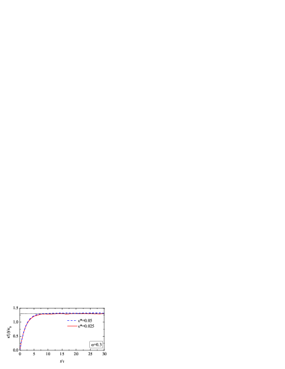
Figure 1: (Color online) Plot of the time-dependent (modified) thermal conductivity versus time for $\alpha=0.3$ and $\epsilon^{*}=0.05$ (dashed line) and $\epsilon^{*}=0.025$ (solid line). The horizontal dotted line indicates the steady-state value averaged over time in the case $\epsilon^{*}=0.025$.

An additional test of the linear regime is provided by Fig. 2, which shows the time evolution of the Sonine coefficients $b_{1}^{\prime}$, $b_{2}^{\prime}$, and $b_{3}^{\prime}$ for $\alpha=1$ and $\alpha=0.3$. These coefficients have been evaluated from Eq. (57) and also from Eq. (59). As proven in the Appendix, both methods must lead to identical results, provided that the system is in the linear regime. Figure 2 shows that the simulation data obtained from $\langle c_{x}L_{k}^{(3/2)}(c^{2})\rangle$ are practically indistinguishable from those obtained from $\langle c_{x}L_{k}^{(1/2)}(c_{x}^{2})\rangle$, thus confirming that the value $\epsilon^{*}=0.025$ is small enough to assume that the system is actually in the linear regime. Given that the fluctuations are smaller when the Sonine coefficients are computed from $\langle c_{x}L_{k}^{(3/2)}(c^{2})\rangle$ than when they are computed from $\langle c_{x}L_{k}^{(1/2)}(c_{x}^{2})\rangle$, henceforth we choose the former method. We also see in Fig. 2 that the characteristic relaxation time ($t/\tau\sim 10$) is practically independent of the degree of inelasticity as well as of the order of the Sonine coefficient considered.

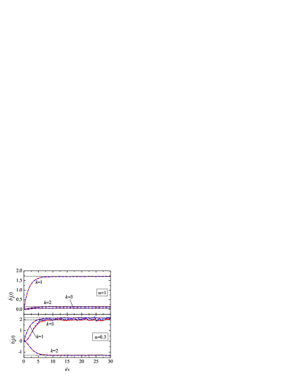
Figure 2: (Color online) Plot of the time-dependent Sonine coefficients $b_{k}^{\prime}$ ($k=1,2,3$) versus time for $\alpha=1$ (top panel) and $\alpha=0.3$ (bottom panel). The solid and dahed lines correspond to data obtained from $\langle c_{x}L_{k}^{(3/2)}(c^{2})\rangle$ and from $\langle c_{x}L_{k}^{(1/2)}(c_{x}^{2})\rangle$, respectively. Note that they are distinguishable only in the case of $b_{3}^{\prime}$ for $\alpha=0.3$. The horizontal dotted lines indicate the steady-state values.

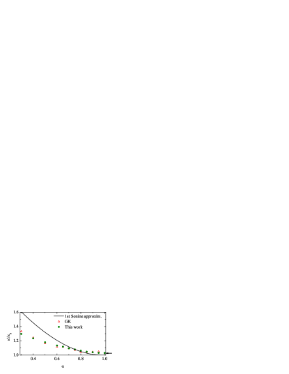
Figure 3: (Color online) Plot of the modified thermal conductivity coefficient $\kappa^{\prime}$ versus the coefficient of normal restitution $\alpha$. The circles refer to the simulation data obtained by the method described in this paper, while the triangles refer to the simulation data obtained in Ref. BRMMG05 from the GK relations. We have checked that the error bars of our simulation data are smaller than the size of the symbols. The solid line is the prediction given by the first Sonine approximation. The arrow indicates the value $\kappa/\kappa_{0}=1.025218$ corresponding to the elastic limit when higher order terms in the Sonine expansion are taken into account.

Now we focus on the dependence of the steady-state quantities on dissipation. Figure 3 shows $\kappa^{\prime}/\kappa_{0}$ as a function of the coefficient of restitution $\alpha$. In addition to our simulation data, we have included the values of $\kappa^{\prime}$ obtained from the simulation data of $\kappa$ and $\mu$ reported by Brey et al. BRMMG05 , as well as the first Sonine approximation given by Eqs. (42) and (46). It must be emphasized that the methods used here and in Ref. BRMMG05 are quite different. In the latter method, two-time correlation functions of certain quantities are evaluated in the HCS and subsequently those correlation functions are integrated in time to get the transport coefficients. On the other hand, in our method the HCS is slightly perturbed by a homogeneous external forcing and the transport coefficient is determined from a standard one-time average (namely, the heat flux), by assuming linear response. While the first Sonine prediction does a good job for $\alpha\gtrsim 0.7$, it dramatically overestimates the thermal conductivity for higher inelasticity. It is important to remark that the excellent agreement found between both simulation methods strongly supports the conclusion that the discrepancies between the first Sonine approximation and simulations are not due to the presence of velocity correlations beyond the Boltzmann description for strong dissipation. Instead, those discrepancies are essentially due to the inaccuracy of the first Sonine approximation for $\alpha\lesssim 0.7$. In the elastic limit, the numerical results show that the first Sonine approximation slightly underestimates the thermal conductivity. This is known to be corrected if higher orders in the Sonine polynomial expansion are taken into account CC70 , which yields $\kappa/\kappa_{0}=1.025218$ Gallis . This value is indicated by an arrow in Fig. 3 and agrees with our simulation result for $\alpha=1$.

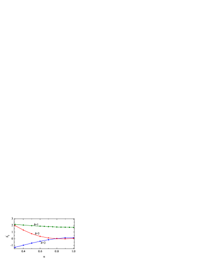
Figure 4: (Color online) Plot of the Sonine coefficients $b_{1}^{\prime}$ (circles), $b_{2}^{\prime}$ (squares), and $b_{3}^{\prime}$ (triangles) versus the coefficient of normal restitution $\alpha$. The error bars are smaller than the size of the symbols. The lines are guides to the eye.

The above conclusion about the strong inaccuracy of the first Sonine approximation for $\alpha\lesssim 0.7$ is further confirmed by Fig. 4, which shows the $\alpha$-dependence of the three first Sonine coefficients. We observe that $b_{1}^{\prime}$ is much less sensitive to dissipation than $b_{2}^{\prime}$ and $b_{3}^{\prime}$. For not too large inelasticity ($\alpha\gtrsim 0.7$), the second and third Sonine coefficients are much smaller than $b_{1}^{\prime}$ and, consequently, one may expect that the series (44) truncated after $k=1$ is sufficiently close to the true distribution $\bm{\mathcal{A}}^{\prime}$, at least in the region of thermal velocities relevant for the evaluation of the heat flux. On the other hand, as dissipation increases beyond $\alpha\approx 0.7$, the magnitude of the coefficients $b_{2}^{\prime}$ and $b_{3}^{\prime}$ grow rapidly, becoming comparable to $b_{1}^{\prime}$. This implies that contributions to $\bm{\mathcal{A}}^{\prime}$ beyond the first Sonine term cannot be neglected. In principle, the discrepancies of the first Sonine approximation could be remedied by considering the second Sonine approximation, i.e., by truncating the expansion (44) after $k=2$. However, according to Fig. 4, there does not exist a range of values of $\alpha$ where the magnitude of $b_{3}^{\prime}$ is much smaller than that of $b_{2}^{\prime}$, so that the second Sonine approximation possibly would not be sufficient.

It is worthwhile remarking that the characteristic value of $\alpha$ approximately below which the first Sonine approximation begins to deviate significantly from the simulation data is also the value below which the fourth cumulant $a_{2}$ of the HCS starts to grow MS00 ; CDPT03 ; BCRM99 ; BP06 . This means that there seems to be a close relationship between the deviation of the HCS distribution $f^{(0)}$ from its Gaussian form and the deviation of the NS distribution $f^{(1)}$ from its first Sonine approximation. Given that the weight function in the Sonine expansion is the Gaussian, it seems natural to conjecture that a better estimate of $f^{(1)}$ can be obtained by replacing the Gaussian weight function by the HCS distribution $f^{(0)}$ L05 ; GS06 .

One of the advantages of the simulation method devised in this paper is that it allows to measure not only the transport coefficient $\kappa^{\prime}$ or higher velocity moments (such as those associated with $b_{2}^{\prime}$ and $b_{3}^{\prime}$), but also the NS velocity distribution function itself. As said in Sec. III, all the information contained in the full distribution $f^{(1)}(\mathbf{V})$ is present in the marginal distribution function $g^{(1)}({V}_{x})$ defined by Eq. (60). Thus, in what follows, we restrict ourselves to this marginal distribution function, which can be computed more efficiently than $f^{(1)}(\mathbf{V})$ in the simulations. In order to analyze $g^{(1)}({V}_{x})$, it is convenient to write it in the form

$$g^{(1)}({V}_{x})=nv_{0}^{-1}\pi^{-1/2}e^{-c_{x}^{2}}c_{x}\varphi(c_{x}^{2})\epsilon^{*},$$ (71)

where $\varphi(c_{x}^{2})$ is a dimensionless isotropic function, independent of $\epsilon^{*}$. Its Sonine expansion is

$$\varphi(c_{x}^{2})=\sum_{k=1}^{\infty}b_{k}^{\prime}L_{k}^{(1/2)}(c_{x}^{2}),$$ (72)

where, as proven in the Appendix, the coefficients $b_{k}^{\prime}$ are the same as in the Sonine expansion (44). For the sake of comparison, it is convenient to introduce the truncated series

$$\varphi_{p}(c_{x}^{2})=\sum_{k=1}^{p}b_{k}^{\prime}L_{k}^{(1/2)}(c_{x}^{2}).$$ (73)

If the first Sonine approximation is reliable, this means that $\varphi(c_{x}^{2})\simeq\varphi_{1}(c_{x}^{2})\equiv b_{1}^{\prime}(\frac{3}{2}-c_{x}^{2})$ in the region of thermal velocities (say $c_{x}^{2}\lesssim 10$). In addition, one would expect that an even better approximation would be obtained with $\varphi_{2}(c_{x}^{2})$ and $\varphi_{3}(c_{x}^{2})$.

The function $\varphi(c_{x}^{2})$ is plotted in Figs. 5 (for $\alpha=1$ and $\alpha=0.9$) and 6 (for $\alpha=0.7$, $\alpha=0.5$, and $\alpha=0.3$). The first three truncated polynomials $\varphi_{p}(c_{x}^{2})$, $p=1,2,3$, obtained by using the simulation values of $b_{p}^{\prime}$, are also plotted. In Fig. 5 we observe that the first Sonine polynomial $\varphi_{1}(c_{x}^{2})$ captures reasonably well the behavior of the true distribution $\varphi(c_{x}^{2})$, although it underestimates the latter for $c_{x}^{2}\gtrsim 4$. The addition of the second and third Sonine polynomials significantly improves the agreement with the true distribution. In fact, $\varphi_{3}$ is practically indistinguishable from $\varphi$.

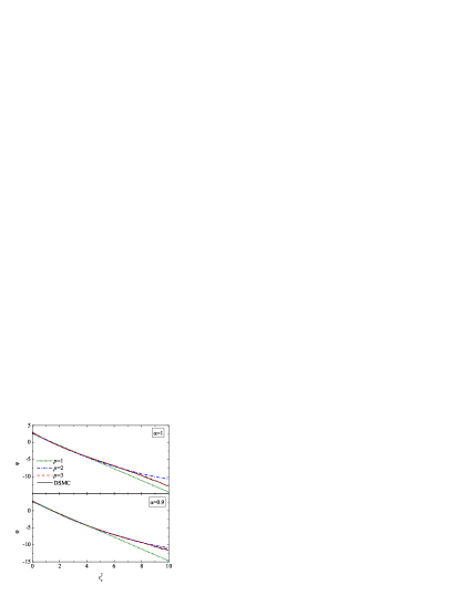
Figure 5: (Color online) Plot of the distribution function $\varphi(c_{x}^{2})$ (solid lines) for $\alpha=1$ (top panel) and $\alpha=0.9$ (bottom panel). The dotted, dotted-dashed, and dashed lines correspond to the truncated Sonine expansions $\varphi_{p}(c_{x}^{2})$ with $p=1$, 2, and 3, respectively.

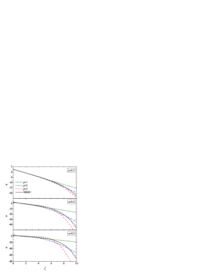
Figure 6: (Color online) Plot of the distribution function $\varphi(c_{x}^{2})$ (solid lines) for $\alpha=0.7$ (top panel), $\alpha=0.5$ (middle panel), and $\alpha=0.3$ (bottom panel). The dotted, dotted-dashed, and dashed lines correspond to the truncated Sonine expansions $\varphi_{p}(c_{x}^{2})$ with $p=1$, 2, and 3, respectively.

As the inelasticity increases, so does the deviation of $\varphi$ from the first Sonine polynomial, as shown in Fig. 6. In contrast to the situation in Fig. 5, $\varphi_{1}$ overestimates the function $\varphi$ for large velocities. Moreover, the second and third Sonine truncated expansions do not clearly improve the agreement, especially for $\alpha=0.5$ and $\alpha=0.3$.

The comparison carried out in Figs. 5 and 6 confirms that, if $\alpha\lesssim 0.7$, the velocity distribution function is not sufficiently well described by the first term in the Sonine expansion and, consequently, the value of $b_{1}^{\prime}$ (and hence of $\kappa^{\prime}$) estimated from the first Sonine approximation is not accurate. It is also interesting to note that when $\varphi_{1}$ underestimates (overestimates) the function $\varphi$ for large velocities, $\kappa^{\prime}$ tends to be underestimated (overestimated) by the first Sonine approximation. In view of the panels corresponding to $\alpha=0.5$ and $\alpha=0.3$ in Fig. 6, it is highly questionable that the second or third Sonine approximations could provide accurate estimates for $\kappa^{\prime}$. An alternative route has been recently proposed GS06 .

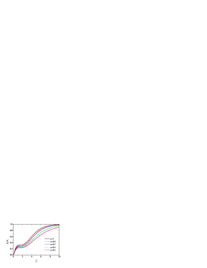
Figure 7: (Color online) Plot of the ratio $\beta_{1}(c_{x}^{2})/b_{1}^{\prime}$ for $\alpha=1$, 0.9, 0.7, 0.5, and 0.3.

Finally, we address the question on the velocity range relevant to the evaluation of $\kappa^{\prime}\propto b_{1}^{\prime}$. According to Figs. 5 and 6, if that range were, for instance, $0\leq c_{x}^{2}\lesssim 6$, then the first Sonine estimate would be reliable even for $\alpha=0.3$. Since this is not the case, it is obvious that the population of particles with $c_{x}^{2}\gtrsim 6$ must have a significant influence on the heat flux for large inelasticity. To analyze this point with more detail, let us introduce the function

$$\beta_{1}(c_{x}^{2})=\frac{8}{3\pi^{1/2}}\int_{0}^{c_{x}^{2}}du_{x}\,u_{x}^{2}\left(\frac{3}{2}-u_{x}^{2}\right)e^{-u_{x}^{2}}\varphi(u_{x}^{2}).$$ (74)

This function represents the contribution to $b_{1}^{\prime}$ coming from particles whose $x$-component of the (reduced) velocity is smaller than $|c_{x}|$, so that $\lim_{c_{x}^{2}\to\infty}\beta_{1}(c_{x}^{2})=b_{1}^{\prime}$. The ratio $\beta_{1}(c_{x}^{2})/b_{1}^{\prime}$ is plotted in Fig. 7 for the same values of $\alpha$ as in Figs. 5 and 6. We see that the larger the inelasticity, the wider the range of velocities needed to faithfully evaluate $b_{1}^{\prime}$. For instance, particles with $0\leq c_{x}^{2}\leq 6$ contribute to 87% of the heat flux in the elastic case, while that percentage reduces to 66% in the case of $\alpha=0.3$.

V Conclusions

The CE solution of the inelastic Boltzmann equation provides expressions for the NS transport coefficients in terms of the solutions of linear integral equations BDKS98 . Alternatively, these expressions can be proven to be equivalent to GK relations DB02 . In either case, in order to obtain the explicit dependence of the transport coefficients on the coefficient of restitution, one needs to make use of certain approximations. As in the case of elastic collisions, the standard approach is to expand the unknown NS velocity distribution function in Sonine polynomials and truncate it at a given order. Of course, the practical difficulties increase considerably with the number of retained polynomials, so the first Sonine approximation is usually chosen. To check the reliability of the first Sonine approximation one needs to resort to comparison with DSMC computer simulations of the Boltzmann equation. In principle, there are two strategies to measure the transport coefficients via computer simulations in homogeneous states. One consists of measuring the appropriate time correlation functions in the HCS and then carry out an integration over time by applying the GK relations DB02 . In the other possible strategy, one weakly disturbs the granular gas from the HCS by the action of a conveniently chosen homogeneous, anisotropic external force that produces the same effect as a hydrodynamic gradient; in this way, the simulations provide in the linear response regime the transport coefficients as well as the NS velocity distribution functions. The first method has been used to get the shear viscosity $\eta$ and the two transport coefficients ($\kappa$ and $\mu$) associated with the heat flux BRM04 ; BRMMG05 , while so far the second method has only been applied to $\eta$ MSG05 .

The first Sonine approximation for $\eta$ is seen to compare quite well with DSMC simulations, even for strong dissipation BRM04 ; BRMMG05 ; MSG05 . However, the corresponding approximations for $\kappa$ and $\mu$ appreciably differ from GK simulations for high inelasticity ($\alpha\lesssim 0.7$). One could argue that these discrepancies are a reflection of the velocity correlations appearing in the HCS, even in the low-density limit. In that scenario, the correlation functions computed in DSMC simulations would incorporate effects not accounted for by the Boltzmann equation.

The primary goal of this paper has been to investigate whether the discrepancies observed between the first Sonine estimates and the GK data are due to effects beyond the Boltzmann framework or are simply due to the limitations of the first Sonine approach. To that end, we have followed the second strategy mentioned above, namely, the one based on the action of a homogeneous external force. First, we have derived the explicit forms of the respective velocity-dependent external forces which yield, to first order, the NS velocity distribution functions associated with the standard thermal conductivity $\kappa$ and the modified thermal conductivity $\kappa^{\prime}\equiv\kappa-n\mu/2T$. In the case of $\kappa$, the external force must be complemented by a stochastic term describing a clonation-annihilation process. Since the presence of this latter term complicates the simulation method, in this paper we have focused on the homogeneous Boltzmann equation corresponding to the coefficient $\kappa^{\prime}$. Our DSMC results show an excellent consistency with those obtained in Ref. BRMMG05 by the GK formalism. Since our method is entirely tied to the Boltzmann equation, we conclude that the deviations of the simulation data from the first Sonine approximation are mainly due to the inaccuracy of the latter. This conclusion has been further supported by an analysis of the first three Sonine coefficients and of the NS velocity distribution function itself. While the second and third Sonine coefficients are practically negligible for $\alpha\gtrsim 0.7$, they rapidly increase in magnitude as the inelasticity increases, becoming comparable to the first Sonine coefficient. With respect to the distribution function, we have observed that, for strong dissipation, it is not well captured by the first Sonine polynomial in the whole velocity region relevant to the computation of the transport coefficient $\kappa^{\prime}$.

The simulation results reported in this paper indicate that the second or third Sonine approximations are not expected to improve significantly the quality of the first Sonine estimate, especially considering the technical difficulties associated with the method. An alternative avenue under the form of a modified first Sonine approximation is explored elsewhere GS06 .

*

Appendix A Proof of the equivalence between Eqs. (57) and (59)

The full NS velocity distribution function (55) can be written as

$$f^{(1)}(\mathbf{V})=nv_{0}^{-d}\pi^{-d/2}e^{-c^{2}}c_{x}\Phi(c^{2})\epsilon^{*},$$ (75)

where $\Phi(c^{2})$ is a dimensionless isotropic function. This function can be expanded in Laguerre (or Sonine) polynomials as

$$\Phi(c^{2})=\sum_{k=1}^{\infty}b_{k}^{\prime}L_{k}^{(d/2)}(c^{2}),$$ (76)

in agreement with Eq. (44). The orthogonality condition (12) yields

$$b_{k}^{\prime}=\frac{2\Gamma(1+d/2)k!}{\Gamma(k+1+d/2)}\pi^{-d/2}\int d\mathbf{c}\,c_{x}^{2}e^{-c^{2}}L_{k}^{(d/2)}(c^{2})\Phi(c^{2}).$$ (77)

This expression is equivalent to Eq. (57).

Let us now consider the marginal distribution $g^{(1)}(V_{x})$ defined by Eq. (60). Similarly to Eq. (75), $g^{(1)}(V_{x})$ can be expressed as Eq. (71). Thus, the function $\varphi(c_{x}^{2})$ can be obtained from $\Phi(c^{2})$ as

$$\varphi(c_{x}^{2})=\pi^{-(d-1)/2}\int d\mathbf{c}_{\perp}\,e^{-c_{\perp}^{2}}\Phi(c^{2}).$$ (78)

Inserting the expansion (76) we get

$$\varphi(c_{x})=\sum_{k=1}^{\infty}b_{k}^{\prime}F_{k}(c_{x}^{2}),$$ (79)

where we have called

$$F_{k}(c_{x}^{2})\equiv\pi^{-(d-1)/2}\int d\mathbf{c}_{\perp}\,e^{-c^{2}_{\perp}}L_{k}^{(d/2)}(c^{2}).$$ (80)

Now we make use of the mathematical property AS72

$$L_{k}^{(p+q+1)}(x+y)=\sum_{\ell=0}^{k}L_{\ell}^{(p)}(x)L_{k-\ell}^{(q)}(y)$$ (81)

and take $p=1/2$, $q=(d-3)/2$, $x=c_{x}^{2}$, and $y=c_{\perp}^{2}$. Thus,

$$F_{k}(c_{x}^{2})=\pi^{-(d-1)/2}\sum_{\ell=0}^{k}L_{\ell}^{(1/2)}(c_{x}^{2})\int d\mathbf{c}_{\perp}\,e^{-c^{2}_{\perp}}L_{k-\ell}^{(\frac{d-3}{2})}(c_{\perp}^{2}).$$ (82)

The integral can be computed as

$$\pi^{-(d-1)/2}\int d\mathbf{c}_{\perp}\,e^{-c^{2}_{\perp}}L_{k-\ell}^{(\frac{d-3}{2})}(c_{\perp}^{2})$$

$$=\frac{1}{\Gamma((d-1)/2)}\int_{0}^{\infty}dy\,y^{(d-3)/2}L_{k-\ell}^{(\frac{d-3}{2})}(y)$$

$$=\delta_{k,\ell},$$ (83)

where in the last step we have made use of the orthogonality relation of the generalized Laguerre polynomials. Therefore, $F_{k}(c_{x}^{2})=L_{k}^{(1/2)}(c_{x}^{2})$ and so Eq. (79) becomes

$$\varphi(c_{x}^{2})=\sum_{k=1}^{\infty}b_{k}^{\prime}L_{k}^{(1/2)}(c_{x}^{2}).$$ (84)

From here one can obtain an alternative expression for the coefficients $b_{k}^{\prime}$ as

$$b_{k}^{\prime}=\frac{2\Gamma(3/2)k!}{\Gamma(k+3/2)}\pi^{-1/2}\int_{-\infty}^{\infty}d{c}_{x}\,c_{x}^{2}e^{-c_{x}^{2}}L_{k}^{(1/2)}(c_{x}^{2})\varphi(c_{x}^{2}).$$ (85)

This is equivalent to Eq. (59).

References

- (1) C. S. Campbell, Annu. Rev. Fluid Mech. 22 (1990) 57; I. Goldhirsch, ibid. 35 (2003) 267.
- (2) I. Goldhirsch and T. P. C. van Noije, Phys. Rev. E 61 (2000) 3241.
- (3) J. W. Dufty and V. Garzó, J. Stat. Phys. 105 (2001) 723.
- (4) J. W. Dufty, J. J. Brey, and J. Lutsko, Phys. Rev. E 65 (2002) 051303.
- (5) J. W. Dufty and J. J. Brey, J. Stat. Phys. 109 (2002) 433.
- (6) J. J. Brey, J. W. Dufty, and M. J. Ruiz-Montero, in Granular Gas Dynamics, edited by T. Pöschel and N. Brilliantov, Springer, Berlin, 2003, pp. 227–249.
- (7) J. Dufty, A. Baskaran, and J. J. Brey, J. Stat. Mech. (2006) L08002.
- (8) A. Goldshtein and M. Shapiro, J. Fluid Mech. 282 (1995) 75.
- (9) J. J. Brey, J. W. Dufty, and A. Santos, J. Stat. Phys. 87 (1997) 1051.
- (10) J. J. Brey and M. J. Ruiz-Montero, Phys. Rev. E 70 (2004) 051301.
- (11) J. J. Brey, M. J. Ruiz-Montero, P. Maynar, and M. I. García de Soria, J. Phys.: Condens. Matter 17 (2005) S2489.
- (12) S. Chapman and T. G. Cowling, The Mathematical Theory of Nonuniform Gases, Cambridge University Press, Cambridge, 1970.
- (13) J. J. Brey, J. W. Dufty, C. S. Kim, and A. Santos, Phys. Rev. E 58 (1998) 4638.
- (14) J. J. Brey and D. Cubero, in Granular Gases, edited by T. Pöschel and S. Luding, Springer-Verlag, Berlin, 2001, pp. 59–78.
- (15) V. Garzó and J. M. Montanero, Physica A 313 (2002) 336.
- (16) V. Garzó and J. W. Dufty, Phys. Fluids 14 (2002) 1476; V. Garzó and J. M. Montanero, Phys. Rev. E 69 (2004) 021301.
- (17) V. Garzó and J. W. Dufty, Phys. Rev. E 59 (1999) 5895.
- (18) J. F. Lutsko, Phys. Rev. E 72 (2005) 021306.
- (19) J. J. Brey, M. J. Ruiz-Montero, and D. Cubero, Europhys. Lett. 48 (1999) 359.
- (20) J. M. Montanero and V. Garzó, Phys. Rev. E 67 (2003) 021308; V. Garzó and J. M. Montanero, ibid. 68 (2003) 041302.
- (21) J. M. Montanero, A. Santos, and V. Garzó, in Rarefied Gas Dynamics: 24th International Symposium on Rarefied Gas Dynamics, edited by M. Capitelli, AIP Conference Proceedings, vol. 762, Melville, NY, 2005, pp. 797–802; preprint cond-mat/0411219.
- (22) D. J. Evans, Phys. Lett. A 91, 457 (1982).
- (23) M. J. Gillan and M. Dixon, J. Phys. C: Solid State Phys. 16 (1983) 869.
- (24) D. J. Evans, Phys. Rev. A 34 (1986) 1449.
- (25) J. M. Montanero and A. Santos, in Rarefied Gas Dynamics 20, edited by C. Shen, Peking University Press, Beijing, 1997) pp. 137–142.
- (26) W. Loose, Phys. Rev. A 40 (1989) 2625.
- (27) V. Garzó and A. Santos, Chem. Phys. Lett. 177 (1991) 79.
- (28) V. Garzó, A. Santos, and J. M. Montanero, Modified Sonine approximation for the Navier–Stokes transport coefficients of a granular gas, preprint cond-mat/0604079.
- (29) T. P. C. van Noije and M. H. Ernst, Gran. Matt. 1 (1998) 57.
- (30) S. E. Esipov and T. Pöschel, J. Stat. Phys. 86 (1997) 1385.
- (31) Handbook of Mathematical Functions, edited by M. Abramowitz and I. A. Stegun, Dover, New York, 1972.
- (32) J. M. Montanero and A. Santos, Gran. Matt. 2 (2000) 53.
- (33) F. Coppex, M. Droz, J. Piasecki, and E. Trizac, Physica A 329 (2003) 114.
- (34) J. J. Brey and J. W. Dufty, Phys. Rev. E 72 (2005) 011303.
- (35) G. Bird, Molecular Gas Dynamics and the Direct Simulation of Gas Flows, Clarendon, Oxford, 1994) F. J. Alexander and A. L. Garcia, Comp. Phys. 11 (1997) 588.
- (36) W. Wagner, J. Stat. Phys. 66 (1992) 1011.
- (37) M. A. Gallis, J. R. Torczynski, and D. J. Rader, Phys. Rev. E 69 (2004) 042201.
- (38) J. J. Brey, D. Cubero, and M. J. Ruiz-Montero, Phys. Rev. E 59 (1999) 1256.
- (39) N. V. Brilliantov and Pöschel, Europhys. Lett. 74 (2006) 424; Erratum: 75 (2006) 188.