Modified Sonine approximation for the Navier–Stokes transport coefficients of a granular gas

Abstract

Motivated by the disagreement found at high dissipation between simulation data for the heat flux transport coefficients and the expressions derived from the Boltzmann equation by the standard first Sonine approximation [Brey et al., Phys. Rev. E 70, 051301 (2004); J. Phys.: Condens. Matter 17, S2489 (2005)], we implement in this paper a modified version of the first Sonine approximation in which the Maxwell–Boltzmann weight function is replaced by the homogeneous cooling state distribution. The structure of the transport coefficients is common in both approximations, the distinction appearing in the coefficient of the fourth cumulant $a_{2}$. Comparison with computer simulations shows that the modified approximation significantly improves the estimates for the heat flux transport coefficients at strong dissipation. In addition, the slight discrepancies between simulation and the standard first Sonine estimates for the shear viscosity and the self-diffusion coefficient are also partially corrected by the modified approximation. Finally, the extension of the modified first Sonine approximation to the transport coefficients of the Enskog kinetic theory is presented.

Keywords: Granular gases; Boltzmann kinetic theory; Navier–Stokes transport coefficients; Sonine approximation

I Introduction

The usefulness of kinetic theory tools to describe the dynamical properties of granular fluids has been widely recognized C90 ; BP04 . The primary difference from normal fluids lies in the inelastic character of collisions, what introduces features not present in ordinary matter, such as the absence of equilibrium states, the spontaneous formation of clusters, and the development of high-energy tails, among others. The prototype model of a granular gas is a system composed by a large number of smooth hard spheres colliding inelastically with a constant coefficient of normal restitution $0<\alpha\leq 1$. In the dilute limit, the Boltzmann kinetic equation, suitably modified to incorporate inelasticity, provides a convenient framework to investigate some of the most relevant properties of granular gases.

One of the main applications of the inelastic Boltzmann equation is the derivation of the constitutive equations for the stress tensor and the heat flux in a hydrodynamic description. These constitutive equations define the relevant Navier–Stokes (NS) transport coefficients and are determined by means of the Chapman–Enskog (CE) method to solve the Boltzmann equation for sufficiently long space and time scales. While in the elastic case the velocity distribution function $f$ is expanded about the local equilibrium distribution function $f_{M}$, the reference state for granular gases is the local version $f^{(0)}$ of the so-called homogeneous cooling state (HCS). The first-order stage of the CE expansion allows one to express the transport coefficients in terms of the solutions of linear integral equations BDKS98 ; GD99 ; BC01 ; GD02 ; L05 . In these equations the distribution $f^{(0)}$ appears explicitly in the inhomogeneous terms and implicitly through the linearized Boltzmann collision operator. As happens in the elastic case, the solutions of the integral equations are not known exactly, so that approximations must be introduced in order to get the transport coefficients as explicit nonlinear functions of $\alpha$. The standard method consists of approximating the solutions by the Maxwell–Boltzmann distribution $f_{M}$ times truncated Sonine polynomial expansions. The simplest possibility is the first Sonine approximation, where only the lowest Sonine polynomial is retained. The resulting expressions for the effective collision frequencies associated with the transport coefficients have an explicit dependence on $\alpha$ (due to the collision rules) as well as an implicit one through a linear dependence on the fourth cumulant $a_{2}$ of $f^{(0)}$.

The reliability of the standard first Sonine approximation has been tested in the last few years BRMC99 ; BRMCGR00 ; LBD02 ; GM02 ; MG03 ; GM04 ; BRM04 ; BRMMG05 ; MSG05 ; MSG06 by comparison with computer simulations of the Boltzmann equation by means of the direct simulation Monte Carlo (DSMC) method DSMC . The comparisons show that the shear viscosity $\eta$ and the self-diffusion coefficient $D$ are accurately estimated by the first Sonine approximation, even for strong dissipation. The two transport coefficients $\kappa$ and $\mu$ characterizing the heat flux are well described by the first Sonine approximation for moderate and small inelasticity (say $\alpha\gtrsim 0.7$). However, recent studies BRM04 ; BRMMG05 show that the first Sonine approximation dramatically overestimates $\kappa$ and $\mu$ for high dissipation ($\alpha\lesssim 0.7$).

Although the range $\alpha\gtrsim 0.7$ encompasses the region of practical and experimental interest, especially if one considers the inherent coupling between gradients and dissipation in steady states BC98 ; SGD04 , it is important from a fundamental point of view to understand the origin of those discrepancies for $\kappa$ and $\mu$ and propose alternative approximations. Since in the simulations carried out in Refs. BRM04 ; BRMMG05 the transport coefficients were obtained from two-time correlation functions by means of Green–Kubo (GK) relations, the discrepancies might be due to velocity correlation effects outside the domain of the Boltzmann equation. However, as discussed in Ref. MSG06 , the disagreement seems to be directly related to the failure of the Sonine expansion truncated after the first term to capture the velocity dependence of the NS distribution function. One possibility of improving the approximation could be to consider higher order terms in the Sonine expansion GM04 . However, the involved algebra would be rather intricate and it is not obvious that the improvement would be significant.

The aim of this paper is to implement an alternative route to the standard first Sonine approximation. The idea is based on the assumption that the isotropic part of the NS velocity distribution $f^{(1)}$ is mainly governed by the HCS distribution $f^{(0)}$ rather than by the Maxwellian distribution $f_{M}$ L05 . More specifically, our modified first Sonine approximation has the same form as the standard one, except that the weight function $f_{M}$ is replaced by $f^{(0)}$. As a consequence, the effective collision frequencies derived from the modified approximation have the same structure as those derived from the standard one, except that the respective coefficients of $a_{2}$ differ markedly in both approximations. Since the high-velocity population in $f^{(0)}$ is larger than in $f_{M}$, it is reasonably expected that the former captures better the influence of the high-velocity tail of $f^{(1)}$ on the NS transport coefficients, especially those related to the heat flux. In fact, the results show that, in the region $\alpha\lesssim 0.7$, the modified values for the collision frequencies are larger than their standard counterparts, so that the corresponding transport coefficients are smaller in the modified first Sonine approximation than in the standard one. As will be shown later, the modified estimates for the transport coefficients $\kappa$ and $\mu$ compare quite well with available computer simulations, even for extreme dissipation, in contrast to what happens with the standard estimates. For the remaining transport coefficients $\eta$ and $D$, which are already well described by the standard approximation, the modified approximation provides even better values.

The plan of the paper is as follows. The expressions of the NS transport coefficients obtained by the application of the standard first Sonine approximation are recalled in Sec. II. Our modified first Sonine approximation is described and discussed in Sec. III. Next, the two Sonine approximations are compared in Sec IV with available and new simulation data for the transport coefficients $\kappa$, $\mu$, $\eta$, and $D$, both for two- and three- dimensional systems. The extension to the transport coefficients provided by the Enskog theory is presented in Appendix B. The paper is closed with some concluding remarks in Sec. V.

II Standard first Sonine approximation

We consider a granular gas of smooth, inelastic hard spheres (in $d$ dimensions) of mass $m$, diameter $\sigma$, and coefficient of restitution $\alpha$. In the low-density regime, the one-particle velocity distribution function $f({\bf r},{\bf v},t)$ obeys the (inelastic) Boltzmann equation GS95 ; BDS97 . Under the conditions of weak hydrodynamic gradients, the CE method CC70 provides a solution of the Boltzmann equation based on an expansion $f=f^{(0)}+f^{(1)}+\cdots$, where $f^{(0)}$ is the local version of the HCS GS95 ; vNE98 . The first-order distribution $f^{(1)}$ has the form BDKS98 ; BC01

$$f^{(1)}({\bf V})={\bm{\mathcal{A}}}({\bf V})\cdot\nabla\ln T+{\bm{\mathcal{B}}}({\bf V})\cdot\nabla\ln n+{\cal C}_{ij}({\bf V})\nabla_{i}u_{j},$$ (1)

where $n$, $T$, and $\mathbf{u}$ are the number density, granular temperature, and flow velocity, respectively, and $\mathbf{V}=\mathbf{v}-\mathbf{u}$ is the peculiar velocity. The functions ${\bm{\mathcal{A}}}({\bf V})$, ${\bm{\mathcal{B}}}({\bf V})$, and ${\cal C}_{ij}({\bf V})$ are the solutions of a set of linear integral equations. While ${\bm{\mathcal{A}}}({\bf V})$ and ${\cal C}_{ij}({\bf V})$ obey autonomous equations, the equation for ${\bm{\mathcal{B}}}({\bf V})$ requires the knowledge of ${\bm{\mathcal{A}}}({\bf V})$. However, the combination ${\bm{\mathcal{A}}}^{\prime}({\bf V})={\bm{\mathcal{A}}}({\bf V})-\frac{1}{2}{\bm{\mathcal{B}}}({\bf V})$ satisfies a closed equation MSG06 . From the solutions to those linear integral equations, the shear viscosity $\eta$ (associated with the pressure tensor), the thermal conductivity $\kappa$, and a new transport coefficient $\mu$ (the two latter associated with the heat-flux) are formally given by BDKS98 ; BC01 ; MSG06

$$\eta=\eta_{0}\frac{1}{\nu_{\eta}^{*}-\frac{1}{2}\zeta^{*}},$$ (2)

$$\kappa=\kappa_{0}\frac{d-1}{d}\frac{1+2a_{2}}{\nu_{\kappa}^{*}-2\zeta^{*}},$$ (3)

$$\mu=\frac{2T}{n}(\kappa-\kappa^{\prime}),\quad\kappa^{\prime}=\kappa_{0}\frac{d-1}{d}\frac{1+\frac{3}{2}a_{2}}{\nu_{\kappa^{\prime}}^{*}-\frac{3}{2}\zeta^{*}},$$ (4)

where, $\eta_{0}$ and $\kappa_{0}$ are the elastic values (in the first Sonine approximation) of the shear viscosity and thermal conductivity CC70 , respectively [cf. Eq. (57)]. In addition, $\zeta^{*}=\zeta^{(0)}/\nu_{0}$ is the reduced cooling rate of the HCS, where $\nu_{0}=nT/\eta_{0}$ is an effective collision frequency [cf. Eq. (59)], and $a_{2}$ is the fourth velocity cumulant of $f^{(0)}$. Furthermore, in Eqs. (2)–(4) the (reduced) effective collision frequencies are

$$\nu_{\eta}^{*}=\frac{\int d{\bf v}D_{ij}({\bf V}){\cal L}{\cal C}_{ij}({\bf V})}{\nu_{0}\int d{\bf v}D_{ij}({\bf V}){\cal C}_{ij}({\bf V})},$$ (5)

$$\nu_{\kappa}^{*}=\frac{\int d{\bf v}{\bf S}({\bf V})\cdot{\cal L}{\bm{\mathcal{A}}}({\bf V})}{\nu_{0}\int d{\bf v}{\bf S}({\bf V})\cdot{\bm{\mathcal{A}}}({\bf V})},\quad\nu_{\kappa^{\prime}}^{*}=\frac{\int d{\bf v}{\bf S}({\bf V})\cdot{\cal L}{\bm{\mathcal{A}}}^{\prime}({\bf V})}{\nu_{0}\int d{\bf v}{\bf S}({\bf V})\cdot{\bm{\mathcal{A}}}^{\prime}({\bf V})},$$ (6)

where ${\cal L}$ is the linearized Boltzmann collision operator and we have introduced the polynomials

$$D_{ij}(\mathbf{V})=m\left({V}_{i}{V}_{j}-\frac{1}{d}V^{2}\delta_{ij}\right),$$ (7)

$$\mathbf{S}(\mathbf{V})=\left(\frac{m}{2}V^{2}-\frac{d+2}{2}T\right){\bf V}.$$ (8)

Another relevant transport coefficient for a single gas is the self-diffusion coefficient $D$, which measures the diffusion of tagged particles in a fluid of mechanically equivalent particles in the HCS. Application of the CE method leads to $f_{s}^{(0)}=(n_{s}/n)f^{(0)}$ and

$$f^{(1)}_{s}(\mathbf{V})=\bm{\mathcal{D}}(\mathbf{V})\cdot\nabla n_{s},$$ (9)

where $n_{s}$ and $f_{s}$ are the number density and velocity distribution function of the tagged particles, respectively. As before, the function $\bm{\mathcal{D}}(\mathbf{V})$ is the solution of a linear integral equation. The CE expression for the self-diffusion coefficient $D$ is BRMCGR00 ; GM04

$$D=D_{0}\frac{d+2}{2d}\frac{1}{\nu_{D}^{*}-\frac{1}{2}\zeta^{*}},$$ (10)

where $D_{0}$ is the elastic value of the self-diffusion coefficient (in the first Sonine approximation) [cf. Eq. (58)] and

$$\nu_{D}^{*}=\frac{\int d{\bf v}\,{\bf V}\cdot\mathcal{L}_{s}\bm{\mathcal{D}}({\bf V})}{\nu_{0}\int d{\bf v}\,{\bf V}\cdot{\bm{\mathcal{D}}}({\bf V})}$$ (11)

is the (reduced) collision frequency associated with the self-diffusion coefficient, $\mathcal{L}_{s}$ being the Boltzmann–Lorentz operator.

So far, the expressions for the NS transport coefficients are formally exact, but their $\alpha$-dependence through the quantities $\zeta^{*}$, $a_{2}$, $\nu_{\eta}^{*}$, $\nu_{\kappa}^{*}$, $\nu_{\kappa^{\prime}}^{*}$, and $\nu_{D}^{*}$ is not explicitly known. The two first quantities ($\zeta^{*}$ and $a_{2}$) depend on the HCS distribution and are very accurately estimated by vNE98 ; MS00 ; CDPT03

$$\zeta^{*}=\frac{d+2}{4d}(1-\alpha^{2})\left(1+\frac{3}{16}a_{2}\right),$$ (12)

$$a_{2}=\frac{16(1-\alpha)(1-2\alpha^{2})}{25+24d-\alpha(57-8d)-2(1-\alpha)\alpha^{2}}.$$ (13)

However, the determination of the collision frequencies $\nu_{\kappa}^{*}$, $\nu_{\kappa^{\prime}}^{*}$, $\nu_{\eta}^{*}$, and $\nu_{D}^{*}$ is much more complicated since it requires the knowledge of $\bm{\mathcal{A}}(\mathbf{V})$, $\bm{\mathcal{A}}^{\prime}(\mathbf{V})$, $\mathcal{C}_{ij}(\mathbf{V})$, and $\bm{\mathcal{D}}(\mathbf{V})$, respectively. These functions are the solutions of linear integral equations in which the HCS distribution $f^{(0)}$ appears explicitly in the inhomogeneous terms and also implicitly through the linearized Boltzmann operator. From that point of view, those collision frequencies are functionals of $f^{(0)}$. In order to get explicit expressions for the dependence of the transport coefficients on $\alpha$ one has to resort to some approximations. As in the elastic case, the simplest approximation consists of truncating the Sonine polynomial expansions of ${\bm{\mathcal{A}}}({\bf V})$, ${\bm{\mathcal{A}}}^{\prime}({\bf V})$, ${\cal C}_{ij}({\bf V})$, and ${\bm{\mathcal{D}}}({\bf V})$ after the first term. More explicitly, the first Sonine approximation is

$$\left(\begin{array}[]{c}{\bm{\mathcal{A}}}({\bf V})\\ {\bm{\mathcal{A}}}^{\prime}({\bf V})\\ {\cal C}_{ij}({\bf V})\\ {\bm{\mathcal{D}}}({\bf V})\end{array}\right)\rightarrow f_{M}(\mathbf{V})\left(\begin{array}[]{c}c_{\kappa}{\bf S}({\bf V})\\ c_{\kappa^{\prime}}{\bf S}({\bf V})\\ c_{\eta}D_{ij}({\bf V})\\ c_{D}{\bf V}\end{array}\right),$$ (14)

where the Maxwellian

$$f_{M}(\mathbf{V})=n\left(\frac{m}{2\pi T}\right)^{d/2}e^{-mV^{2}/2T}$$ (15)

is the weight factor in the scalar product with respect to which the orthogonal polynomials are defined. The coefficients $c_{\kappa}$, $c_{\kappa^{\prime}}$, $c_{\eta}$, and $c_{D}$ are directly related to the transport coefficients by

$$\kappa=-\frac{d+2}{2}\frac{nT^{2}}{m}c_{\kappa},$$ (16)

$$\kappa^{\prime}=-\frac{d+2}{2}\frac{nT^{2}}{m}c_{\kappa^{\prime}},$$ (17)

$$\eta=-nT^{2}c_{\eta},$$ (18)

$$D=-\frac{nT}{m}c_{D}.$$ (19)

Note that the approximations (14) imply that $\bm{\mathcal{A}}^{\prime}(\mathbf{V})\propto\bm{\mathcal{A}}(\mathbf{V})$, what leads to $\nu_{\kappa^{\prime}}^{*}=\nu_{\kappa}^{*}$.

Inserting the approximations (14) into Eqs. (5), (6), and (11), and taking the Sonine approximation for $f^{(0)}$, one can evaluate explicitly the (reduced) collision frequencies (5), (6), and (11). The results are BDKS98 ; BRMCGR00 ; BC01

$$\nu_{\kappa}^{*}=\nu_{\kappa^{\prime}}^{*} = \frac{1+\alpha}{d}\left[\frac{d-1}{2}+\frac{3}{16}(d+8)(1-\alpha)\right.$$ (20)

$$\left.+\frac{4+5d-3(4-d)\alpha}{512}a_{2}\right],$$

$$\nu_{\eta}^{*}=\frac{3}{4d}\left(1-\alpha+\frac{2}{3}d\right)(1+\alpha)\left(1-\frac{1}{32}a_{2}\right),$$ (21)

$$\nu_{D}^{*}=\frac{d+2}{4d}(1+\alpha)\left(1-\frac{1}{32}a_{2}\right).$$ (22)

Therefore, the NS transport coefficients in the standard first Sonine approximation are given by Eqs. (2)–(4) and (10) with the collision frequencies given by Eqs. (20)–(22). In addition, the cooling rate $\zeta^{*}$ and the fourth cumulant $a_{2}$ are given by Eqs. (12) and (13), respectively.

As said in the Introduction, while the results obtained in the first Sonine approximation for the shear viscosity BRMC99 ; BRM04 ; BRMMG05 ; MSG05 and the diffusion coefficient BRMCGR00 ; LBD02 ; GM04 compare quite well with computer simulations over a wide range of inelasticities, the coefficients $\kappa$ and $\mu$ associated with the heat flux show important discrepancies with simulation data for strong inelasticity BRM04 ; BRMMG05 ; MSG06 .

III Modified first Sonine approximation

One of the possible sources of discrepancy between the standard first Sonine approximation for the transport coefficients associated with the heat flux and computer simulations could be due to the existence of non-Gaussian features. Although the Maxwellian distribution $f_{M}$ is a good approximation to $f^{(0)}$ in the region of thermal velocities relevant to low-order moments (hydrodynamic quantities), quantitative discrepancies between both distributions are expected to be important in the case of higher velocity moments, such as the heat flux. The departure of $f^{(0)}$ from $f_{M}$ is partially accounted for by $a_{2}$. However, in the approximation (14) the behavior of $f^{(1)}$ is assumed to be essentially dominated by the Maxwellian distribution $f_{M}$. From that point of view, one might say that a certain mismatch exists in the standard first Sonine approximation applied to inelastic gases. This could be fixed by incorporating more terms in the Sonine polynomial expansion GM04 , but this would be at the expense of significantly increasing the technical difficulties of the method.

Here we follow an alternative route, similar to the one discussed in Ref. L05 . Specifically, we keep the structure of (14), except that the distribution $f^{(0)}$ is chosen instead of the simple Maxwellian form $f_{M}$ as the convenient weight function. According to these arguments, we take the approximations

$$\left(\begin{array}[]{c}{\bm{\mathcal{A}}}({\bf V})\\ {\bm{\mathcal{A}}}^{\prime}({\bf V})\\ {\cal C}_{ij}({\bf V})\\ {\bm{\mathcal{D}}}({\bf V})\end{array}\right)\rightarrow f^{(0)}(\mathbf{V})\left(\begin{array}[]{c}\overline{c}_{\kappa}\overline{\bf S}({\bf V})\\ \overline{c}_{\kappa^{\prime}}\overline{\bf S}({\bf V})\\ \overline{c}_{\eta}\overline{D}_{ij}({\bf V})\\ \overline{c}_{D}{\bf V}\end{array}\right),$$ (23)

where $\overline{\bf S}({\bf V})$ and $\overline{D}_{ij}({\bf V})$ have the same polynomial structure as ${\bf S}({\bf V})$ and ${D}_{ij}({\bf V})$, respectively, but must be chosen to preserve the solubility conditions CC70 ; GS03 . A simple calculation yields

$$\overline{D}_{ij}({\bf V})=D_{ij}({\bf V}),$$ (24)

$$\overline{\bf S}({\bf V})={\bf S}({\bf V})-\frac{d+2}{2}a_{2}T{\bf V}.$$ (25)

As before, $\bm{\mathcal{A}}^{\prime}(\mathbf{V})\propto\bm{\mathcal{A}}(\mathbf{V})$, so that $\nu_{\kappa^{\prime}}^{*}=\nu_{\kappa}^{*}$ in the modified first Sonine approximation also. The coefficients $\overline{c}_{\kappa}$, $\overline{c}_{\kappa^{\prime}}$, $\overline{c}_{\eta}$, and $\overline{c}_{D}$ are related to the transport coefficients by

$$\kappa=-\frac{d+2}{2}\frac{nT^{2}}{m}\left(1+\frac{d+8}{2}a_{2}-\frac{d+2}{2}a_{2}^{2}-\frac{d+4}{2}{a_{3}}\right)\overline{c}_{\kappa},$$ (26)

$$\kappa^{\prime}=\kappa\frac{\overline{c}_{\kappa^{\prime}}}{\overline{c}_{\kappa}},$$ (27)

$$\eta=-nT^{2}\left(1+a_{2}\right)\overline{c}_{\eta},$$ (28)

$$D=-\frac{nT}{m}\overline{c}_{D}.$$ (29)

In Eq. (26), $a_{3}$ is the sixth cumulant of $f^{(0)}$ vNE98 . Note that in Eqs. (24)–(29) no explicit form for $f^{(0)}$ has been needed to be assumed.

In the modified first Sonine approximation, the collision frequencies are obtained from Eqs. (5), (6), and (11) by inserting the approximations (23), and neglecting $a_{3}$ and nonlinear terms in $a_{2}$. After lengthy algebra note , one gets

$$\nu_{\kappa}^{*}=\nu_{\kappa^{\prime}}^{*} = \frac{1+\alpha}{d}\left[\frac{d-1}{2}+\frac{3}{16}(d+8)(1-\alpha)\right.$$ (30)

$$\left.+\frac{296+217d-3(160+11d)\alpha}{256}a_{2}\right],$$

$$\nu_{\eta}^{*}=\frac{3}{4d}\left(1-\alpha+\frac{2}{3}d\right)(1+\alpha)\left(1+\frac{7}{16}a_{2}\right),$$ (31)

$$\nu_{D}^{*}=\frac{d+2}{4d}(1+\alpha)\left(1+\frac{3}{16}a_{2}\right).$$ (32)

Thus, the NS transport coefficients in the modified first Sonine approximation are given by Eqs. (2)–(4) and (10), with the collision frequencies given by Eqs. (30)–(32).

Comparison between the standard approximations, Eqs. (20)–(22), and the modified ones, Eqs. (30)–(32), shows that they only differ in the coefficient of the term linear in $a_{2}$. In the standard approximation, the dependence of the collision frequencies on $a_{2}$ only arises from the presence of the HCS distribution $f^{(0)}$ in the linear operators $\mathcal{L}$ and $\mathcal{L}_{s}$. On the other hand, in the modified approximation there exist additional contributions arising from the weight factor $f^{(0)}$ in Eq. (23) and, in the case of $\nu_{\kappa}^{*}$, also from the modified Sonine polynomial $\overline{\mathbf{S}}(\mathbf{V})$. These additional contributions give rise to a renormalization of the coefficients of $a_{2}$, which change dramatically with respect to their values in the standard approximation. More specifically, the coefficient of $a_{2}$ in Eq. (30) is at least 46 times larger than the coefficient in Eq. (20), both being positive. In the cases of $\nu_{\eta}^{*}$ and $\nu_{D}^{*}$, the coefficients are negative in the standard first Sonine approximation, while they are positive in the modified Sonine approximation. Moreover, the magnitudes of the coefficients in the latter approximation are 14 and 6 times larger, respectively, than in the former one. These discrepancies are not significant as long as the magnitude of $a_{2}$ is relatively small. This is what happens for $\alpha\gtrsim 0.7$. However, for larger inelasticity, the fourth cumulant $a_{2}$ is not negligible MS00 ; CDPT03 ; BCRM99 ; BP06 . Since $a_{2}>0$ for $\alpha\lesssim 0.7$, then the standard estimates for the collision frequencies are smaller than their modified counterparts. Consequently, the associated transport coefficients are larger in the standard approximation than in the modified one. The fact that these effective collision frequencies associated with the transport coefficients are larger in the modified approximation than in the standard one is possibly due to the overpopulation of $f^{(0)}$ with respect to $f_{M}$ for high velocities. Since the collision rate for hard spheres increases with velocity, this overpopulation yields a more efficient average collisional transfer of momentum and energy.

In principle, Eq. (23) can be seen as the first-order approximation in a polynomial expansion. For instance, in the case of ${\bm{\mathcal{A}}}({\bf V})$ one can write

$${\bm{\mathcal{A}}}({\bf V})=f^{(0)}(\mathbf{V})\mathbf{V}\sum_{k=1}^{\infty}c_{k}\overline{L}_{k}^{(d/2)}(c^{2}),$$ (33)

where $\{\overline{L}_{k}^{(d/2)}(x)\}$ is a set of orthogonal polynomials with respect to an inner product involving $f^{(0)}$. If $f^{(0)}$ is replaced by $f_{M}$, then the polynomials $\overline{L}_{k}^{(d/2)}(x)$ become the generalized Laguerre polynomials ${L}_{k}^{(d/2)}(x)$. The expansion (33) differs from the one considered in Ref. L05 in the use of the modified polynomials $\overline{L}_{k}^{(d/2)}(x)$ instead of the conventional polynomials ${L}_{k}^{(d/2)}(x)$, which do not constitute an orthogonal set in this case. The recursive procedure to get the polynomials $\overline{L}_{k}^{(d/2)}(x)$ in terms of the cumulants of $f^{(0)}$ is briefly described in Appendix A.

IV Comparison with computer simulations

In this Section we compare the theoretical expressions for the transport coefficients obtained from the standard and modified first Sonine approximations with available and new computer simulations.

IV.1 Heat flux

The NS transport coefficients associated with the heat flux are $\kappa$ and $\mu$. These transport coefficients have been measured from the GK relations DB02 by means of the DSMC method DSMC , both for two- BRM04 and three-dimensional BRMMG05 systems. In addition, the coefficient $\kappa^{\prime}=\kappa-n\mu/2T$ has been measured in DSMC simulations by an alternative method based on the application of an external force in the three-dimensional case MSG06 .

Figures 1 and 2 show the $\alpha$-dependence of the reduced transport coefficients $\kappa/\kappa_{0}$ and $\mu/(T\kappa_{0}/n)$, respectively. It is apparent that the standard first Sonine approximation significantly overestimates both transport coefficients for strong inelasticity. On the other hand, the modified approximation compares well with computer simulations, even for low values of $\alpha$, especially in the three-dimensional case. This reflects the fact that the modified approximation is more accurate than the standard one in describing the effective collision frequencies for heat transport.

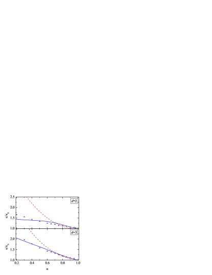
Figure 1: (Color online) Plot of the (reduced) thermal conductivity $\kappa/\kappa_{0}$ as a function of $\alpha$ for hard disks (top panel) and hard spheres (bottom panel). The dashed and solid lines represent the standard and modified first Sonine approximations, respectively. The symbols are DSMC results obtained from the GK relations BRM04 ; BRMMG05 .

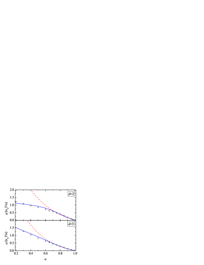
Figure 2: (Color online) Plot of the (reduced) transport coefficient $\mu/(\kappa_{0}T/n)$ as a function of $\alpha$ for hard disks (top panel) and hard spheres (bottom panel). The dashed and solid lines represent the standard and modified first Sonine approximations, respectively. The symbols are DSMC results obtained from the GK relations BRM04 ; BRMMG05 .

Since both $\kappa$ and $\mu$ are overestimated by the standard approximation, it could happen that, by a cancelation of errors, the transport coefficient $\kappa^{\prime}=\kappa-n\mu/2T$ might be well captured by that approximation. However, this is not the case. The comparison between the computer simulations for $\kappa^{\prime}$ obtained from the two alternative methods of Refs. BRMMG05 and MSG06 and the two theoretical approaches is shown in Fig. 3. As in the cases of $\kappa$ and $\mu$, the modified Sonine approximation for $\kappa^{\prime}$ agrees quite well with the simulation results.

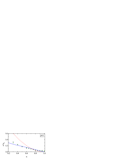
Figure 3: (Color online) Plot of the (reduced) modified thermal conductivity $\kappa^{\prime}/\kappa_{0}$ as a function of $\alpha$ for hard spheres. The dashed and solid lines represent the standard and modified first Sonine approximations, respectively. The symbols are DSMC results obtained from the GK relations BRMMG05 (triangles) and from the application of an external force MSG06 (circles).

The good agreement found in Figs. 1–3 between the modified first Sonine approximation and the simulation data for the heat flux transport coefficients suggests that the NS distribution functions $\bm{\mathcal{A}}(\mathbf{V})$ and $\bm{\mathcal{A}}^{\prime}(\mathbf{V})$ are well represented by the forms (23). To test this expectation, we compare now the standard and modified Sonine approximations for $\bm{\mathcal{A}}^{\prime}(\mathbf{V})$ with simulation data presented in Ref. MSG06 for the three-dimensional case. By symmetry arguments, the function $\bm{\mathcal{A}}^{\prime}(\mathbf{V})$ can be written as

$$\bm{\mathcal{A}}^{\prime}(\mathbf{V})=\lambda v_{0}^{-1}f_{M}(\mathbf{V})\Phi(c^{2})\mathbf{V},$$ (34)

where $\lambda=1/\sqrt{2}\pi n\sigma^{2}$ is the mean free path, $v_{0}=\sqrt{2T/m}$ is the thermal speed, and $\Phi(c^{2})$ is a dimensionless isotropic function of the scaled velocity $\mathbf{c}={\mathbf{V}}/{v_{0}}$. All the information contained in $\Phi(c^{2})$ is retained by the marginal distribution MSG06

$$\varphi(c_{x}^{2})=\pi^{-1}\int_{-\infty}^{\infty}dc_{y}\int_{-\infty}^{\infty}dc_{z}\,e^{-(c_{y}^{2}+c_{z}^{2})}\Phi(c^{2}).$$ (35)

According to the standard approximation (14),

$$\Phi(c^{2})=\frac{4\kappa^{\prime}}{5n\lambda v_{0}}\left(\frac{5}{2}-c^{2}\right),$$ (36)

so that

$$\varphi(c_{x}^{2})=\frac{4\kappa^{\prime}}{5n\lambda v_{0}}\left(\frac{3}{2}-c_{x}^{2}\right).$$ (37)

In contrast, the modified approximation (23) yields,

$$\Phi(c^{2}) = \frac{4\kappa^{\prime}}{5n\lambda v_{0}}\left[1+\frac{a_{2}}{2}\left(c^{4}-5c^{2}+\frac{15}{4}\right)\right]\frac{\frac{5}{2}(1+a_{2})-c^{2}}{1+\frac{11}{2}a_{2}}$$ (38)

$$= \frac{4\kappa^{\prime}}{5n\lambda v_{0}}\left[\frac{5}{2}-c^{2}+a_{2}\left(\frac{105}{16}+\frac{21}{8}c^{2}\right.\right.$$

$$\left.\left.-\frac{15}{4}c^{4}+\frac{1}{2}c^{6}\right)\right],$$

where in the last equality we have neglected nonlinear terms in $a_{2}$. The corresponding marginal distribution is

$$\varphi(c_{x}^{2})=\frac{4\kappa^{\prime}}{5n\lambda v_{0}}\left[\frac{3}{2}-c_{x}^{2}-a_{2}\left(\frac{75}{16}-\frac{15}{8}c_{x}^{2}-\frac{9}{4}c_{x}^{4}+\frac{1}{2}c_{x}^{6}\right)\right].$$ (39)

The function $\varphi(c_{x}^{2})$ is plotted in Fig. 4 for $\alpha=0.5$ and $\alpha=0.3$. We see that the modified first Sonine distribution (39) captures reasonably well the main features of the true distribution, especially for $\alpha=0.5$. On the other hand, the standard first Sonine distribution (37) strongly disagrees with the simulation data for $c_{x}^{2}\gtrsim 6$. This velocity region has a significant influence on the evaluation of the thermal conductivity at high inelasticity MSG06 .

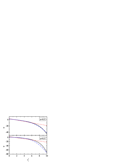
Figure 4: (Color online) Plot of the marginal distribution function $\varphi(c_{x}^{2})$ obtained from DSMC (solid lines) for $\alpha=0.5$ (top panel) and $\alpha=0.3$ (bottom panel). The dashed and dotted-dashed lines represent the standard and modified first Sonine approximations, respectively.

IV.2 Pressure tensor

Although the $\alpha$-dependence of the shear viscosity is well described by the standard first Sonine approximation, it is worthwhile comparing the modified first Sonine estimate against computer simulations. To the best of our knowledge, the NS shear viscosity has been measured in DSMC simulations by three alternative methods: (i) by analyzing the time decay of a weak transverse shear wave in the HCS BRMC99 ; (ii) from the GK relation BRM04 ; BRMMG05 ; and (iii) by the application of a homogeneous external force MSG05 . The simulation data obtained by these methods and the two theoretical approximations are presented in Fig. 5. The data obtained from the method (i) are restricted to $d=3$ and $\alpha\geq 0.7$ BRMC99 , while the ones from the method (ii) are available for $d=2$ BRM04 and $d=3$ BRMMG05 . Regarding the method (iii), the data corresponding to $d=3$ for $\alpha\geq 0.6$ were reported in Ref. MSG05 , while those corresponding to $d=3$ for $\alpha\geq 0.5$ and to $d=2$ have been obtained in this work. We observe that up to $\alpha\simeq 0.6$ the simulation data are consistent among themselves and also with both theories. However, for higher inelasticities, there is a certain discrepancy (less than 10%) between the data reported in Refs. BRM04 ; BRMMG05 and those presented here, the former being close to the standard estimates and the latter being close to the modified estimates, especially in the three-dimensional case. The small difference between our simulation data and those of Refs. BRM04 ; BRMMG05 might be due to the influence of velocity correlations in the correlation function involved in the GK expression of the shear viscosity. These velocity correlations are larger than in the case of the heat-flux transport coefficients BRM04 .

Figure 5: (Color online) Plot of the (reduced) shear viscosity $\eta/\eta_{0}$ as a function of $\alpha$ for hard disks (top panel) and hard spheres (bottom panel). The dashed and solid lines represent the standard and modified first Sonine approximations, respectively. The symbols are DSMC results obtained from the decay of a sinusoidal perturbation BRMC99 (squares), from the GK relations BRM04 ; BRMMG05 (triangles), and from the application of an external force MSG05 (circles). In the latter case, the data corresponding to $d=3$ for $\alpha\leq 0.5$ and to $d=2$ have been obtained in the present work.

In conclusion, while the standard first Sonine approximation does quite good a job for the shear viscosity, it is fair to say that the modified approximation is still better, especially for three-dimensional systems.

IV.3 Self-diffusion

Finally, we consider the self-diffusion coefficient. This coefficient has been measured in computer simulations from the mean square displacement of a tagged particle in the HCS BRMCGR00 ; LBD02 ; GM04 , as well as by the decay of a sinusoidal perturbation in the concentration of tagged particles BRMCGR00 . We observe in Fig. 6 that both Sonine approximations provide a general good agreement with simulation data. However, the standard approximation slightly overestimates the self-diffusion coefficient at high inelasticity, this effect being corrected again by the modified approximation.

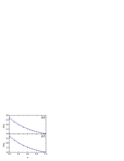
Figure 6: (Color online) Plot of the (reduced) self-diffusion coefficient $D/D_{0}$ as a function of $\alpha$ for hard disks (top panel) and hard spheres (bottom panel). The dashed and solid lines represent the standard and modified first Sonine approximations, respectively. The symbols are computer simulation results obtained from the mean square displacement. In the top panel, the triangles correspond to molecular dynamics results BRMCGR00 and the circles are DSMC results obtained in the present work. In the bottom panel, the triangles are DSMC results reported in Ref. BRMCGR00 and the circles are DSMC results presented in Ref. GM04 ($\alpha\geq 0.6$) and obtained in the present work ($\alpha\leq 0.5$).

V Concluding remarks

This work has been mainly motivated by the disagreement found at high dissipation between the simulation data for the heat flux transport coefficients and the expressions derived from the standard first Sonine approximation BRM04 ; BRMMG05 ; MSG06 . Although this disagreement appears beyond the region of inelasticity of practical interest, it is physically relevant from a fundamental point of view to propose alternative theoretical approaches that correct the limitations of the standard approximation. Here, we have implemented a modified version (23) of the first Sonine approximation (14), where the weight function is no longer the Maxwell–Boltzmann distribution $f_{M}$ but the HCS distribution $f^{(0)}$. Moreover, in order to preserve the solubility conditions, the polynomial $\mathbf{S}(\mathbf{V})$ defined by Eq. (8) must be replaced by the modified polynomial $\overline{\mathbf{S}}(\mathbf{V})$ defined by Eq. (25). The idea behind the modified method is that the deviation of $f^{(0)}$ from $f_{M}$ has an important influence on the NS distribution $f^{(1)}$, so that the latter is better captured by the approximation (23) than by the approximation (14). In other words, the rate of convergence of the polynomial expansion is expected to be accelerated when $f^{(0)}$ rather than $f_{M}$ is used as weight function.

The structure of the transport coefficients is common in both approximations. They are given by Eqs. (2)–(4) and (10). However, the $\alpha$-dependence of the characteristic collision frequencies differs in both methods. In the standard first Sonine approximation, those collision frequencies are given by Eqs. (20)–(22), while they are given by Eqs. (30)–(32) in the modified first Sonine approximation. It is apparent that the distinction between both approximations occurs in the value of the coefficient of the fourth cumulant $a_{2}$. In the standard approximation that coefficient comes from the dependence of the linearized Boltzmann collision operator on $f^{(0)}$ only, while in the modified approximation it also comes from the assumed form for $f^{(1)}$. The effect of the latter contribution becomes more important than that of the former, so that, for each collision frequency, the coefficient of $a_{2}$ changes dramatically from the standard approximation to the modified one.

As observed in Figs. 1–3, the modified approximation significantly improves the $\alpha$-dependence of $\kappa$, $\mu$, and the difference $\kappa^{\prime}=\kappa-n\mu/2T$. This is the primary result of this paper. Additionally, as shown in Figs. 5 and 6, the slight discrepancies between simulation and the standard first Sonine estimates for the shear viscosity $\eta$ and the self-diffusion coefficient $D$ are partially corrected by the modified approximation.

Although the results reported here have been restricted to a low-density granular gas described by the inelastic Boltzmann equation, they can be straightforwardly extended to finite density in the framework of the Enskog kinetic theory. In that case, application of the CE method shows that the effective collision frequencies are the same as in the dilute limit, except for a density-dependent factor $\chi$ GD99 ; L05 . The explicit expressions for the NS transport coefficients are presented in Appendix B. We expect that these Enskog results can stimulate the performance of molecular dynamics simulations to test whether or not the modified first Sonine approximation improves again over the predictions of the standard approximation, especially in the case of the heat flux transport coefficients at high inelasticity.

Appendix A Modified polynomial expansion

Given a weight function

$$w(x)=e^{-x}\left[1+\sum_{k=2}^{\infty}a_{k}L_{k}^{(p-1)}(x)\right],$$ (40)

the mathematical problem consists of finding a set of polynomials $\{\overline{L}_{k}^{(p)}(x)\}$ such that they are mutually orthogonal with respect to the scalar product

$$(f_{1},f_{2})=\int_{0}^{\infty}dx\,x^{p}w(x)f_{1}(x)f_{2}(x).$$ (41)

If $a_{k}=0$, then $w(x)=e^{-x}$ and one has the Laguerre polynomials, i.e., $\overline{L}_{k}^{(p)}(x)={L}_{k}^{(p)}(x)$. In the general case, the polynomials $\overline{L}_{k}^{(p)}(x)$ can be obtained following the Gram–Schmidt orthogonalization procedure. Suppose the polynomials $\overline{L}_{\ell}^{(p)}(x)$ with $\ell\leq k-1$ are already known. The next unknown polynomial can be written as

$$\overline{L}_{k}^{(p)}(x)=c_{k}^{(k)}x^{k}+\sum_{\ell=0}^{k-1}c_{\ell}^{(k)}\overline{L}_{\ell}^{(p)}(x),$$ (42)

where the coefficients $c_{\ell}^{(k)}$ are to be determined. One of them can be fixed by the standardization condition. For instance, we can take $c_{k}^{(k)}=(-1)^{k}/k!$, which is the same coefficient as in ${L}_{k}^{(p)}(x)$. The orthogonalization condition $(\overline{L}_{\ell}^{(p)},\overline{L}_{k}^{(p)})=0$ for $\ell\leq k-1$ gives

$$c_{\ell}^{(k)}=-c_{k}^{(k)}\frac{(\overline{L}_{\ell}^{(p)},x^{k})}{(\overline{L}_{\ell}^{(p)},\overline{L}_{\ell}^{(p)})}.$$ (43)

This closes the construction of $\overline{L}_{k}^{(p)}(x)$ and the process can be recursively continued. Since $\overline{L}_{k-1}^{(p)}(x)x^{k+1}$ is a polynomial of degree $2k$, and given the orthogonality properties of the Laguerre polynomials $L_{k}^{p-1}(x)$ appearing in the representation (40), it is straightforward to see that only the first $k$ coefficients $\{a_{\ell},\ell\leq k\}$ appear in $\overline{L}_{k}^{(p)}(x)$. The norm of $\overline{L}_{k}^{(p)}(x)$, however, involves the coefficient $a_{2k+1}$.

The three first polynomials are $\overline{L}_{0}^{(p)}(x)=1$,

$$\overline{L}_{1}^{(p)}(x)=(p+1)(1+a_{2})-x,$$ (44)

$$\overline{L}_{2}^{(p)}(x)=\frac{1}{2}x^{2}+c_{0}^{(2)}+c_{1}^{(2)}\overline{L}_{1}^{(p)}(x),$$ (45)

where

$$c_{0}^{(2)}=-\frac{p^{2}+3p+2}{2}(1+3a_{2}-a_{3}),$$ (46)

$$c_{1}^{(2)}=\frac{p+2}{2}\frac{2+2(p+7)a_{2}-(p+1)a_{2}(3a_{2}-a_{3})-(3p+11)a_{3}+(p+3)a_{4}}{1+(p+4)a_{2}-(p+1)a_{2}^{2}-(p+2)a_{3}}.$$ (47)

Appendix B Transport coefficients for a dense granular gas

In this Appendix, we give the expressions for the NS transport coefficients obtained from the Enskog kinetic equation by the application of the CE method GD99 ; L05 in the first Sonine approximation.

The bulk viscosity (which vanishes in the dilute limit) is

$$\gamma=\eta_{0}\frac{2^{2d+1}}{(d+2)\pi}\phi^{2}\chi(1+\alpha)\left(1-\frac{1}{16}a_{2}\right),$$ (48)

where

$$\phi\equiv\frac{\pi^{d/2}}{2^{d}\Gamma(1+d/2)}n\sigma^{d}$$ (49)

is the solid volume fraction and $\chi(\phi)$ is the pair correlation function at contact. The shear viscosity $\eta$ has a kinetic part $\eta^{k}$ and a collisional part $\eta^{c}$, where

$$\eta^{k}=\frac{\eta_{0}}{\chi}\left(\nu_{\eta}^{*}-\frac{1}{2}\zeta^{*}\right)^{-1}\left[1-\frac{2^{d-2}}{d+2}(1+\alpha)(1-3\alpha)\phi\chi\right],$$ (50)

$$\eta^{c}=\frac{2^{d-1}}{d+2}\phi\chi(1+\alpha)\eta^{k}+\frac{d}{d+2}\gamma.$$ (51)

Analogously, the coefficients associated with the heat flux have also kinetic and collisional contributions. They are

$$\kappa^{k} = \frac{\kappa_{0}}{\chi}\frac{d-1}{d}\left(\nu_{\kappa}^{*}-2\zeta^{*}\right)^{-1}\Bigl{\{}1+2a_{2}$$

$$+3\frac{2^{d-3}}{d+2}\phi\chi(1+\alpha)^{2}\left[(1+\alpha)a_{2}-1+2\alpha\right]\Bigr{\}},$$

$$\kappa^{c} = 3\frac{2^{d-2}}{d+2}\phi\chi(1+\alpha)\kappa^{k}+\frac{2^{2d+1}(d-1)}{(d+2)^{2}\pi}\phi^{2}\chi(1+\alpha)$$ (53)

$$\times\left(1+\frac{7}{16}a_{2}\right)\kappa_{0},$$

$$\mu^{k} = \frac{T}{n}\frac{\kappa_{0}}{\chi}\left(\nu_{\kappa}^{*}-\frac{3}{2}\zeta^{*}\right)^{-1}\left\{\frac{\kappa^{k}}{\kappa_{0}}\xi\zeta^{*}+\frac{d-1}{d}a_{2}\right.$$

$$\left.+3\frac{2^{d-3}(d-1)}{d(d+2)}\phi(\chi+\xi)(1+\alpha)\right.$$

$$\left.\times\left[\frac{1}{6}(3\alpha^{2}-3\alpha+10+2d)a_{2}-\alpha(1-\alpha)\right]\right\},$$

$$\mu^{c}=\mu^{k}3\frac{2^{d-2}}{d+2}\phi\chi(1+\alpha).$$ (55)

In Eq. (LABEL:B8), we have introduced the quantity $\xi\equiv\partial(\phi\chi)/\partial\phi$.

Finally, the self-diffusion coefficient is simply given by

$$D=\frac{D_{0}}{\chi}\frac{d+2}{2d}\frac{1}{\nu_{D}^{*}-\frac{1}{2}\zeta^{*}}.$$ (56)

In the above equations, $\eta_{0}$, $\kappa_{0}$, and $D_{0}$ are the elastic values of the low-density shear viscosity, thermal conductivity, and self-diffusion coefficient, respectively. They are given by

$$\eta_{0}=\frac{nT}{\nu_{0}},\quad\kappa_{0}=\frac{d(d+2)}{2(d-1)}\frac{\eta_{0}}{m},$$ (57)

$$D_{0}=\frac{2d}{d+2}\frac{T}{m\nu_{0}},$$ (58)

where the collision frequency $\nu_{0}$ is defined by

$$\nu_{0}=\frac{8}{d+2}\frac{\pi^{(d-1)/2}}{\Gamma(d/2)}n\sigma^{d-1}\left(\frac{T}{m}\right)^{1/2}.$$ (59)

In addition, the reduced cooling rate $\zeta^{*}$ for a dilute gas in the HCS is given by Eq. (12).

The expressions (50)–(56) are common to the standard and the modified first Sonine approximations. However, as discussed in the main text, they differ in the $\alpha$-dependence of the (reduced) effective collision frequencies $\nu_{\eta}^{*}$, $\nu_{\kappa}^{*}$, and $\nu_{D}^{*}$, which are given by Eqs. (20)–(22) in the standard approximation and by Eqs. (30)–(32) in the modified one. Note that, since the collisional contributions depend on their kinetic counterparts, they also differ in both approximations.

References

- (1) C. S. Campbell, Annu. Rev. Fluid Mech. 22 (1990) 57; I. Goldhirsch, ibid. 35 (2003) 267 .
- (2) N. V. Brilliantov and T. Pöschel, Kinetic Theory of Granular Gases, Oxford University Press, Oxford, 2004.
- (3) J. J. Brey, J. W. Dufty, C. S. Kim, and A. Santos, Phys. Rev. E 58 (1998) 4638.
- (4) V. Garzó and J. W. Dufty, Phys. Rev. E 59 (1999) 5895.
- (5) J. J. Brey and D. Cubero, in Granular Gases, edited by T. Pöschel and S. Luding, Springer-Verlag, Berlin, 2001, pp. 59–78.
- (6) V. Garzó and J. W. Dufty, Phys. Fluids 14 (2002) 1476.
- (7) J. F. Lutsko, Phys. Rev. E 72 (2005) 021306.
- (8) J. J. Brey, M. J. Ruiz-Montero, and D. Cubero, Europhys. Lett. 48 (1999) 359.
- (9) J. J. Brey, M. J. Ruiz-Montero, D. Cubero, and R. García-Rojo, Phys. Fluids 12 (2000) 876.
- (10) J. Lutsko, J. J. Brey, and J. W. Dufty, Phys. Rev. E 65 (2002) 051304.
- (11) V. Garzó and J. M. Montanero, Physica A 313 (2002) 336.
- (12) J. M. Montanero and V. Garzó, Phys. Rev. E 67 (2003) 021308.
- (13) V. Garzó and J. M. Montanero, Phys. Rev. E 69 (2004) 021301.
- (14) J. J. Brey and M. J. Ruiz-Montero, Phys. Rev. E 70 (2004) 051301.
- (15) J. J. Brey, M. J. Ruiz-Montero, P. Maynar, and M. I. García de Soria, J. Phys.: Condens. Matter 17 (2005) S2489.
- (16) J. M. Montanero, A. Santos, and V. Garzó, in Rarefied Gas Dynamics: 24th International Symposium on Rarefied Gas Dynamics, edited by M. Capitelli, AIP Conference Proceedings, vol. 762, Melville, NY, 2005, pp. 797–802; preprint arXiv: cond-mat/0411219.
- (17) J. M. Montanero, A. Santos, and V. Garzó, First-order Chapman–Enskog velocity distribution function in a granular gas, Physica A (to be published).
- (18) G. Bird, Molecular Gas Dynamics and the Direct Simulation of Gas Flows, Clarendon, Oxford, 1994; F. J. Alexander and A. L. Garcia, Comp. Phys. 11 (1997) 588.
- (19) J. J. Brey and D. Cubero, Phys. Rev. E 57 (1998) 2019.
- (20) A. Santos, V. Garzó, and J. W. Dufty, Phys. Rev. E 69 (2004) 061303.
- (21) A. Goldshtein and M. Shapiro, J. Fluid Mech. 282 (1995) 75.
- (22) J. J. Brey, J. W. Dufty, and A. Santos, J. Stat. Phys. 87 (1997) 1051.
- (23) S. Chapman and T. G. Cowling, The Mathematical Theory of Nonuniform Gases, Cambridge University Press, Cambridge, 1970.
- (24) T. P. C. van Noije and M. H. Ernst, Gran. Matt. 1 (1998) 57.
- (25) J. M. Montanero and A. Santos, Gran. Matt. 2 (2000) 53.
- (26) F. Coppex, M. Droz, J. Piasecki, and E. Trizac, Physica A 329 (2003) 114.
- (27) V. Garzó and A. Santos, Kinetic Theory of Gases in Shear Flows. Nonlinear Transport, Kluwer Academic Publishers, Dordrecht, 2003.
- (28) For details, see Appendix A of arXiv: cond-mat/0604079 v1.
- (29) J. J. Brey, D. Cubero, and M. J. Ruiz-Montero, Phys. Rev. E 59 (1999) 1256.
- (30) N. V. Brilliantov and Pöschel, Europhys. Lett. 74 (2006) 424; Erratum: 75 (2006) 188.
- (31) J. W. Dufty and J. J. Brey, J. Stat. Phys. 109 (2002) 433.