Density Matrix Renormalization Group study on incommensurate quantum Frenkel-Kontorova model
Abstract
By using the density matrix renormalization group (DMRG) technique, the incommensurate quantum Frenkel-Kontorova model is investigated numerically. It is found that when the quantum fluctuation is strong enough, the g-function featured by a saw-tooth map in the depinned state will show a different kind of behavior, similar to a standard map, but with reduced magnitude. The related position correlations are studied in details, which leads to a potentially interesting application to the recently well-explored phase transitions in cold atoms loaded in optical lattices.
64.60.Ak, 64.70.Rh, 05.10.Cc, 05.45.-a
I Introduction
As a generic model to demonstrate the fractal “devil’s staircase”, 1D Frenkel Kontorova (FK) model has been investigated extensively in the field of classical nonlinear physics ever since 1970’s. 1 This model describes the dynamics of a chain of particles connected by springs in the presence of a sinusoidal external potential. Its most essential feature is the involvement of two competing length scales. One is the average distance between the particles and the other is the spatial period of the external potential. This characteristics can be demonstrated in various physical systems, such as crystal dislocations,2 epitaxial monolayers on the crystal surface,3 charge density waves 4 and dry frictions 5 et al. Hence studying FK model can lead to the understanding of many universal properties in those realistic systems. For example, in the classical regime, when the ratio of two length scales are rational, i.e. in the commensurate case, any magnitude of external potential will take the particles into pinned state. But for irrational ratio, i.e. in the incommensurate case, only when the external potential is above a threshold can the ground state stay in the pinned state. This later phenomenon is closed related to the breakup of KAM curves into cantorus since the equilibrium positions of the particles are described by the well known Chirikov standard map.6 This is the so-called Transition of Breaking Analyticity (TBA) pioneered by Aubry et al.7 ; 8 ; 9
So far, the classical properties of the 1D FK model have been well understood. As a further step, we need to know how quantum effect will modify those classical results. The research along this line will not only bring us into the topic of the classical-quantum correspondence, but also take us into a fascinating quantum world, where no classical correspondence exists. Unfortunately, until now, there is not much work about it because of the complexes related to the notorious quantum many-body problems. The first work in this direction appeared in 1989,10 in which by using the Feynman path-integral quantization scheme and the Metropolis algorithm, Borgonovi et al. has shown the transition of the g-function from a standard map to a saw-tooth one for incommensurate quantum FK model. Similar results have also been reported by the mean-field theory11 and the squeezed state method.12 ; 13 ; 14 Recently Krajewski et al. has studied the commensurate quantum FK model15 with the algorithm of path-integral molecular dynamics.
In this paper, instead of making use of the known properties of the classical theory as a starting point for the investigations, we attemp to study the quantum FK model directly. The employed technique is the density matrix renormalization group (DMRG) method.16 Since its appearance in 1992,17 through more than one decade of developments,18 DMRG has now become the most powerful and efficient numerical method to solve one-dimensional quantum many-particle systems. A lot of techniques for the efficiency improvement have been put forward. The details of how to apply them upon quantum FK model will be presented in Section III.
Besides the theoretical interest, another motivation for us to carry out this work is the rapid experimental development in trapping and controlling Bose-Einstein condensates by the optical lattices.19 ; Greiner ; Paredes ; 20 Especially, since the seminal experiment by Greiner et al. observing the phase transitions in cold atoms from superfluid (SF) to Mott Insulator (MI),19 the progresses in this field have been explosive. For the moment, one-, two- and three- dimensional quantum systems can be readily created in experiments.Koehl Theoretically, to describe the underlying physics of these experiments, the Bose-Hubbard model and its various extended versions are widely used.21 ; 22 ; 23 But the intrinsic tight-binding approximations often require very strong external potentials. On the other hand, when the external potential is very weak, the quantum sine-Gordon modelColeman might be an optional model so long as the continuum approximation is applicable. Between the two limiting situations, the minimal model should be quantum FK model, which is actually a discrete version of the sine-Gordon model; hence it goes beyond the limit of continuum or hydrodynamic approximations. It is hoped that our work could not only shed some light on the interpretation of the present on-going experiments, but also help to provide some new insights in modeling and designing the future experiments in wider scope.
In the following section, the FK model is presented and transformed to the second-quantized form suitable for the realization of DMRG algorithm. Section 3 explains in detail the DMRG procedures used for quantum FK model. Section 4 is devoted to the results and discussions. In Section V, some physics underlying our calculations are further explored. Finally we will summarize and conclude the work.
II Hamiltonian for quantum FK model
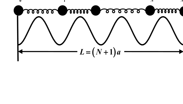
Fig. 1 shows the schematic diagram of the system we study. There are particles connected by springs and put in a 1D external sinusoidal potential, which could be regarded as representing the effect of a loading optical potential. The fixed-boundary condition is used with and , in which , is the coordinate of the th particle and is the average distance between neighbouring particles. The Hamiltonian can be expressed as,
| (1) |
where is the wave number of the external potential, the force constant of the springs and the magnitude of the external potential. By introducing the following dimensionless parameters,
| (2) |
we can rewrite Eq. (1) as,
| (3) |
But Eq. (3) is unwieldly for the realization of DMRG technique. It is necessary to recast it into a second-quantized form. For this purpose, the following substitution is employed,
| (4) |
in which are annihilation and creation operators satisfying the boson communication relationship, i.e., . Then the Hamiltonian in Eq. (1) is finally reduced to,
| (5) |
The above Hamiltonian looks quite similar in appearance to that of a lattice system with bosons tight-bounded to the local potentials and only having the nearest-neighbor “hopping” terms. But the physics is quite different. We will come back to this problem later in this paper.
By examining Eq. (5), it can be easily seen that there are three independent tunable parameters. The first one is the scaled plank constant , which is proportional to the square root of the particle kinetic energy, , in the unit of the particle-particle interaction energy , which could be estimated by assuming the particles to occupy the lowest energy level in a 1D potential with a range around . embodies the magnitude of the quantum influence. Experimentally can be varied by changing the effective mass of the particle or the effective strength of the particle-particle interactions.
The second free parameter is , which measures the strength of the external potential in the unit of . This is a parameter most easily accessible in experiments since it is directly related to the strength of the loading optical lasers. Generally speaking, the above two parameters are of competing effect, namely, tends to delocalize the particles while to localize them, as is easily understandable and will also be seen from our following calculations.
The last parameter in Eq. (5) is , which denotes the commensurability property of the system. Because the commensurate-incommensurate phase transitionbak ; bak1 is not the focus of this paper. is taken to be a fixed irrational number in our work, as conventionally done in literature. It is already well-known that, in classical regime with , if is a rational number, the system will be in a pinned state for an arbitrary external potential. In the incommensurate case, the system can only be in a pinned state when is larger than a critical value ; otherwise it will be in a sliding state. But once we take quantum effect into considerations, the above scenario will be greatly modified. Before going to the details, we will first describe the DMRG procedures used for our calculations in the next section.
III DMRG procedure
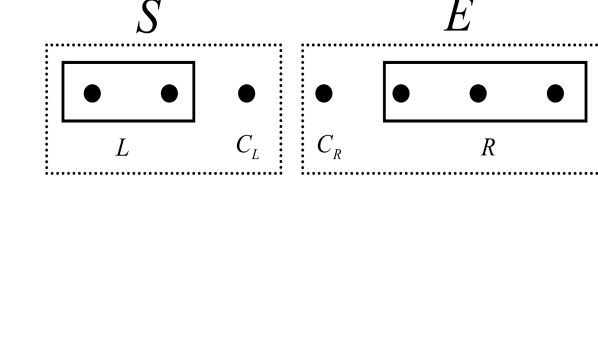
The essential steps of DMRG method are to form a superblock consisted of two parts denoted by and . Then, from the targeted state, for example, the ground state of the superblock, one can obtain the reduced density matrix of by tracing out the component related to , i.e., . Finally by keeping only eigenstates of with the largest eigenvalues, all the operators related to will be rebuilt in the space of reduced dimension . It can be proved that the ground states of the rebuilt has a maximum overlap with the true ground state when is embedded in the superblock. The error is proportional to the sum of the residue eigenvalues thrown away in the rebuilding processes. Due to the exponential decrease of the eigenvalues from for most of the physical systems, very accurate results can still be obtained though working in a much restricted Hilbert space.
Schematically, the ideas behind DMRG can be explained by Fig. 2. The system is composed of left block and left single site . The environment is composed of right block and right single site . It is assumed that the Hilbert space of and have already been truncated to have dimension with bases written as and , respectively. Initially, the dimension for the full Hilbert space of is . Our aim is to seek most effective bases to truncate this full Hilbert space. DMRG technique has provided us an optimal way to realize this aim. For example, we express the targeted state of the superblock as , in which and are the bases of and . Then the most effective states to represent is the eigenvectors of the reduced density matrix with largest magnitude of eigenvalues. Here . Once the Hilbert space for is truncated in this way, one can add one more single site into to make a bigger system and then follow the same procedure to make the truncations. Thus step by step, the system size becomes bigger and bigger, while the dimension for the effective Hilbert space keeps to be . This is the so-called infinite algorithm in DMRG language. For finite system of fixed number of particles, as the size of grows bigger, will correspondingly becomes smaller. When reaches the end of the whole system, we will change the role of and . The truncation procedures are then carried out in the reverse direction along the chain until we get to the other end. This kind of forward and backward ”sweeping” processes can be repeated many times. It is the so-called finite algorithm, which is critical to obtain convergent results in DMRG calculations.
For the Hamiltonian expressed by Eq. (5), because the infinite dimension of the local Hibert space, we will not only need to iteratively decimate the space of the growing quantum system, but also should make a systematic truncation over the local Hibert space. The detailed procedures are summarized as follows.
-
1.
The Hamiltonian in the local Hilbert space is solved numerically for each single particle with the dimension truncated to be ,
(6) in which the local basis set for th particle in the Fock space is expressed as . In coordinate representation,
(7) with to be the Hermite function of order . Using energy as a weighing measure, only states , with the lowest eigen-energy of Eq. (6) are retained to form the working space in the following steps. It should be mentioned that when solving , the following matrix element is used,
(8) by using,
(9) and
(10) -
2.
Carry out the finite-size DMRG algorithm with sweeping. The expounding of the corresponding technical details in this step can be found in many papers or books.16 ; 18 We will not repeat it here. Only some specific techniques adopted in our work are presented as follows.
-
(a)
Conventionally, the superblock in DMRG work is composed of two blocks at the left and right ends together with two single sites in between, which can be schematically expressed as . If the number of retained states for each block is , the dimension for the superblock would be . With , it would be an exceedingly intensive calculation to solve a matrix repeatedly in the sweeping process. So we will use scheme as done in Ref. 30 since now we only need to solve a matrix for the superblock. The amount of calculations are much reduced.
-
(b)
During the warmup processes with the infinite DMRG algorithm before sweeping, the bases for the superblock is selected according to the energy cut-off measure.wei
-
(c)
Once having obtained the solution of the superblock Hamiltonian, the bases of the central site are updated by the eigenstates of the density matrix with the neighboring block parts reduced, i.e., . If we express the bases of left, central and right parts of the superblock by , respectively, according to the decreasing order of the eigenvalues from the corresponding reduced density matrix, we can further reduce the dimension of the superblock by keeping only the basis satisfying . Then the superblock matrix size could be decimate again from to . For example, if is taken to be , we will have a matrix of size instead of . The effectiveness of this technique has been demonstrated in Ref. 32.
-
(a)
-
3.
After obtaining a convergent result in Step 2, higher energy levels from the local Hibert space will be feeded into the systems. To accelerate the calculations, we will feed a group of bases each time. Since the added bases might not be orthogonal to the old ones for each site, all the bases must be orthogonalized and normalized before being submitted to the new round of DMRG sweeping processe in the next step.
-
4.
Continue a new round of DMRG process. But now the central site of the superblock will have a dimension of . As explained in Step 2(b), the same size-cut technique for the superblock is used once again. It should be mentioned that the procedures adopted in Step 3 and Step 4 is based upon the “optimized phonon approach” , which is often used in applying DMRG algorithm for models involving phonons.wei ; wei1 ; zhang ; fried But because Eq. (5) is inhomogeneous along the FK chain, the calculations here are much more intensive than those, for example in Holstein model.zhang We have to calculate the effective phonon bases for each particle individually since no translation or other symmetries can be used.
-
5.
Repeat Step 3 by feeding more extra local basis into the systems until we get convergences in both the decimation of the local Hilbert space and the DMRG sweeping.
-
6.
Goto Step 1 and repeat all the above procedures to ensure the convergence of the results with increasing .
In the following calculations, , and are used. The maximum dimension for the optimized local Hilbert space is , which have been shown to guarantee a numerical convergence. For the test running, we have applied our program upon the exactly solvable model of a pure harmonic chain.caron Very accurate results have been obtained. To spare the space, we will not show the details of the test running and the related comparisons with the analytical results here.
IV Results and discussions
IV.1 Hull function and g-function
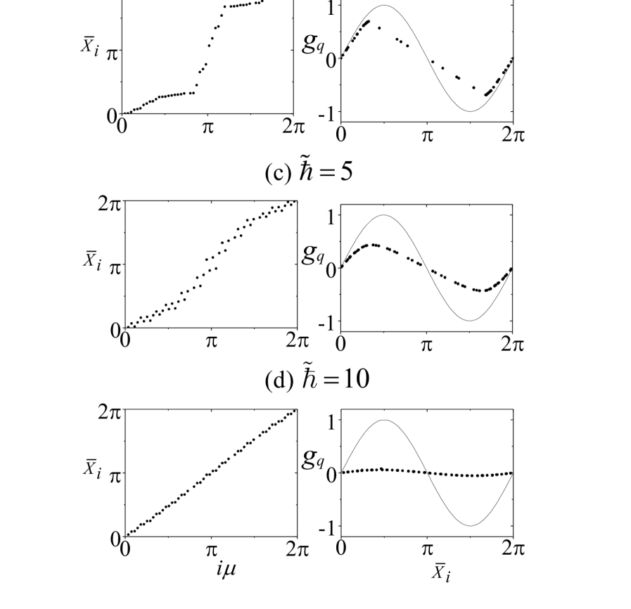
Firstly we check the quantum modifications to the classical hull function and g-function, which are defined in quantum version10 as,
| (11) |
where denote the quantum average of the operator over the ground state . The results are shown in Fig. 3, from which the quantum smoothening effect can be clearly seen. Firstly, when is small, just as expected, there is not much change in the hull and g functions, compared with their classical features, i.e., we have the staircases for the hull function and the discrete points sitting on a sine-function curve for g-function. As increases until a magnitude around , the particles will sample more and more classically-forbidden points along the chain. At the same time, the g-function evolves from a form of standard map to a form of saw-tooth map. These results are consistent with those already found in literature.10 ; 11 ; 12 ; 13 ; 14 From another point of view, they also demonstrates the reliability of our numerical codes.
The most interesting phenomenon takes place in Fig. 3(c) and 3(d), namely, as increases further, the saw-tooth map will become more smoothened and appear in a form similar to a standard map but with a reduced magnitude. Actually, this effect has already shown signs of its existence in the early work from Borgonovi.bor But the fuzzy scattered numerical points there deter a clean justification of the obvervance. In our work, because DMRG algorithm can delve into very large , a clear judgement and detailed study are hence possible. In order to understand what is the underlying physics for this phenomenon, we recall the squeezing state theory,14 which tells us,
| (12) |
where represents the correlation function in particle coordinates, i.e.,
| (13) |
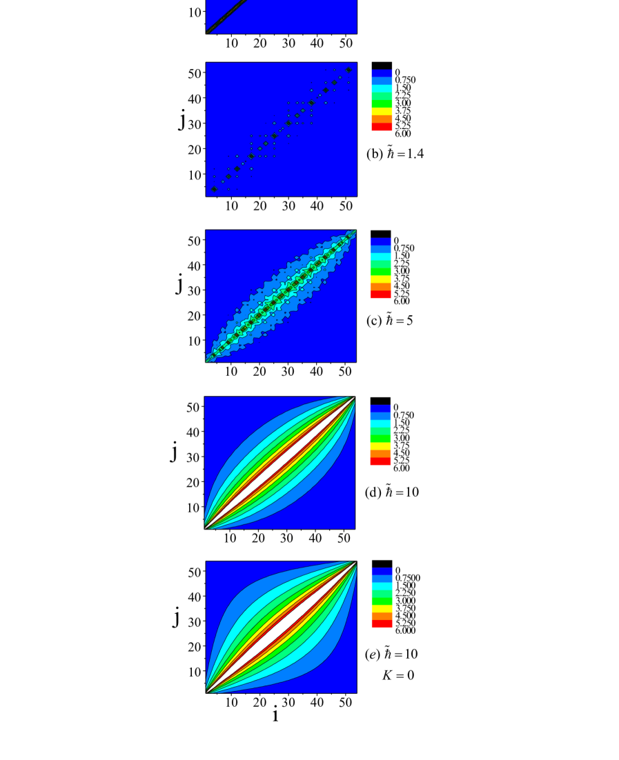
As we know, the squeezed state approach meets an almost insurmmoutable challenge in calculating directly due to the involvement in seeking the periodic orbits in a -dimension map. But the biggest significance of Eq. (12) lies in the fact that it picks up as the most essential physics in understanding the behavior of especially in deep quantum regime. Within DMRG framework, can be derived readily. Fig. 4 presents the contour map of from which three observances are detailed as follows.
-
1.
When is small (), the correlations are confined to a quite narrow region along the diagonal line, which means . So reasonably the system’s behavior is similar to its classical one according to Eq. (12).
-
2.
In the region with around , where a saw-tooth map appears in the -function, we can see some isolated “islands” emerged along the diagonal line in , shown in Fig. 4(b). This means some strong quantum correlations and fluctuations among the individual parts of the chain. This obvious inhomogeneity of with respect to could be regarded as being responsible for the formation of the saw-tooth map.
-
3.
As we explore into the deep quantum region with , a regular pattern of can be observed, which is quite similar to what happens in a pure harmonic chain. For comparisons, we present the case with in Fig. 4(e). The particles are now highly correlated and the previous isolated “islands” merge into each other, which results in a nearly uniform distribution of the diagonal quantum fluctuations. It seems that the quantum fluctuations have strongly renormalized the external potential and make it almost irrelevant as flows to infinity. Consequently, according to Eq. (12), the homogeneity of will drive the saw-tooth map to the standard-map-like one, but with reduced magnitude.
Now we can produce a physical picture underlying the evolution of with respect . In the weak-quantum regime, the particles almost have no correlations. In the middle-quantum regime, the particles start to get correlated with each other from some individual parts of the systems, characterized by the “islands” in the countour map of . When more and more particles becomes correlated, those “islands” will get denser and denser until finally they merge into each other and the systems enter a highly-quantum regime. Since the quantum correlations are closed related to the tunnelling effect, the specific pattern of in the middle quantum regime featured by the saw-tooth map could possibly imply the instanton glass phase ever discussed by Zhirov.24 But because our present algorithm is restricted to the static ground state, it is very difficult to make the direct investigation of this relationship before we can produce the real-time evolution of the systems. Recently the real-time DMRG (RTDMRG) simulation has attracted wide attentions and achieved a lot of progresses.25 It will be our next task to extend the present program to explore the dynamic properties of quantum FK model.
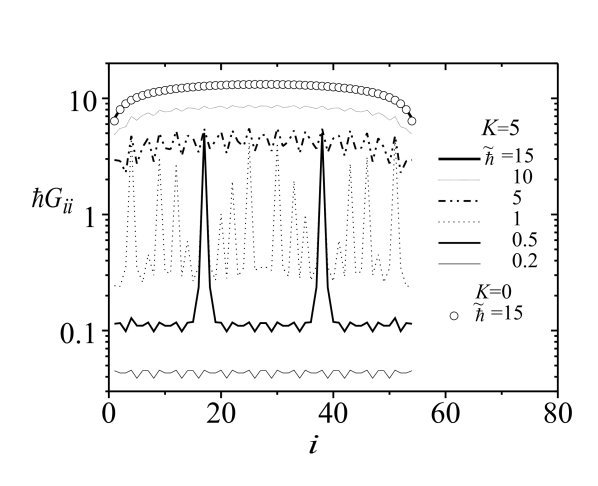
In the above discussions, we have seen that the particle coordinate fluctuation is a very important quantity to characterize the system dynamics under the quantum influences. For brevity, Fig. 5 presents directly the variation of with respect to for different . The “islands” observed in Fig. 4 now becomes peaks. Correspondingly, the special feature in the contour map of also appears in Fig. 5. We will not repeat it here. The interesting effect needed to be noted in Fig. 5 is that, for , the curve almost coincide with that for a harmonic chain with . It tells us that in the deep quantum region, the external potential plays a negligible role for the system behavior, which corroborates once again the reason for the diminishing amplitude in the -function.
IV.2 Average fixed-distance correlations
Because there is no translational symmetry in the incommensurate FK systems, the following average fixed-distance correlations are defined,
| (14) |
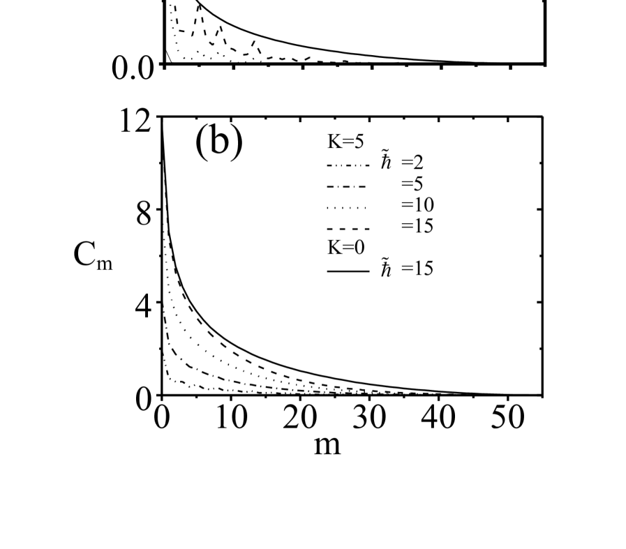
Fig. 6 presents the numerical results of . For comparison, the results for a harmonic model without external potential is also plotted. From Fig. 6, we can address three points. Firstly, for small , there are very little correlations between particles, which approaches their classical behavior in the limit with . Secondly, with increasing , longer-range particle correlations appear. But instead of monotonous decrease over the particle separation as demonstrated by the harmonic model, there appear fluctuations in the curve. This happens just in the parameter range where saw-tooth map effect emerges. Thirdly, as goes beyond about , the curves are getting much smoother without any oscillations until finally approaches the situation without the external potential. But even in the extremely quantum regime, for example , is still smaller than that in the harmonic model except in the short-separation region. This is a bit different from the results shown in Fig. 5, where nice coincidence of the on-site fluctuations is observed. One reason might be that, compared with the accurate calculations of the ground state energy, there is less precision in calculating the correlations with DMRG algorithm and more over DMRG normally under-estimate the particle correlations. . Another reason is that we are here only considering a finite-size chain. When the distance is as large as the system size, it is understandable to expect higher statistical errors for the long-range correlations
To show the extent of similarity between the FK and the harmonic chains with respect to the particle correlations, we introduce the following order parameter,
| (15) |
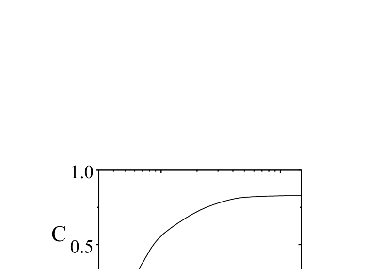
which is just the ratio of the sum for the average fixed-distance correlations in FK chain to that in the harmonic one. Fig. 7 shows the results, from which we see much clearly that as increases, there is a transition region with around . As is large enough, will saturate. The reason for to be smaller than should be the same as explained in the above paragraph.
IV.3 Quantum delocalization effect
Besides the above discussed characteristics of the hull and g-functions, we have also studied the delocalization effect of the quantum modifications based upon the particle wave functions. To discuss this properties, the following definitions are used,
| (16) |
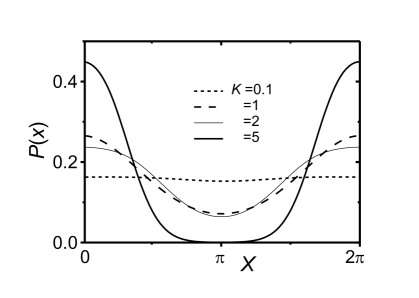
where is the many-particle wave functions of the system, is the probabilities to find the th particle at position and is the total probability to find particles between and . Firstly, let us check the localization effect of the external potential as done in Ref. 14. Fig. 8 shows the numerical results. It can be easily seen that for fixed , as the external potential becomes deeper, the particles will tend to sit near the bottom of the potential until finally all the particles are localized and no particles can be found around the top of the potential. This is the localizing effect of external potential. By defining an order parameter to describe the probability for particles to sit on the potential top,
| (17) |
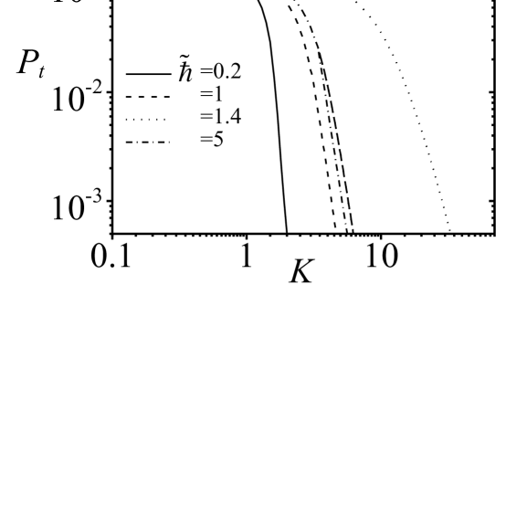
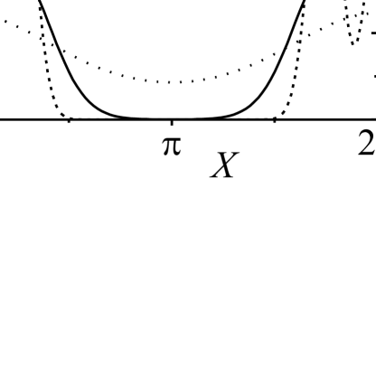
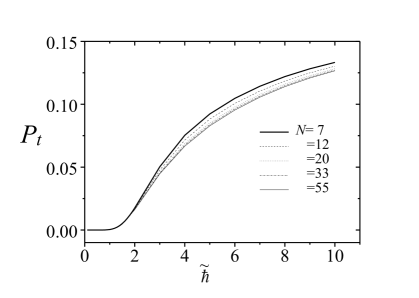
we can find an abrupt jump in the particle localization as shown in Fig. 9. All the results are consistent with those in Hu and Li’s paper.14 As a further work, we continue to explore into the high quantum region by increasing . Fig. 10 presents the function by keeping fixed. It is interesting to note that as increases, more and more particles are found away from the potential bottoms. This is understandable since represents the zero-point kinetic energy of the particles. Once again, we plot the disorder parameter in Fig. 11, from which we see another kind of abrupt change of through a transition region with around , where the probability to locate the particles on the top of the potential suddenly increases. Compared with the localization effect of the external potential, the delocalization effect increases much slower. To check the size-dependence of the results, we have shown the calculations with different in Fig. 11, from which no obvious qualitative change over the above results can be seen. So the quantum delocalization effects seem not much dependent upon the system size. Similar conclusions have also been found in calculating other physical quantities. That is why in most of our work, we only confine to .
V Relevance of quantum FK model to other models
In the above section, we have shown how the quantum effect can greatly modify the classical behavior of a FK chain. In this section, we will further discuss the physical significance of quantum FK model by exploring its relationship with other models.
As already mentioned in the introduction, quantum FK model is a minimal model to describe a system of cold atoms loaded in an optical lattice between two limiting cases: one is the Bose-Hubbard model with tight-binding approximations and the other is the quantum sine-Gordon model with hydrodynamic approximations. The marking parameter for these models can be represented by , which is actually the ratio of the external potential to the kinetic energy of the particles. In the following, we will demonstrate how quantum FK Hamiltonian Eq. (5) looks like with flows to and .
Firstly, as , this situation can be realized by taking with fixed or with fixed. Both options mean that the particles are tight-bounded by the external potential. Hence the particle index can be taken as the lattice site index. Once this connection is built, we will try to expand in Eq. (5) with respect to by taking . To simplify the notation, is used for the expansion. By utilizing the Baker - Campbell - Hausdorff formula under the condition , we can have
| (18) | |||||
The complicated factors in the above sum represents different orders of interactions among the local oscillators through the media of the external potential. We will keep only the terms up to the order of . Further more, with random phase approximations (RPA), only the operator products and are retained. Then Eq. (5) is reduced to,
| (19) |
which is stimulatingly similar in form to the following Bose-Hubbard model with disorders,
| (20) |
where denotes the hopping interaction, is the on-site repulsion, describes the random external potential and is the chemical potential. If we further assume no phase coherence between and , Eq. (19) and Eq. (20) will appear exactly the same except the fixed in Eq. (20). This implicates that we can use very similar mathematical technique to solve both Hamiltonians. But these similarities are only valid literally since the underlying physics or interpretations are quite different. Eq. (20) is a true tight-binding single-band Hamiltonian. Thus physically, represents the creation of a particle on a definite orbit at the -th site. But in Eq. (19), denotes driving the -th particle onto a local state, , , as shown in Eq. (7). In other words, Eq. (19) is more like an infinite-band model. Because of this basic difference, we cannot map the results concerning , which is related to and , directly to the corresponding ones in Eq. (20).
Now the question becomes, besides as a coordinate operator, what implicates in terms of the language from Bose-Hubbard model. The motivation to put forward this question is because a lot of work has already done in Bose-Hubbard model. So the answer will surely help us to extract more physics from our model by analogy. To get some hint of answering this question, we turn to another limit of the quantum FK model with . One obvious limit is the pure harmonic chain. In Section V, we have already seen this effect in the study of the particle coordinate correlations.
As is well-known, if only the low-energy properties are considered, a universal effective harmonic fluid model can be built for any 1D quantum fluid.haldane For example, if we assume the Hamiltonian of a 1D bosonic quantum fluid to be,
| (21) |
in which is the annihilation operator at position satisfying and . Here, it should be noted that, to keep the notation consistent with that in literature, we have dropped the cap over the operator. To avoid confusions, this notation is only used in the following discussions of this section. By using
| (22) |
with the average particle density and assuming that the long-wavelength zero-point fluctuations of the density has a wavenumnber , and can be treated as conjugate canonical fields,
| (23) |
With these substitutions and approximations, Eq. (21) becomes,haldane
| (24) |
in which is the sound velocity and is a dimensionless parameter determines the quasi-long-range order of the bosonic field. When a sinusoidal external potential is added, the above Hamiltonian turns into the famous quantum sine-Gordon form,bue
| (25) |
where is a parameter measuring the commensurability property of the model. By discretizing Eq. (25), we obtain a FK Hamiltonian,
| (26) |
Compared with Eq. (1), it is obvious that has mapped into and into . By checking Eq. (22) again, we can immediately see that Fig. 4 actually is a display of the phase coherence between different particles of a realistic quantum system described Eq. (21) in low-energy regime. This is a fascinating scenario since and can be readily calculated by DMRG algorithm. Since the phase coherence is a purely quantum effect, we can now provide another interpretation to the physics in Fig. 4 and Fig. 5. Firstly, when is quite small, the particles almost have no phase coherence. Then as becomes larger, the phase correlation pattern makes the system more like a bose glass, which has been widely discussed related to disordered Bose-Hubbard model.fish ; krau ; sca When takes the system into highly quantum regime, all particles are in a phase-coherent state, much like a superfluid state. With these crude qualitative discussions, we are motivated to follow a remarkable way to explore the non-trivial phase diagrams in quantum FK model by investigating the particle coordinate and momentum correlations. This will provide us an interesting and attractive application of our numerical results to the on-going experiments in the field of cold atoms trapped by optical lattices. Further work along this direction will is still in progress and will be presented in another paper.
VI Summary
In summary, for an incommensurate quantum FK model in the supercritical regime, we can divide the effect of the quantum modifications into three categories.
-
1.
When , little alternations can be observed in the hull and functions, compared with their classical behavior. There is negligible phase coherence among the particles.
-
2.
As increases further, for example around when , individual neighbouring particles begin to be highly correlated. During this process, the saw-tooth map will appear to represent the -function.
-
3.
With high enough, more neighboring particles join to strengthen the correlations until all the particles are strongly correlated . At this time, the saw-tooth map will be replaced by a map similar to a standard map, but with much smaller amplitude.
On a qualitative basis, we have shown the relationship of the coordinate correlations calculated in our work to the phase coherence properties in a 1D bosonic system. The interesting variations of the correlation pattern with respect to the quantum modifications could have direct relevance to the interference patterns observed in the superfluid/Mott phase transitions in cold atoms loaded in optical lattices.an The systematic investigation will be the focus of our following work.
This work was supported in part by grants from the Hong Kong Research Grants Council (RGC) and the Hong Kong Baptist University Faculty Research Grant (FRG).
References
- (1) O. M. Braun and Yuri, S. Kivshar, The Frenkel-Kontorova Model:Concepts, Methods, and Applications ( Springer, 2003).
- (2) F. Nabarro, Theory of Crystal Dislocations (Clarendon, Oxford, 1967).
- (3) S. C. Ying, Phys. Rev. B 3, 4160 (1971).
- (4) L. M. Floria and J. J. Mazo, Adv. Phys. 45, 505 (1996).
- (5) L. Consoli, H. J. F. Knops and A. Fasolino, Phys. Rev. Lett. 85, 302 (2000).
- (6) S. Aubry, in Soliton and Condensed matter Physics, edited by A. R. Bishop and T. Schneider (Springer, New York, 1978).
- (7) S. Aubry, Physica D 7, 240 (1983).
- (8) S. Aubry and P. Y. Le Daeron, Physica D 8, 381 (1983).
- (9) R. S. MacKay, J. D. Meiss, and I. C. Percival, Physica D 13, 55 (1984).
- (10) F. Borgonovi, I. Guarneri and D. L. Shepelyansky, Phys. Rev. Lett. 63, 2010 (1989).
- (11) G. P. Berman, E. N. Bulgakov and D. K. Campbell, Phys. Rev. B 49, 8212 (1994).
- (12) B. Hu, B. Li and W. M. Zhang, Phys. Rev. E 58, R4068 (1998).
- (13) B. Hu and B. Li, Europhys. Lett. 46, 655 (1999).
- (14) B. Hu and B. Li, Physica A 288, 81 (2000).
- (15) F. R. Krajewski and M. H. Mueser, J. Chem. Phys. 122, 124711 (2005)
- (16) Density-Matrix Renormalization group, edited by I. Peschel, X. Wang, M. Kaulke and K. Hallberg (Springer, Berlin, 1999).
- (17) S. R. White, Phys. Rev. Lett. 69, 2863 (1992).
- (18) U. Schollwoeck, Rev. Mod. Phys. 77, 259 (2005).
- (19) M. Greiner, O. Mandel, T. Esslinger, T. W. Haensch and I. Bloch , Nature 415, 415 (2002).
- (20) M. Greiner, O. Mandel, T. W. Haensch and I. Bloch, Nature 419, 51(2002).
- (21) B. Paredes, A. Widera, V. Murg, O. Mandel, S. Foelling, I. Cirac, G. V. Shlyapnikov, T. W. Haensch and I. Bloch, Nature 429, 277(2004)
- (22) T. Stoferle, H. Moritz, C. Schori, M. Kohl and T. Esslinger, Phys. Rev. Lett. 92, 130403-1 (2004).
- (23) M. Koehl, H. Moritz, T. Stoeferle, C. Schori, T. Esslinger, J. Low Temp. Phys. 138, 635 (2005).
- (24) D. Jaksch, C. Bruder, J. I. Cirac, C. W. Gardiner and P. Zoller, Phys. Rev. Lett. 81, 3108 (1998).
- (25) T. D. Kuhner and H. Monien, Phys. Rev. B 58, R14741 (1998).
- (26) A. W. Sandvik, Leon Balents, and David K. Campbell, Phys. Rev. Lett. 92, 236401 (2004).
- (27) S. Coleman,Phys. Rev. D 11, 2088 C2097 (1975)
- (28) P. Bak, D. Mukamel, J. Villain, K. Wentowska, Phys. Rev. B 19, 1610 (1979).
- (29) P. Bak, Rep. Prog. Phys. 45, 587 (1982).
- (30) O. V. Zhirov, G. Casati and D. L. Shepelyansky, Phys. Rev. E 67, 056209 (2003).
- (31) S. R. White and Adrian E. Feiguin, Phys. Rev. Lett. 93, 076401 (2004).
- (32) L. G. Caron, S. Moukouri, Phys. Rev. B 56, R8471 (1997).
- (33) A. Weisse, H. Fehske, G. Wellein, A. R. Bishop, Phys. Rev. B 62, R747 (2000).
- (34) A. Weie, G. Wellein, and H. Fehske, arXiv.cond-mat/0104533.
- (35) C. Zhang, E. Jeckelmann, and S. R. White, Phys. Rev. Lett. 80, 2661 (1998).
- (36) B. Friedman, Phys. Rev. B 61, 6701 (2000).
- (37) F. Borgonovi, I. Guarneri and D. Shepelyansky, Z. Phys. B 79, 133 (1990).
- (38) F. D. M. Haldane, Phys. Rev. Lett. 47, 1840 (1981).
- (39) H. P. Buchler, G. Blatter and W. Zwerger, Phys. Rev. Lett. 90, 130401-1(2003).
- (40) M. P. A. Fisher, Peter B. Weichman, G. Grinstein, D. S. Fisher, Phys. Rev. B 40, 546 (1989).
- (41) W. Krauth, N. Trivedi, and D. Ceperley, Phys. Rev. Lett. 67, 2307 (1991).
- (42) R. T. Scalettar, G. G. Batrouni, and G. T. Zimanyi, Phys. Rev. Lett. 66, 3144 (1991).
- (43) J. R. Anglin and W. Ketterle, Nature 416, 211 (2002).
Figure Captions
Figure 1 Schematic diagram of FK model with fixed boundary conditions. There are particles connected by springs. The average distance between the neighboring particles is . and are fixed to be and .
Figure 2 Schematic diagram for a superblock composed of left block , right block , left central site and right central site . and forms the system part while and forms the environment part .
Figure 3 Variations of the quantum hull function and g functions with respect to increasing . . The same set of values for is used for all the other figures except being specially noted. Because the external potential has a period , and are folded onto the interval .
Figure 4 Contour map of the coordinate correlations between the -th and the -th particles. For comparison, the case with and is presented in (e).
Figure 5 The coordinate fluctuations of the -th particle with respect to different quantum influences under a fixed external potential with . As in Fig. 4, the results corresponding to and is also presented for comparisons.
Figure 6 Quantum modifications over the average fixed-distance coordinate correlations of the particles under a fixed external potential with . The case with ( in solid line ) is shown for reference. For clarity, (a) and (b) correspond to different range of . In (a), and in (b), .
Figure 7 Variations of the order parameter with respect to .
Figure 8 Probability distribution under different strengths of the external potential with . The coordinates have been folded onto the region .
Figure 9 Total probability to find the particles on the top of the external potential as a function of for different .
Figure 10 Probability distribution under different strengths of the quantum modifications. As in Figure 7, the coordinates have been folded onto the region .
Figure 11 Total probability to find the particles on the top of the external potential as a function of for different system size .