Spin-orbital gap of multiorbital antiferromagnet

Abstract

In order to discuss the spin-gap formation in a multiorbital system, we analyze an $e_{\rm g}$-orbital Hubbard model on a geometrically frustrated zigzag chain by using a density-matrix renormalization group method. Due to the appearance of a ferro-orbital arrangement, the system is regarded as a one-orbital system, while the degree of spin frustration is controlled by the spatial anisotropy of the orbital. In the region of strong spin frustration, we observe a finite energy gap between ground and first-excited states, which should be called a spin-orbital gap. The physical meaning is clarified by an effective Heisenberg spin model including correctly the effect of the orbital arrangement influenced by the spin excitation.

I Introduction

Exotic properties of low-dimensional antiferromagnets have continued to attract much attention in the research field of condensed matter physics, since strong quantum spin fluctuation destroys classical Néel ordering even at zero temperature, while it leads to various types of quantum disordered states. QSS04 In fact, substantial advances in material synthesis and experimental probes have made it possible to gain deep insights into strange spin-liquid phases and quantum phase transitions in realistic low-dimensional compounds. In particular, a class of spin-gapped antiferromagnets has provided rich macroscopic quantum phenomena such as spin-Peierls transition and impurity-induced magnetic ordering in CuGeO₃, Hase1993 ; Masuda2000 ; Fukuyama1996 ; Onishi2000 and Bose-Einstein condensation of magnons in TlCuCl₃. Oosawa1999 ; Nikuni2000 ; Ruegg2003

Microscopic aspects of the spin-gapped phase in low-dimensional antiferromagnets have been extensively discussed on the basis of the antiferromagnetic (AFM) Heisenberg model. In general, a spin gap is defined as the energy difference between singlet ground and triplet first-excited states. The existence of the finite spin gap can be understood by the concept of a valence-bond state. One typical example is a spin-1/2 Heisenberg zigzag chain. MG1969 ; Haldane1982 ; Tonegawa1987 ; Okamoto1992 ; White1996 In fact, the combined effects of quantum fluctuation and geometrical frustration yield a transition from a gapless spin-liquid phase to a gapped dimer phase. In the gapped dimer phase, a valence bond of neighboring spins is stabilized, but the correlations among the valence bonds are significantly suppressed due to the effect of spin frustration, implying that finite energy is required to excite the valence bond from singlet to triplet.

In experiments, as for a model material of the zigzag spin chain, several compounds have been reported, such as SrCuO₂, Matsuda1995 ; Matsuda1997 Cu(ampy)Br₂, Kikuchi2000 and (N₂H₅)CuCl₃. Hagiwara2001 ; Maeshima2003 However, a candidate material with a significant spin gap has not been found, since the frustration effect is much weak in these materials. In such a circumstance, in order to realize the spin-gapped dimer phase in a region of the strong spin frustration, it is important to explore the way to control the degree of the spin frustration. In this context, it is expected that orbital degree of freedom is a key ingredient to cause highly non-uniform spin exchange interactions. Indeed, since $d$- and $f$-electron orbitals in recently focused materials are spatially anisotropic, the sign and magnitude of spin exchange interactions depend on the relative positions of ions and occupied orbitals. In such a case, we envision that orbital ordering occurs so as to minimize the magnetic energy of the spin system. In fact, we have found that orbital ordering actually relaxes the frustration effect in the exchange interaction due to the spatial anisotropy of relevant orbital, even though the lattice originally exhibits a geometrically frustrated structure. Onishi2005a ; Onishi2005b ; Onishi2006

After the occurrence of orbital ordering, one may naively expect that the system is described by an effective spin system on the frozen background of orbital arrangement. It is true that we can intuitively understand what kind of magnetic correlation develops in the static orbital ordering. However, since spin and orbital degrees of freedom strongly interact with each other at the same energy scale, spin dynamics is influenced by orbital one in principle, unless orbital degree of freedom is completely quenched. Such interplay of spin and orbital dynamics has been discussed for spin-orbital models. Brink1998 ; Bala2001 Here, we point out that even though we observe a spin gap, this would not be a pure spin excitation but includes the changes of both spin and orbital states. The spin gap is definitely given by the energy difference between singlet ground and triplet first-excited states, but the orbital arrangement in the ground and excited states can be different. We believe that it is an intriguing issue to clarify how the spin excitation is described in such a variable background of orbital arrangement.

In this paper, we investigate the spin gap of an $e_{\rm g}$-orbital Hubbard model on a zigzag chain by numerical techniques. Due to the appearance of a ferro-orbital (FO) arrangement, the system can be always regarded as a one-orbital system irrespective of the level splitting. When two orbitals are degenerate, the zigzag chain is decoupled to a double-chain spin system to suppress the spin frustration due to the orbital anisotropy. On the other hand, the orbital anisotropy is controlled by the level splitting, leading to the revival of the spin frustration and a finite spin-excitation gap. However, the orbital arrangement is found to change according to the spin excitation, suggesting an important concept of dynamical interplay between spin and orbital degrees of freedom.

The organization of this paper is as follows. In Sec. II, we describe the model Hamiltonian and numerical techniques. In Sec. III, we show the results of the spin and orbital structures in the ground state. Taking account of the orbital arrangement, we will introduce an effective Heisenberg model. Then, in Sec. IV, we discuss the spin-excited states based on the effective model. Finally, the paper is summarized in Sec. V.

II Model and Method

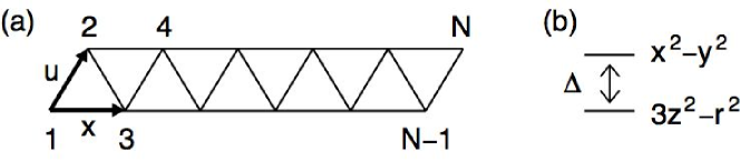
Figure 1: (a) Lattice arrangement and site numbering of $N$-site zigzag chain. (b) Schematic view of level splitting between $e_{\rm g}$ orbitals.

Let us consider $e_{\rm g}$ orbitals on a zigzag chain with $N$ sites. The lattice is composed of equilateral triangles and located in the $xy$ plane [see Fig. 1(a)]. Note that the zigzag chain is considered as a two-chain system connected by a zigzag path. We consider the case of one electron per site (quarter filling), which is corresponding to, for example, low-spin state of Ni³⁺ ion with $3d^{7}$ configuration.

When the Hund’s rule interaction is small, the ground state is found to be paramagnetic, Onishi2005a ; Onishi2005b which is relevant to a geometrically frustrated antiferromagnet. Here, we study the property of the paramagnetic phase and simply ignore the Hund’s rule interaction, but the results do not change qualitatively for quarter filling case. Then, the Hamiltonian is given by

$$H = \sum_{{\bf i},{\bf a},\tau,\tau^{\prime},\sigma}t_{\tau\tau^{\prime}}^{\bf a}d_{{\bf i}\tau\sigma}^{{\dagger}}d_{{\bf i}+{\bf a}\tau^{\prime}\sigma}-(\Delta/2)\sum_{\bf i}(\rho_{{\bf i}a}-\rho_{{\bf i}b})$$ (1)

$$+U\sum_{{\bf i},\tau}\rho_{{\bf i}\tau\uparrow}\rho_{{\bf i}\tau\downarrow}+U^{\prime}\sum_{{\bf i}}\rho_{{\bf i}a}\rho_{{\bf i}b},$$

where $d_{{\bf i}a\sigma}$ ($d_{{\bf i}b\sigma}$) is the annihilation operator for an electron with spin $\sigma$ in the 3$z^{2}$$-$$r^{2}$ ($x^{2}$$-$$y^{2}$) orbital at site ${\bf i}$, $\rho_{{\bf i}\tau\sigma}$=$d_{{\bf i}\tau\sigma}^{{\dagger}}d_{{\bf i}\tau\sigma}$, $\rho_{{\bf i}\tau}$=$\sum_{\sigma}\rho_{{\bf i}\tau\sigma}$, ${\bf a}$ is the vector connecting adjacent sites, and $t_{\tau\tau^{\prime}}^{\bf a}$ is the hopping amplitude between $\tau$ and $\tau^{\prime}$ orbitals along the ${\bf a}$ direction.

The hopping amplitudes are evaluated from the overlap integral between $e_{\rm g}$ orbitals in adjacent sites, Slater1954 ; Hotta ; Dagotto2001 which are given by

$$t_{aa}^{\bf x}=t/4,\ t_{ab}^{\bf x}=t_{ba}^{\bf x}=-\sqrt{3}t/4,\ t_{bb}^{\bf x}=3t/4$$ (2)

for the ${\bf x}$ direction,

$$t_{aa}^{\bf u}=t/4,\ t_{ab}^{\bf u}=t_{ba}^{\bf u}=\sqrt{3}t/8,\ t_{bb}^{\bf u}=3t/16$$ (3)

for the ${\bf u}$ direction, and $t_{\tau\tau^{\prime}}^{{\bf u}-{\bf x}}$=$t_{\tau\tau^{\prime}}^{\bf u}$. Thus, the hopping amplitudes depend on the bond direction and occupied orbitals. Hereafter, $t$ is taken as the energy unit.

The second term of $H$ denotes the crystalline electric field (CEF) potentials. Although the CEF potential should be evaluated by the sum of electrostatic potentials from ligand ions surrounding the transition metal ion,Hotta here we consider the level splitting $\Delta$ between 3$z^{2}$$-$$r^{2}$ and $x^{2}$$-$$y^{2}$ orbitals due to the tetragonal CEF effect, as shown in Fig. 1(b). In the third and fourth terms, $U$ and $U^{\prime}$ indicate intraorbital and interorbital Coulomb interactions, respectively. For the local interaction parameters, the relation $U$=$U^{\prime}$ holds due to the rotational invariance in the local orbital space, when we ignore the Hund’s rule coupling and pair hopping parameters. Dagotto2001

We analyze the model (1) by exploiting a finite-system density-matrix renormalization group (DMRG) method with open boundary conditions. White1992 ; Schllwock2005 Note that due to the two orbitals in one site, the number of bases for the single site is 16 and the size of the superblock Hilbert space grows as $m^{2}$$\times$$16^{2}$, where $m$ is the number of states kept for each block. Here, we treat each orbital as a site to reduce the size of the superblock Hilbert space to $m^{2}$$\times$$4^{2}$. Then, the original zigzag chain is considered as a four-leg ladder and the finite-system sweep is performed along a one-dimensional path, as shown in Fig. 2. We note that in the superblock configuration, system and environment blocks are connected due to the on-site Coulomb interaction as well as the inter-site electron hopping. Thus, we can increase $m$ and accelerate the calculations due to the reduction of matrix size. In the present calculations, we keep up to $m$=300 states and the truncation error is kept around $10^{-6}$ or smaller.

Figure 2: (a) Original zigzag chain including two orbitals at each site. (b) Superblock configuration, in which each orbital is regarded as a site. The dotted line denotes the path for the finite-system algorithm.

In order to determine uniquely the orbital state, it is useful to introduce an angle $\theta_{\bf i}$ to characterize the orbital shape at each site. We define new operators for electrons in the rotated frame as Hotta1998 ; Kugel1972 ; Kugel1973 ; complex-orbital

$$\left(\begin{array}[]{l}\tilde{d}_{{\bf i}\alpha\sigma}\\ \tilde{d}_{{\bf i}\beta\sigma}\end{array}\right)=R(\theta_{\bf i})\left(\begin{array}[]{l}d_{{\bf i}a\sigma}\\ d_{{\bf i}b\sigma}\end{array}\right),$$ (4)

where the transformation matrix $R(\theta_{\bf i})$ is given by

$$R(\theta_{\bf i})=e^{i\theta_{\bf i}/2}\left(\begin{array}[]{ll}\cos(\theta_{\bf i}/2)&\sin(\theta_{\bf i}/2)\\ -\sin(\theta_{\bf i}/2)&\cos(\theta_{\bf i}/2)\end{array}\right).$$ (5)

For reference, the correspondence of the angle $\theta_{\bf i}$ to the orbitals is summarized in Table I.

Now the problem is how to determine the set of angles $\{\theta_{\bf i}\}$. Naively thinking, a straightforward way is to find the set of $\{\theta_{\bf i}\}$ which minimizes the energy of the target state. However, due to the rotational symmetry in the orbital space, the energy does $not$ depend on $\{\theta_{\bf i}\}$ in the electronic model including only Coulomb interactions.Hotta2000 In such a situation, in order to determine $\{\theta_{\bf i}\}$, it is necessary to maximize the orbital correlations, as shown in Ref. Hotta2000, .

In general, to grasp what types of correlations develop, we investigate appropriate correlation functions. As for the orbital state, in the pseudo-spin representation for two orbitals, it is necessary to measure the orbital structure factor, defined by

$$T({\bf q})=\sum_{{\bf i},{\bf j}}\langle\tilde{T}_{\bf i}^{z}\tilde{T}_{\bf j}^{z}\rangle e^{i{\bf q}\cdot({\bf i}-{\bf j})}/N$$ (6)

with $\tilde{T}_{\bf i}^{z}$=$\sum_{\sigma}(\tilde{d}_{{\bf i}\alpha\sigma}^{{\dagger}}\tilde{d}_{{\bf i}\alpha\sigma}$$-$$\tilde{d}_{{\bf i}\beta\sigma}^{{\dagger}}\tilde{d}_{{\bf i}\beta\sigma})/2$, where $\langle\cdots\rangle$ denotes the expectation value. For each ${\bf q}$, we find the set of $\{\theta_{\bf i}\}$ to maximize $T({\bf q})$. Among them, the optimal set of $\{\theta_{\bf i}\}$ should be given by the one with the largest value of $T({\bf q})$. Namely, the optimal orbital at each site is determined so as to maximize the amount of the orbital correlation. We note that the evaluation of $T({\bf q})$ for any set of $\{\theta_{\bf i}\}$ can be carried out with just a single DMRG calculation by keeping appropriately the components of orbital correlations in terms of the original orbital basis set, due to the relation $\tilde{T}_{\bf i}^{z}=T_{\bf i}^{z}\cos\theta_{\bf i}+T_{\bf i}^{x}\sin\theta_{\bf i}$ with $T_{\bf i}^{z}=\sum_{\sigma}(d_{{\bf i}a\sigma}^{{\dagger}}d_{{\bf i}a\sigma}-d_{{\bf i}b\sigma}^{{\dagger}}d_{{\bf i}b\sigma})/2$ and $T_{\bf i}^{x}=\sum_{\sigma}(d_{{\bf i}a\sigma}^{{\dagger}}d_{{\bf i}b\sigma}+d_{{\bf i}b\sigma}^{{\dagger}}d_{{\bf i}a\sigma})/2$.

Although the set of $\{\theta_{\bf i}\}$ cannot be determined from the energetical discussion of the two-orbital model, it is useful to consider the energy of the effective one-orbital model composed of the lower-energy orbitals specified by $\{\theta_{\bf i}\}$. It has been found that the energy of the effective one-orbital model is actually minimized when the set of $\{\theta_{\bf i}\}$ is determined so as to maximize the orbital correlation. Thus, we believe that our scheme to maximize the orbital correlation works well to find the optimal orbital state.

Table 1: Angle $\theta_{\bf i}$ and the corresponding orbitals.

$\theta_{\bf i}$	$\alpha$ orbital	$\beta$ orbital
0	3$z^{2}$$-$$r^{2}$	$x^{2}$$-$$y^{2}$
$\pi$/3	$y^{2}$$-$$z^{2}$	3$x^{2}$$-$$r^{2}$
2$\pi$/3	3$y^{2}$$-$$r^{2}$	$z^{2}$$-$$x^{2}$
$\pi$	$x^{2}$$-$$y^{2}$	3$z^{2}$$-$$r^{2}$
4$\pi$/3	3$x^{2}$$-$$r^{2}$	$y^{2}$$-$$z^{2}$
5$\pi$/3	$z^{2}$$-$$x^{2}$	3$y^{2}$$-$$r^{2}$

III Ground State

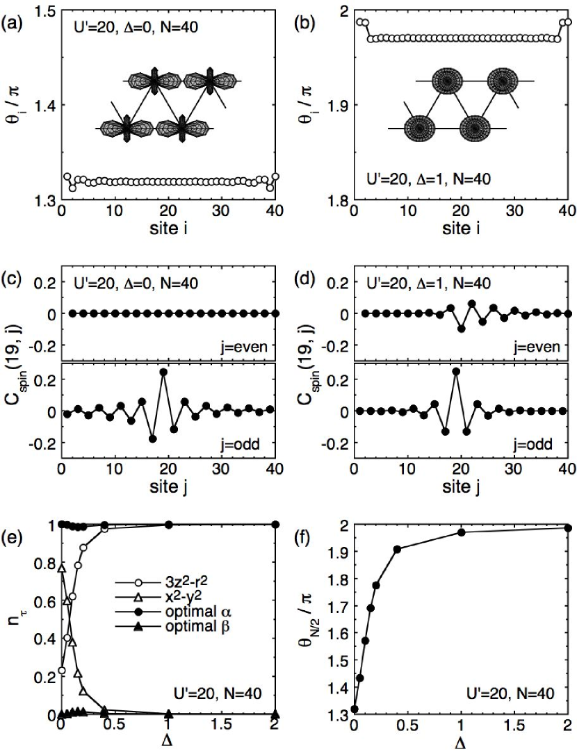
Figure 3: DMRG results for orbital states and spin correlations in the ground state. The site dependence of $\{\theta_{i}\}$ representing orbital arrangement for (a) $\Delta$=0 and (b) $\Delta$=1. Spin correlation function measured from the center site of the lower chain for (c) $\Delta$=0 and (d) $\Delta$=1. (e) Electron densities in $3z^{2}$$-$$r^{2}$, $x^{2}$$-$$y^{2}$, and optimal orbitals as a function of $\Delta$. (f) Angle $\theta_{\bf i}$ at the center site of the system as a function of $\Delta$.

III.1 Spin and orbital structures

Let us first clarify the orbital structure in the spin-singlet ground state, an important issue to understand a key role of orbital anisotropy in geometrically frustrated systems. Irrespective of $\Delta$, we observe that $T({\bf q})$ becomes maximum at ${\bf q}$=0, indicating a FO structure. In Figs. 3(a) and 3(b), we show the optimal set of $\{\theta_{\bf i}\}$ for $\Delta$=0 and 1, respectively. The corresponding orbital arrangement in the bulk is also depicted. At $\Delta$=0, two orbitals are degenerate, but in general, orbital degeneracy is lifted to lower the energy by electron hopping, leading to an optimal path for the electron motion. Indeed, there appears a FO structure characterized by $\theta_{\bf i}$/$\pi$$\sim$1.32, indicating that 3$x^{2}$$-$$r^{2}$ orbital is selectively occupied. The shape of the occupied orbital extends just along the x direction, not along the zigzag path, leading to a double-chain structure for the electron motion. Then, the spin exchange interaction along the zigzag path is expected to be suppressed in comparison with that along the double-chain direction. To clarify this point, we investigate the spin correlation function

$$C_{\rm spin}({\bf i},{\bf j})=\langle S_{\bf i}^{z}S_{\bf j}^{z}\rangle$$ (7)

with $S_{\bf i}^{z}$=$\sum_{\tau}(\rho_{{\bf i}\tau\uparrow}$$-$$\rho_{{\bf i}\tau\downarrow})/2$. In Fig. 3(c), the correlations measured from the center site of the lower chain is shown for $\Delta$=0. We find that there exists an AFM correlation between intrachain sites in each of the double chain, while the spin correlation between the two chains is much weak. Thus, the zigzag chain is decoupled to a double-chain system due to the orbital anisotropy in terms of the spin correlation.

On the other hand, the orbital anisotropy almost disappears at $\Delta$=1, since electrons favorably occupy the lower 3$z^{2}$$-$$r^{2}$ orbital, which is isotropic in the $xy$ plane, as shown in Fig. 3(b). In accordance with the variation of the orbital shape, electrons turn to move along the zigzag path as well as the double-chain direction. Then, the spin correlation appears between the two chains, as shown in Fig. 3(d). Note, however, that orbital degree of freedom is not perfectly quenched due to the level splitting. In fact, it is found that optimal orbitals at the edges deviate from those in the bulk. Namely, the orbital shape in the bulk extends to the double-chain direction in some degree, while it changes to become rather isotropic around the edges so that electrons can smoothly move near the edges. Thus, orbital degree of freedom is still effective, and there occurs the adjustment of the optimal orbital to the environmental lattice inhomogeneity.

In order to gain insight into the change in the orbital state due to the level splitting, we investigate the electron density in each orbital

$$n_{\tau}=\sum_{\bf i}\langle\rho_{{\bf i}\tau}\rangle/N,$$ (8)

as shown in Fig. 3(e). As $\Delta$ is increased, electrons are forced to be accommodated in the lower 3$z^{2}$$-$$r^{2}$ orbital, but the electron density in each of 3$z^{2}$$-$$r^{2}$ and $x^{2}$$-$$y^{2}$ orbitals is found to change gradually without any anomalous behavior. Accordingly, the optimal $\alpha$ orbital state is smoothly transformed from 3$x^{2}$$-$$r^{2}$ to 3$z^{2}$$-$$r^{2}$ with increasing $\Delta$, as shown in Fig. 3(f). On the other hand, we observe that optimal $\alpha$ orbitals are occupied, while $\beta$ orbitals are almost vacant, irrespective of $\Delta$. This behavior is well understood by regarding the level splitting as the fictitious magnetic field in the orbital space. Namely, the direction of fully polarized orbital moment is rotated by the magnetic field. Thus, the present system is always regarded as a one-orbital system composed of optimal $\alpha$ orbitals, although we have considered the multi-orbital system.

III.2 Effective spin model

Let us here consider the effect of the appearance of an orbital arrangement on magnetic properties. For finite $\Delta$, the lower 3$z^{2}$$-$$r^{2}$ orbital is occupied in the atomic limit, but strong electron-electron correlations cause a mixed orbital state of 3$z^{2}$$-$$r^{2}$ and $x^{2}$$-$$y^{2}$ orbitals. In fact, we have found that one optimal orbital becomes relevant due to the FO arrangement, while the relevant orbital is controlled by $\Delta$. In order to understand magnetic properties of such a one-orbital system, it is useful to consider an effective model in the strong-coupling limit. For this purpose, we first express the Hamiltonian in terms of new operators by substituting Eq. (4) as

$${\tilde{H}} = \sum_{{\bf i},{\bf a},\tau,\tau^{\prime},\sigma}\tilde{t}_{\tau\tau^{\prime}}^{{\bf i},{\bf i}+{\bf a}}\tilde{d}_{{\bf i}\tau\sigma}^{{\dagger}}\tilde{d}_{{\bf i}+{\bf a}\tau^{\prime}\sigma}+U\sum_{{\bf i},\tau}\tilde{\rho}_{{\bf i}\tau\uparrow}\tilde{\rho}_{{\bf i}\tau\downarrow}$$ (9)

$$+U^{\prime}\sum_{{\bf i}}\tilde{\rho}_{{\bf i}\alpha}\tilde{\rho}_{{\bf i}\beta}-\Delta\sum_{\bf i}(\cos\theta_{\bf i}{\tilde{T}}_{\bf i}^{z}+\sin\theta_{\bf i}{\tilde{T}}_{\bf i}^{x}),$$

where $\tilde{\rho}_{{\bf i}\tau\sigma}$=${\tilde{d}}_{{\bf i}\tau\sigma}^{{\dagger}}{\tilde{d}}_{{\bf i}\tau\sigma}$, ${\tilde{\rho}}_{{\bf i}\tau}$=$\sum_{\sigma}{\tilde{\rho}}_{{\bf i}\tau\sigma}$, ${\tilde{T}}_{\bf i}^{x}=\sum_{\sigma}(\tilde{d}_{{\bf i}\alpha\sigma}^{{\dagger}}\tilde{d}_{{\bf i}\beta\sigma}+\tilde{d}_{{\bf i}\beta\sigma}^{{\dagger}}\tilde{d}_{{\bf i}\alpha\sigma})/2$, and the summation for the orbital index is taken over optimal $\alpha$ and $\beta$ orbitals in the rotated frame. The hopping amplitude is given by

$$\tilde{t}_{\tau\tau^{\prime}}^{{\bf i},{\bf i}+{\bf a}}=\sum_{\mu,\nu}[R(\theta_{{\bf i}})]_{\tau\mu}t_{\mu\nu}^{\bf a}[R^{-1}(\theta_{{\bf i}+{\bf a}})]_{\nu\tau^{\prime}}.$$ (10)

We note that $U$ and $U^{\prime}$ ($U$=$U^{\prime}$) in Eq. (9) are given by the same ones in the original Hamiltonian Eq. (1), since the orbital basis set is transformed within the rotational invariant orbital space, and thus, the Coulomb integrals are expressed in the same form by Racah parameters. Dagotto2001 Note also that, as mentioned in the previous subsection, the level splitting is regarded as the fictitious magnetic field for the orbital moment $\tilde{T}_{\bf i}^{z}$, while there appears the transverse field for $\tilde{T}_{\bf i}^{x}$.

Magnetic and orbital ordering phenomena in multi-orbital systems have been actively discussed on the basis of an effective spin-orbital model, the so-called Kugel-Khomskii model. Kugel1972 ; Kugel1973 Here, we intend to obtain an understanding of magnetic properties on the orbital-arranged background composed of the relevant $\alpha$ orbital. Thus, we consider a simplified spin model, by ignoring the irrelevant $\beta$ orbital. Then, we keep only the $\alpha$-orbital parts in Eq. (9), such as

$${\tilde{H}}_{\alpha} = \sum_{{\bf i},{\bf a},\sigma}\tilde{t}_{\alpha\alpha}^{{\bf i},{\bf i}+{\bf a}}\tilde{d}_{{\bf i}\alpha\sigma}^{{\dagger}}\tilde{d}_{{\bf i}+{\bf a}\alpha\sigma}+U\sum_{{\bf i}}\tilde{\rho}_{{\bf i}\alpha\uparrow}\tilde{\rho}_{{\bf i}\alpha\downarrow}$$ (11)

$$-(\Delta/2)\sum_{\bf i}\cos\theta_{\bf i}\tilde{\rho}_{{\bf i}\alpha}.$$

Now we apply the second-order perturbation with respect to electron hopping, and reach an effective Heisenberg spin model

$$\tilde{H}_{\rm AFM}=\sum_{{\bf i},{\bf a}}J_{{\bf i},{\bf i}+{\bf a}}({\bf S}_{\bf i}\cdot{\bf S}_{{\bf i}+{\bf a}}-1/4)+E_{\rm s},$$ (12)

where ${\bf S}_{\bf i}$ is a spin-1/2 operator at site ${\bf i}$, the AFM exchange is given by

$$J_{{\bf i},{\bf i}+{\bf a}}=4|\tilde{t}_{\alpha\alpha}^{{\bf i},{\bf i}+{\bf a}}|^{2}/U,$$ (13)

and $E_{\rm s}$ denotes the energy shift due to the level splitting, given by

$$E_{\rm s}=-(\Delta/2)\sum_{\bf i}\cos\theta_{\bf i}.$$ (14)

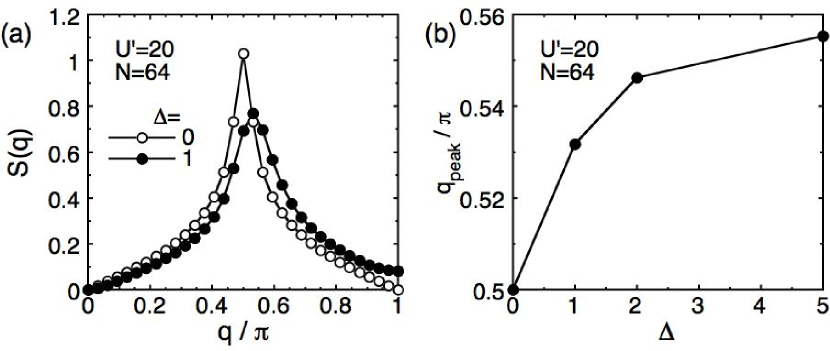
Figure 4: (a) Spin structure factor for $\Delta$=0 and 1 in the ground state. (b) The $\Delta$ dependence of the peak position, estimated from the DMRG results with $N$=64.

It should be noted that this effective model represents a zigzag spin chain including nearest-neighbor exchange $J_{1}$ along the zigzag path and next-nearest-neighbor exchange $J_{2}$ along the double chain. To discuss magnetic properties of the present $e_{\rm g}$-orbital model based on the effective model, let us here summarize the property of the zigzag spin chain, which has been revealed by intensive numerical and analytical investigations. MG1969 ; Haldane1982 ; Tonegawa1987 ; Okamoto1992 ; White1996 In the zigzag spin chain, the ratio of competing exchanges $J_{2}/J_{1}$ is a controlling parameter for the degree of spin frustration. At $J_{2}/J_{1}$=0, the system is equivalent to a single chain, which has a gapless spin-liquid ground state. With the increase of $J_{2}/J_{1}$, the spin frustration becomes effective, and the ground state is changed from a critical spin-liquid phase to a gapped dimer phase at $J_{2}/J_{1}$=0.24. Okamoto1992 The dimer phase continues up to the limit of $J_{2}/J_{1}$=$\infty$, while the spin gap decreases exponentially, White1996 since the system turns to be independent two chains for $J_{2}/J_{1}$=$\infty$. On the other hand, the spin correlation exhibits a commensurate AFM peak at $q$=$\pi$ for 0$<$$J_{2}/J_{1}$$<$1/2, while the peak changes into an incommensurate one for $J_{2}/J_{1}$$>$1/2, and the peak position gradually moves to $q$=$\pi/2$ for infinite $J_{2}/J_{1}$. Tonegawa1987 ; White1996

In order to confirm that magnetic properties are actually described by the zigzag spin chain, let us discuss the behavior of the spin correlation. In Fig. 4(a), we show our DMRG results of the spin structure factor

$$S({\bf q})=\sum_{{\bf i},{\bf j}}\langle S_{\bf i}^{z}S_{\bf j}^{z}\rangle e^{i{\bf q}\cdot({\bf i}-{\bf j})}/N$$ (15)

with $S_{\bf i}^{z}$=$\sum_{\tau}(\rho_{{\bf i}\tau\uparrow}$$-$$\rho_{{\bf i}\tau\downarrow})/2$. Note that the results are depicted with a scalar wavenumber, which is defined by regarding the zigzag path as a linear chain, for comparison with the characteristics of the zigzag spin chain described above. For $\Delta$=0, we clearly observe a peak at $q$=$\pi/2$, consistent with that of the zigzag spin chain with large $J_{2}/J_{1}$, since $J_{2}/J_{1}$=$64^{2}$ for the 3$x^{2}$$-$$r^{2}$ FO arrangement. Note that we evaluate $J_{1}$ and $J_{2}$ at the center of the chain, by ignoring the site dependence in $J_{{\bf i},{\bf i}+{\bf a}}$. The effect of the site dependence of $J_{{\bf i},{\bf i}+{\bf a}}$ on the spin gap will be discussed in the next section. In Fig. 4(b), we show the $\Delta$ dependence of the peak position of the spin structure factor. With increasing $\Delta$, the peak position changes away from $q$=$\pi/2$ towards $q$=$\pi$, as expected by analogy with the zigzag spin chain, since $J_{2}/J_{1}$ approaches unity such as $J_{2}/J_{1}$=1.61 for $\Delta$=1, $J_{2}/J_{1}$=1.24 for $\Delta$=2, and $J_{2}/J_{1}$=1.08 for $\Delta$=5. Note that in the zigzag spin chain, the peak locates at $q$$\sim$$0.561\pi$ for $J_{2}/J_{1}$=1. White1996 In fact, the peak in the present $e_{\rm g}$-orbital model approaches this position with increasing $\Delta$, as shown in Fig. 4(b). Thus, the behavior of the spin structure factor is well understood by analogy with the zigzag spin chain.

IV Spin Excited State

Now we turn our attention to the spin excitation. In order to discuss the spin gap, in general, we consider the lowest-energy state among spin-triplet states. One may expect that such a triplet state is also described by the Heisenberg model, but we should note that the change of the spin state influences on the orbital state as well. Such effect is already found in a two-site problem, as shown in Fig. 5(a). In the upper panel, we depict an AFM/FO configuration in the spin-singlet ground state. On the other hand, in the spin-triplet excited state, an antiferro-orbital configuration turns to be favorable to gain kinetic energy by electron hopping due to the Pauli’s exclusion principle, as shown in the lower panel.

In order to clarify the characteristics of the orbital rotation due to the spin-triplet excitation, we investigate the spin-orbital correlation function, defined by

$$C_{\rm so}({\bf k},{\bf l};{\bf i},{\bf j})=\langle(3/4+{\bf S}_{\bf k}\cdot{\bf S}_{\bf l})T_{\bf i}^{z}T_{\bf j}^{z}\rangle,$$ (16)

which represents the orbital correlation on the condition that the spin state of bond $({\bf k},{\bf l})$ is triplet. In Fig. 5(b), we show the spin-orbital correlation function in the spin-triplet excited state. Here, we set i=k to consider the orbital rotation around the spin-triplet bond. We observe that staggered orbital correlation is enhanced on the spin-triplet bond, as was expected from the two-site problem, while the staggered component rapidly decays for long distances from the spin-triplet bond. Namely, the orbital rotation occurs only close to the spin-triplet bond. Note that orbital correlations near the edges are found to increase due to the deformation of the optimal orbital around the edges, as shown below.

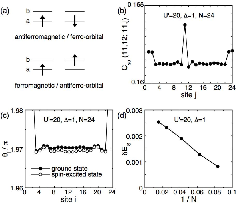
Figure 5: (a) Schematic view of spin-orbital configuration. (b) Spin-orbital correlation function in the spin-excited state. (c) The optimal set of $\{\theta_{\bf i}\}$ in the ground and spin-excited states. (d) The system-size dependence of the difference in the energy shift between ground and spin-excited states.

Since the spin-triplet pair moves in the system with carrying the orbital rotation, it is expected that the averaged orbital structure should be different between the spin-singlet ground state and the spin-triplet excited state. In fact, in the excited state, a FO arrangement is also found to appear and the system is regarded as a one-orbital system in a similar way to the case of the ground state. However, as shown in Fig. 5(c), we clearly observe that optimal orbitals in the excited state are changed from those in the ground state. This behavior is understood from a viewpoint of the adjustment of the optimal orbital. Namely, the orbital state is reorganized so as to provide the most appropriate orbital arrangement for the spin state. Note that in the excited state, the orbital shape around the edges becomes isotropic in comparison with those in the bulk similarly to the case of the ground state.

In order to ascertain this characteristic change of the orbital arrangement, we evaluate the difference in the energy shift,

$$\delta E_{\rm s}=E_{\rm s}^{(1)}-E_{\rm s}^{(0)},$$ (17)

where $E_{\rm s}^{(0)}$ and $E_{\rm s}^{(1)}$ denote the values of $E_{\rm s}$ in the ground and excited states, respectively. In Fig. 5(d), we show the system-size dependence of $\delta E_{\rm s}$. It is observed that $\delta E_{\rm s}$ grows and converges to a finite value with increasing the system size, suggesting that $\delta E_{\rm s}$ will contribute to the spin gap. Concerning exchange interactions $\{J_{{\bf i},{\bf i}+{\bf a}}\}$, we obtain the ratio at the center of the chain as $J_{2}/J_{1}$=1.61 in the ground state, while $J_{2}/J_{1}$=1.62 in the excited state for $\Delta$=1 from the DMRG results of $N$=40. One may consider that the difference seems small, but as we will see later, even such small difference leads to the significant change in the spin gap. In short, the present system can be regarded as a one-orbital system even in the excited state, but the variation of the orbital arrangement appears in the changes of $E_{\rm s}$ and $\{J_{{\bf i},{\bf i}+{\bf a}}\}$ in the effective Heisenberg model. Thus, spin and orbital degrees of freedom dynamically interact with each other, and the spin excitation involves the changes of not only spin state itself, but also orbital state.

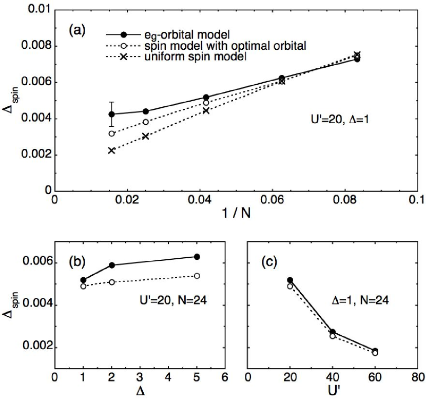
Figure 6: (a) The system-size dependence of spin gap at $\Delta$=1. Errorbars for $N$=40 and 64 are estimated from the truncation error. (b) Spin gap as a function of $\Delta$ for $U^{\prime}$=20 and $N$=24. (c) Spin gap as a function of $U^{\prime}$ for $\Delta$=1 and $N$=24.

Now let us discuss the behavior of the spin gap at $\Delta$=1. From the estimation of $J_{2}/J_{1}$=1.61 in the ground state, the ground state is expected to correspond to the gapped dimer phase of the zigzag spin chain. Tonegawa1987 ; Okamoto1992 ; White1996 To clarify this point, we investigate the system-size dependence of the spin gap

$$\Delta_{\rm spin}=E(N/2+1,N/2-1)-E(N/2,N/2)$$ (18)

up to $N$=64, where $E(N_{\uparrow},N_{\downarrow})$ denotes the lowest energy in the subspace with $N_{\uparrow}$ up- and $N_{\downarrow}$ down-spin electrons. As shown in Fig. 6(a), the spin gap seems to converge to a finite value in the thermodynamic limit. For comparison with the zigzag spin chain, we also evaluate the spin gap for two types of AFM Heisenberg models. First, we take a uniform model, assuming that AFM exchanges are uniformly given by $J_{1}$ and $J_{2}$, which are estimated at the center of the chain for the ground state. In Fig. 6(a), such results are denoted by crosses. Corresponding to the gapped dimer phase, we observe a finite spin gap in the thermodynamic limit, but significant deviation exists between the results of the $e_{\rm g}$-orbital Hubbard model and those of the uniform Heisenberg model.

It is emphasized here that such deviation indicates the effect of the orbital-arranged background which should be different between ground and excited states. Then, we attempt to re-estimate the spin gap by considering the following two points: (i) The optimal orbital is not uniform in the system, especially around the edges, as shown in Fig. 3(b). (ii) The orbital arrangement is found to be different between ground and excited states. To take account of these points, we deal faithfully with the effective Heisenberg model Eq. (12) with the optimal set of $\{\theta_{\bf i}\}$ for both ground and excited states. The variation of $\{J_{{\bf i},{\bf i}+{\bf a}}\}$ causes the change in the energy of the spin system. There also occurs the difference in the energy shift due to the level splitting, as shown in Fig. 5(d). Note that we calculate the spin gap for the model with site-dependent exchange interactions by exploiting the DMRG algorithm for random spin systems. Hida1996 The results are denoted by open circles in Fig. 6(a). We find that the spin gap is appropriately described by the effective Heisenberg model with the optimal orbital rather than the simple uniform Heisenberg model.

Although some deviation still remains, it is improved by increasing $m$ to keep more states in the renormalization step for the $e_{\rm g}$-orbital Hubbard model. Another aspect of the remaining deviation would be the effect of charge and/or orbital fluctuations due to the smallness of the Coulomb interaction to arrive at the strong-coupling limit. We note that larger energy is obtained for the effective Heisenberg model than that for the $e_{\rm g}$-orbital Hubbard model in both ground and excited states, since the fluctuation effects are ignored. However, such increase of the energy is found to be different between ground and excited states. As a result, the spin gap of the effective Heisenberg model becomes small in comparison with the $e_{\rm g}$-orbital Hubbard model. To see the fluctuation effects on the spin gap, we show the $\Delta$ and $U^{\prime}$ dependence of the spin gap in Fig. 6(b) and 6(c), respectively. With increasing $\Delta$, $J_{2}/J_{1}$ approaches unity and the spin gap increases, as expected by analogy with the zigzag spin chain, White1996 while the deviation remains significant due to the effect of charge fluctuation. On the other hand, as shown in Fig. 6(c), the deviation is reduced with increasing $U^{\prime}$, indicating that the spin gap is well reproduced by the effective Heisenberg model with the optimal orbital, when the charge and orbital fluctuations are suppressed. Thus, we conclude that active orbital degree of freedom influences on the spin gap, suggesting that the spin gap should be considered as a spin-orbital gap.

V Summary

In this paper, we have discussed ground-state properties and spin gap of the $e_{\rm g}$-orbital Hubbard model on the zigzag chain. We have found that the system is regarded as an effective spin system on the orbital-arranged background due to the orbital arrangement. At $\Delta$=0, two orbitals are degenerate, but 3$x^{2}$$-$$r^{2}$ orbital is selectively occupied so as to suppress the spin frustration due to the orbital anisotropy. On the other hand, the orbital anisotropy is controlled by $\Delta$. With increasing $\Delta$, the lower 3$z^{2}$$-$$r^{2}$ orbital is favorably occupied and the orbital anisotropy almost disappears, leading to the revival of the spin frustration. Note that the lower 3$z^{2}$$-$$r^{2}$ orbital is also occupied in the atomic limit $U^{\prime}$$\rightarrow$$\infty$ for $\Delta$$>$0. Then, the system is corresponding to the gapped dimer phase of the zigzag spin chain. In actual compounds, $\Delta$ and $U^{\prime}$ could be controlled by hydrostatic or chemical pressure, indicating the control of the degree of the spin frustration and a possible realization of the gapped phase of the zigzag spin chain.

However, orbital degree of freedom is not completely quenched due to the level splitting even at $\Delta$=1. In fact, there appears a spatially non-uniform pattern of the optimal orbital especially around the edges so as to adjust to the lattice inhomogeneity. In addition, the orbital arrangement is flexibly deformed according to the change of the spin state. In order to discuss the spin-gap formation in multi-orbital systems, it is quite important to consider the interplay of spin and orbital degrees of freedom, even when orbital degree of freedom is suppressed due to the level splitting. The spin gap is essentially determined by the spin-orbital coupled excitation. Thus, it is quite natural to consider the spin gap as a spin-orbital gap.

- (1) Proceedings of International Symposium on Quantum Spin Systems, Prog. Theor. Phys. Suppl. 159 (2005).
- (2) M. Hase, I. Terasaki, and K. Uchinokura, Phys. Rev. Lett. 70, 3651 (1993).
- (3) T. Masuda, I. Tsukada, K. Uchinokura, Y. J. Wang, V. Kiryukhin, and R. J. Birgeneau, Phys. Rev. B 61, 4103 (2000).
- (4) H. Fukuyama, T. Tanimoto, and M. Saito, J. Phys. Soc. Jpn. 65, 1182 (1996).
- (5) H. Onishi and S. Miyashita, J. Phys. Soc. Jpn. 69, 2634 (2000).
- (6) A. Oosawa, M. Ishii, and H. Tanaka, J. Phys.: Condens. Matter 11, 265 (1999).
- (7) T. Nikuni, M. Oshikawa, A. Oosawa, and H. Tanaka, Phys. Rev. Lett. 84, 5868 (2000).
- (8) Ch. Rüegg, N. Gavadini, A. Furer, H.-U. Güdel, K. Krämer, H. Mutka, A. Wildes, K. Habicht, and P. Vorderwisch, Nature (London) 423, 62 (2003).
- (9) C. K. Majumdar and D. K. Ghosh, J. Math. Phys. 10, 1388 (1969).
- (10) F. D. M. Haldane, Phys. Rev. B 25, 4925 (1982).
- (11) T. Tonegawa and I. Harada, J. Phys. Soc. Jpn. 56, 2153 (1987).
- (12) K. Okamoto and K. Nomura, Phys. Lett. A 169, 433 (1992).
- (13) S. R. White and I. Affleck, Phys. Rev. B 54, 9862 (1996).
- (14) M. Matsuda and K. Katsumata, J. Magn. Magn. Mater. 140-145, 1671 (1995).
- (15) M. Matsuda, K. Katsumata, K. M. Kojima, M. Larkin, G. M. Luke, J. Merrin, B. Nachumi, Y. J. Uemura, H. Eisaki, N. Motoyama, S. Uchida, and G. Shirane, Phys. Rev. B 55, R11953 (1997).
- (16) H. Kikuchi, H. Nagasawa, Y. Ajiro, T. Asano, and T. Goto, Physica B 284-288, 1631 (2000).
- (17) M. Hagiwara, Y. Narumi, K. Kindo, N. Maeshima, K. Okunishi, T. Sakai, and M. Takahashi, Physica B 294-295, 83 (2001).
- (18) N. Maeshima, M. Hagiwara, Y. Narumi, K. Kindo, T. C. Kobayashi, and K. Okunishi, J. Phys. Condens. Matter 15, 3607 (2003).
- (19) H. Onishi and T. Hotta, Physica B 359-361, 669 (2005).
- (20) H. Onishi and T. Hotta, Phys. Rev. B 71, 180410(R) (2005).
- (21) H. Onishi and T. Hotta, Physica B 378-380, 589 (2006).
- (22) J. van den Brink, W. Stekelenburg, D. I. Khomskii, and G. A. Sawatzky, Phys. Rev. B 58, 10276 (1998).
- (23) J. Bala, A. M. Oleś, and G. A. Sawatzky, Phys. Rev. B 63, 134410 (2001).
- (24) J. C. Slater and G. F. Koster, Phys. Rev. 94, 1498 (1954).
- (25) See, for instance, T. Hotta, Rep. Prog. Phys. 69, 2061 (2006).
- (26) E. Dagotto, T. Hotta, and A. Moreo, Phys. Rep. 344, 1 (2001).
- (27) S. R. White, Phys. Rev. Lett. 69, 2863 (1992).
- (28) For review, see U. Schollwöck, Rev. Mod. Phys. 77, 259 (2005).
- (29) T. Hotta, Y. Takada, and H. Koizumi, Int. J. Mod. Phys. B 12, 3437 (1998).
- (30) K. I. Kugel and D. I. Khomskii, Sov. Phys. JETP Lett. 15, 446 (1972).
- (31) K. I. Kugel and D. I. Khomskii, Sov. Phys. JETP 37, 725 (1973).
- (32) Another type of complex orbital ordering has been discussed for manganites. R. Maezono and N. Nagaosa, Phys. Rev. B 62, 11576 (2000); J. van den Brink and D. Khomskii, Phys. Rev. B 63, 140416 (2001); K. Kubo and D. S. Hirashima, J. Phys. Soc. Jpn. 71, 183 (2002).
- (33) T. Hotta, A. L. Malvezzi, and E. Dagotto, Phys. Rev. B 62, 9432 (2000).
- (34) K. Hida, J. Phys. Soc. Jpn. 65, 895 (1996).