Spacetime thermodynamics and subsystem observables in a kinetically constrained model of glassy materials

Abstract

In a recent article [M. Merolle et al., Proc. Natl. Acad. Sci. USA 102, 10837 (2005)], it was argued that dynamic heterogeneity in $d$-dimensional glass formers is a manifestation of an order-disorder phenomenon in the $d+1$ dimensions of space-time. By considering a dynamical analogue of the free energy, evidence was found for phase coexistence between active and inactive regions of space-time, and it was suggested that this phenomenon underlies the glass transition. Here we develop these ideas further by investigating in detail the one-dimensional Fredrickson-Andersen (FA) model in which the active and inactive phases originate in the reducibility of the dynamics. We illustrate the phase coexistence by considering the distributions of mesoscopic space-time observables. We show how the analogy with phase coexistence can be strengthened by breaking microscopic reversibility in the FA model, leading to a non-equilibrium theory in the directed percolation universality class.

I Introduction

Figure 1: Illustration of a trajectory in a facilitated model with space-time “bubbles” of the inactive state. The boxes illustrate finite observation space-time windows: the top one corresponds to a typical region; the bottom one is a rare collective fluctuation of size much larger than those typical of the active state. On the right are trajectories from the one-spin facilitated one-dimensional Fredrickson-Andersen model Fredrickson and Andersen (1984), at $T=1$ for observation windows of $L=180$ and $t_{\rm obs}=320$ (smaller observation windows of $L=60$ are also outlined).

The hallmarks of the glass transition Rev (a) are a sudden increase of relaxation times, and dynamic heterogeneity Rev (b). A recent paper Merolle et al. (2005) described the idea that these phenomena are manifestations of phase coexistence in space-time. The two competing phases are an active state, containing many relaxation events, and an inactive one, where these events are scarce. The purpose of the current paper is to develop these ideas by building on the results of Ref. Merolle et al. (2005).

In the active phase of the dynamics, the existence of the inactive phase can be inferred by measuring the distribution of any observable that measures the quantity of relaxation events within a finite space-time window Merolle et al. (2005). Because of the coexisting inactive phase, these distributions display non-Gaussian tails. This behaviour is analogous to the situation in standard phase transitions: the distribution of cavity sizes in a fluid near liquid vapour coexistence has non-Gaussian tails Huang and Chandler (2000), as does the distribution of box magnetization for the Ising model in the vicinity of its phase transition Clusel et al. (2004).

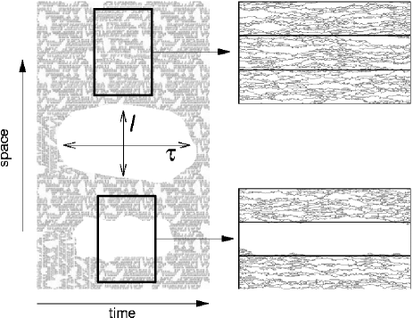
The concept of space-time thermodynamics that we use Merolle et al. (2005) is illustrated in Fig. 1. It employs a simple picture of glassy dynamics at low temperatures, in which diffusing excitations coalesce and branch Garrahan and Chandler (2002). This dynamics is reducible Ritort and Sollich (2003). That is, there are two steady states, an active one with a finite density of excitations, and an inactive one with strictly zero density. Working in the active state, the dominant fluctuations on large length scales are space-time regions in which there are no excitations, as illustrated in Fig. 1. We refer to these regions as “bubbles” of the inactive phase.

We characterise the bubbles by the probability density function $P_{\mathrm{bubble}}(l,\tau)$ for their spatial and temporal extents (denoted $l$ and $\tau$, respectively). To the extent that these rare fluctuations are dynamical analogues of those near phase coexistence, and for bubbles which are large compared with the bulk correlation length of the active state, we can write:

$$P_{\mathrm{bubble}}(l,\tau)\propto\exp\left\{-\left[\sigma_{1}l+\sigma_{2}\tau+\mu l\tau+\Lambda(l-v\tau)^{2}\right]\right\},$$ (1)

where $\sigma_{1}$ and $\sigma_{2}$ are, in effect, surface tensions in the spatial and temporal directions respectively, $\mu$ is the difference between the bulk free energy densities of active and inactive phases, and $\Lambda$ controls the aspect ratio of the bubbles, in conjunction with the velocity parameter $v$. This distribution of (1) can be investigated by considering the probability distribution functions for observables that are averaged over finite regions of space-time, such as the boxes in Fig. 1 Merolle et al. (2005). Large rare bubbles dominate the tails of these distributions.

The terminology “free energy”, as used in the previous paragraph, refers to space-time; the relevant ensemble is a the space of histories (or trajectories) of the system, which is observed for a specified period of time, $t_{\mathrm{obs}}$. This concept of a free energy is central to Ref. Merolle et al. (2005), and it is found also in the thermodynamic formulation of dynamics due to Ruelle RuelleBook ; Lecomte06 . In particular, for a $d$-dimensional system, one considers statistical mechanics in the corresponding $(d+1)$-dimensional space. The extra dimension is that of time, so the resulting space is necessarily anisotropic.

Thus, to appreciate the analogy with phase coexistence for $d=1$, consider an anisotropic two-dimensional Ising model below its critical temperature, with a small field stabilising the spin-up phase. The spins are predominately up, but there will be a distribution of spin-down domains with various sizes. In the case where the interactions are different in the $x$ and $y$ directions, the distribution of sizes for domains of the spin-down phase is of the form

$$P_{\mathrm{down}}(x,y)\propto\exp\left\{-\left[\sigma_{x}x+\sigma_{y}y+\mu^{\prime}xy+\Lambda^{\prime}(x-v^{\prime}y)^{2}\right]\right\},$$ (2)

where $x$ and $y$ are the extents of the bubbles in the $x$ and $y$ directions; $\sigma_{x}$ and $\sigma_{y}$ are surface tensions; $\mu^{\prime}$ is the free energy difference between up and down phases (proportional to the small field); and $\Lambda^{\prime}$ and $v^{\prime}$ set the shape of the bubbles.

Figure 2: Sketch illustrating the effect of the choice of initial condition in a model of diffusing excitations that branch and coalesce. An initial state with no excitations (left) persists throughout the observation time. All other initial conditions result in the system exploring the active steady state (right).

As phase coexistence is approached in the Ising system, the free energy difference $\mu^{\prime}$ approaches zero. In the dynamical system, the corresponding limit is $\mu\to 0$, in which case active and inactive states coexist. A central result of this article is that $\mu=0$ for systems in which the dynamics is reducible into active and inactive partitions. Within the thermodynamic formalism of Ruelle the free energy difference $\mu$ is the difference in the so-called ‘topological pressure’ RuelleBook ; Lecomte06 between the active and inactive phases of the dynamics.

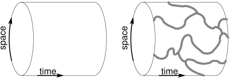
Since the phases are at coexistence in these models, a boundary condition suffices to make the system choose one phase. For example, consider a system with periodic spatial boundary conditions, as sketched in Fig. 2. If we choose our initial condition to be completely inactive, then this state persists forever; all other initial conditions lead to the active state.

In this article, we use the the Fredrickson-Andersen (FA) facilitated spin model Fredrickson and Andersen (1984) as an illustrative system. In the following section, we probe the distribution of (1) by analysing the distributions of space-time observables, such as the total amount of dynamical activity inside a given spatial region, integrated over a finite observation time. The forms of these distributions also imply that $\mu=0$, in accordance with our analytic arguments.

We also compare the FA model with two other systems. In Ref. Jack et al. (2006), a model with appearing and annihilating excitations (the so-called AA model) was shown to have the same two point correlations as the FA model (up to a multiplicative factor). However, we show that this model has mesoscopic fluctuations that are very different from those of the FA model. Conversely, breaking microscopic reversibility in the FA model moves moves the system into the directed percolation (DP) universality class Hinrichsen (2000). In that case, the the two point functions and critical scaling change qualitatively. However, the active and inactive states still coexist, so the fluctuations are still well-described by the phase coexistence analogy.

The paper is organized as follows. In section II we define the model, discuss its trajectories, and introduce the observables of interest. We also show that reducibility of the dynamics is essential to see the phase coexistence effect. In section III we formalise our discussion of space-time thermodynamics by considering the distribution of the dynamical action that is analogous to the thermodynamic free energy. We consider the effect of breaking microscopic reversibility in section IV.

II Models, trajectories and observables

Kinetically constrained models (see Ref. Ritort and Sollich (2003) for a comprehensive review) are defined in such a way that their non-trivial behaviour is purely dynamical in origin. Thus, they are the natural framework for investigating dynamical heterogeneity and its consequences Harrowell (1993); Garrahan and Chandler (2002, 2003); Jung et al. (2004); Toninelli et al. (2005); Bertin et al. (2005).

A very simple kinetically constrained model is the single-spin facilitated FA model Fredrickson and Andersen (1984); Ritort and Sollich (2003) in dimension $d=1$. It is defined for a chain of $N$ binary variables $n_{i}\in\{0,1\}$, with trivial Hamiltonian $H=J\sum_{i}n_{i}$. The model evolves under the following Monte-Carlo (MC) dynamics. At each MC iteration a randomly chosen site $i$ changes state according to:

$$n_{i}=0 \rightarrow n_{i}=1\qquad\hbox{probability }f_{i}e^{-\beta},$$

$$n_{i}=1 \rightarrow n_{i}=0\qquad\hbox{probability }f_{i},$$

where we have set $J=1$ and $\beta\equiv T^{-1}$. The non-trivial part of the dynamics is due to the facilitation function

$$f_{i}\equiv n_{i+1}+n_{i-1}-n_{i+1}n_{i-1}.$$ (3)

That is, a spin flip on site $i$ can take place only if at least one if its nearest neighbours is in the excited state. Since $f_{i}$ does not depend on $n_{i}$ then the time evolution of the model obeys detailed balance with respect to $H$ at temperature $\beta^{-1}$. The mean density of up spins in the active state is

$$c\equiv(1+e^{\beta})^{-1}.$$ (4)

The unit of time is an MC sweep ($N$ attempted spin flips).

In the following, we consider an FA model in which $N$ is to be taken to infinity in the thermodynamic limit. We will take a subsystem of this model, containing $L+2$ spins, $\{n_{0},\dots,n_{L+1}\}$. The length $L$ is to remain finite: it is a mesoscopic quantity. A trajectory for the subsystem specifies the state of the $(L+2)$ spins at $Nt_{\mathrm{obs}}$ MC steps. The trajectory is defined within a space-time observation box of size $Lt_{\rm obs}$. We consider observables such as the density of excitations within the box, for a given trajectory:

$$m_{\mathrm{traj}}=(LNt_{\rm obs})^{-1}\sum_{i=1}^{L}\sum_{\tau=1}^{Nt_{\rm obs}}n_{i,\tau},$$ (5)

where $n_{i\tau}$ is the state of the $i$th spin in the $\tau$th state of the trajectory. Note that the boundaries $n_{0}$ and $n_{L+1}$ do not appear in the sum.

The quantity $m_{\mathrm{traj}}$ is analogous to the net magnetization of a $(d+1)$-dimensional Ising model, and thus we often refer to it as the “magnetization”. However, its physical meaning is that of mobility or activity, i.e., the net number of cells in the observed space-time volume that exhibit an appreciable degree of molecular motion. This meaning is that of Garrahan and Chandler’s coarse grained view of structural glasses Garrahan and Chandler (2002, 2003). In an atomistic treatment, a corresponding quantity can be expressed in terms of the observable $\hat{F}_{j}(\bm{k},\delta t,t)=\cos\{\bm{k}\cdot[\hat{\bm{r}}_{j}(t+\delta t)-\hat{\bm{r}}_{j}(t)]\}$ where $\hat{\bm{r}}_{j}(t)$ is the position of the $j$th particle at time $t$, and $\bm{k}$ is a microscopic wave vector (on the order of the inverse particle size). If $\hat{F}_{j}(\bm{k},\delta t,t)$ is small, then particle $j$ experienced a relaxation event between times $t$ and $t+\delta t$. For a subsystem of particles, $S$, we define the density of relaxation events, or net mobility, in space and time to be

$$\hat{K}_{\mathrm{traj}}(\bm{k},\delta t)=(t_{\mathrm{obs}}N_{S})^{-1}\sum_{j\in S}\int_{0}^{t_{\mathrm{obs}}}\!\mathrm{d}t\,[1-\hat{F}_{j}(\bm{k},\delta t,t)]$$ (6)

where $N_{S}$ is the number of particles in the subsystem $S$. The quantity $\hat{K}_{\mathrm{traj}}(\bm{k},\delta t)$ is parametrised by microscopic length and time scales ($|\bm{k}|^{-1}$ and $\delta t$), and is summed over a mesoscopic region of space-time. The parameters $|\bm{k}|^{-1}$ and $\delta t$ coincide with coarse graining lengths and time, respectively.

The fluctuations in $\hat{K}_{\mathrm{traj}}(\bm{k},\delta t)$ are related to four point observables Toninelli et al. (2005); the distribution of $\hat{K}_{\mathrm{traj}}(\bm{k},\delta t)$ is also related to the distributions of correlation functions measured in Cipelletti05 ; Chamon04 . Results for distributions of the density of relaxation events in atomistic glass-formers show non-Gaussian tails similar to those that we present here Lutz_kinks . However, the purpose of this article is to discuss generic properties of dynamically heterogeneous systems, so we restrict ourselves to very simple models.

II.1 Distribution of the event densities

We consider the distribution of the trajectory activity, or box magnetisation $m_{\mathrm{traj}}$:

$$P(m)=\sum_{\mathrm{traj}}P_{\mathrm{traj}}\delta(m-m_{\mathrm{traj}}).$$ (7)

The sum is over all possible trajectories of the system, with their associated probabilities $P_{\mathrm{traj}}$. In the limit of $L\to\infty$ or $t_{\rm obs}\to\infty$, the central limit theorem states that $P(m)$ will be sharply peaked around $m=c$, with a variance that scales as $(Lt_{\rm obs})^{-1}$. The observation of Ref. Merolle et al. (2005) was that while this is the case in the limit of large $(Lt_{\rm obs})$, the distribution of $m$ remains non-trivial even for $L\gg\xi$ and $t_{\rm obs}\gg\tau$, where $\xi\approx c^{-1}$ and $\tau\approx c^{-3}$ are the correlation length and time associated with the zero temperature dynamical fixed point of this model.

Figure 3: Distribution of trajectory magnetization $P(m)$ at $\beta=1$, $L=60$ and various observation times. We use $N=180$ which is large enough so that $P(m)$ does not depend on $N$. The exponential tails of $P(m)$ all have similar gradients: the dotted lines are $P(m)\propto\exp(\sigma m)$ with $\sigma=87$.

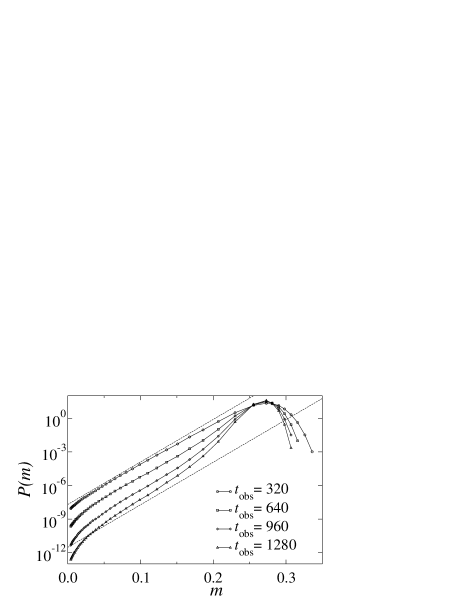
We show various $P(m)$ in Fig. 3. The peak of $P(m)$ is Gaussian, and this corresponds to trajectories like the one on the top-right of Fig. 1. The tails of $P(m)$ are exponential for small $m$. This data was obtained using a combination of transition path sampling (TPS) Bolhuis et al. (2002) and umbrella sampling Frenkel and Smit (2001). For details see the Appendix. The trajectories in the tail are dominated by rare large regions which have no excitations, like the the one on the bottom-right of Fig. 1.

To explain the presence of the exponential tail, suppose that we have a trajectory with an initial condition containing a large empty region of size $x$, and that this empty region persists throughout $t_{\rm obs}$, leading to a box magnetisation that is small. Now consider a trajectory whose initial condition has an empty region of size $x+(\Delta x)$, but is otherwise identical to the original one. Then the probabilities of the two trajectories are in the ratio $(1-c)^{\Delta x}$, and their magnetisations differ by approximately $c(\Delta x)/L$. Thus we predict

$$P(m)\sim(1-c)^{mL/c}=\exp[(mL/c)\ln(1-c)].$$ (8)

The significance of this result is that the right hand side is independent of $t_{\rm obs}$: increasing the observation time changes the factor multiplying the tail in $P(m)$, but the gradient of the tail remains constant. Fig.  3 shows that the gradient is indeed independent of $t_{\rm obs}$. However, the quantitative prediction for its value is accurate only to within 20-30%. This inaccuracy arises because the large inactive region may extend beyond the edge of the box. Thus, adding extra down sites to the initial condition may decrease the magnetisation by an amount less than $(c/L)$.

Figure 4: We show $P(m)$ at $\beta=1$ for varying $L$ and $t_{\rm obs}$. We use $N=\max(120,3L)$ which is large enough that the results do not depend on $N$. (Top) Increasing observation time at at fixed $L=20$. (Middle) Increasing box size $L$ at $t_{\rm obs}=320$. As $L$ or $t_{\rm obs}$ is increased, we move from a regime in which the tail gradient is independent of the increasing parameter to a regime in which the gradient is proportional to that parameter. (Bottom) We show a typical trajectory for large $t_{\mathrm{obs}}$ and $L=20$ where the observation box is outlined: the size of the total spatial region shown is $N=60$. For large $L$ the trajectories are of the form shown in Fig. 1.

In Fig. 3, the exponential tail of $P(m)$ depends only on $L$ and not on $t_{\rm obs}$, but this is a result of the shape of the observation box: the behaviour of $P(m)$ is symmetric with respect to $L$ and $t_{\rm obs}$. In Fig. 4 we show how $P(m)$ changes as we change the aspect ratio of the observation box. There is a crossover at $L\sim vt_{\rm obs}$, where $v\simeq 0.06$ at $\beta=1$. For $L>vt_{\rm obs}$ the gradient of the exponential tail is independent of $t_{\rm obs}$ as described above, but for $L<vt_{\rm obs}$ then the argument must be modified. Typical trajectories at small $m$ change their form to that shown in Fig. 4 (right). In that case, increasing the width of the bubble does not change $m$; we must instead increase the time for which the inactive state persists. Repeating the argument leads to a situation in which the gradient of the exponential tail is proportional to $t_{\rm obs}$ and independent of $L$, see Fig. 4. In other words, the gradient of the exponential tail is proportional to $\max(L,vt_{\rm obs})$. The spatial and temporal extent of the box enter on equal footing. The data of Fig. 4 is consistent with the crossover from large $L$ to large $t_{\rm obs}$ occuring when $t_{\rm obs}$ is of the order of the first passage time across a bubble of size $L$. This time scales as $(L/v)\sim(L/c^{2})$ since the spreading velocity Hinrichsen (2000) in the FA model is $v\sim(\xi/\tau)\sim c^{2}$.

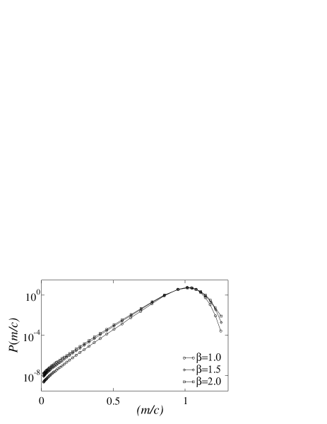
Consistent with the known scaling of the FA model in one dimension Ritort and Sollich (2003), we find that the temperature dependent of $P(m)$ can be accounted for by using rescaled variables. The function

$$P(m/c;cL,c^{3}t_{\rm obs})$$ (9)

depends only weakly on $c$, as shown in Fig. 5. While subleading corrections to the scaling do appear to be significant, there is no qualitative change on lowering the temperature. This justifies our working at inverse temperatures around $\beta=1$, where the data is easier to obtain than in the more glassy regime of the FA model ($\beta>1$).

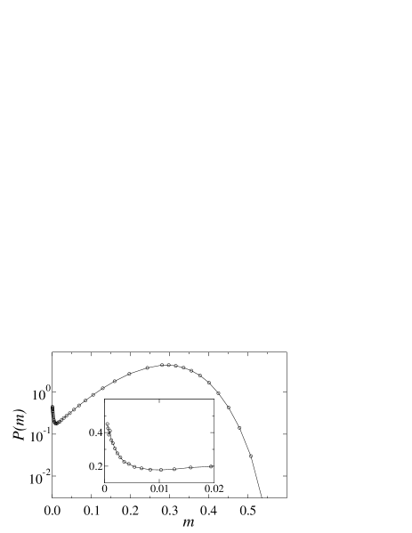
As a final observation in this subsection, we note that the behaviour of $P(m)$ for small observation boxes, $cL<1$ or $c^{3}t_{\rm obs}<1$, is different from that for large boxes. This is shown in Fig. 6. The distribution acquires a secondary peak at $m\to 0$: there is a finite probability of observing $m=0$, so that $P(m)$ diverges as $m\to 0$. We will return to this feature below.

II.2 Comparison with a model of appearing and annihilating excitations (AA model)

In the previous subsection, the non-trivial structure in $P(m)$ occurs in the tails of the distribution. It is associated with rare collective fluctuations in the system. We will argue below that these rare fluctuations do contain significant information about the model. We first compare the magnetisation distributions of the FA model and the AA model of Jack et al. (2006). The AA model has the same two-point correlation functions as the FA model in equilibrium, but other properties of the two systems are qualitatively different.

We define the AA model by specifying local moves for a chain of binary variables:

$$(n_{i},n_{i+1})=(1,0) \leftrightarrow (n_{i},n_{i+1})=(0,1),\qquad\hbox{rate }\gamma e^{-\beta^{\prime}}$$

$$(n_{i},n_{i+1})=(1,1) \rightarrow (n_{i},n_{i+1})=(0,0),\qquad\hbox{rate }\gamma$$

$$(n_{i},n_{i+1})=(0,0) \rightarrow (n_{i},n_{i+1})=(1,1),\qquad\hbox{rate }\gamma e^{-2\beta^{\prime}}$$

where $\gamma=2/(1-e^{-\beta^{\prime}})^{2}$ is an arbitrary temperature dependent factor that rescales the time, chosen for later convenience. These rates again respect detailed balance with respect to $H=\sum_{i}n_{i}$, and the inverse temperature is $\beta^{\prime}$.

Correlation functions in the steady state of the AA model at a given temperature are related to those in the FA model at a different temperature Jack et al. (2006) (strictly this holds when the facilitation function is proportional to the number of up neighbours, not when it is equal to zero or one as here, but there is no qualitative change to the physics). The relationship between correlators depends only on simple multiplicative factors, for example Jack et al. (2006)

$$\langle n_{it}n_{jt^{\prime}}\rangle_{\mathrm{FA},\beta}-\langle n\rangle_{\mathrm{FA,\beta}}^{2}=$$ (10)

$$\frac{4}{1+e^{-\beta}}\left(\langle n_{it}n_{jt^{\prime}}\rangle_{\mathrm{AA},\beta^{\prime}}-\langle n\rangle_{\mathrm{AA,\beta^{\prime}}}^{2}\right),$$

where $\beta$ is the inverse temperature in the FA model and $\beta^{\prime}$ the inverse temperature in the AA model. Equation (10) holds when

$$e^{-\beta^{\prime}}=\frac{\sqrt{1+e^{-\beta}}-1}{\sqrt{1+e^{-\beta}}+1}.$$ (11)

Figure 5: Data showing (approximate) scaling of $P(m)$ in the FA model at various temperatures, scaled according to (9). We plot $P(m/c)$: the box sizes are $L=(60,88,135)$; the observation times are $t_{\rm obs}=(320,1280,5330)$; and we use $N=3L$. These temperatures are not very small, so there are subleading corrections to scaling, but there is no qualitative change to the scaled distribution on lowering the temperature. Further, the computational time required at $\beta=2$ is quite significant, so we cannot rule out small systematic errors arising from non-convergence of our TPS procedure (see appendix).

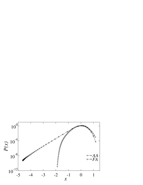
It is clear from (10) that the scaling behaviour and critical properties of the FA and AA models are the same. However, their activity or magnetisation distributions are different, as shown in Fig. 7. The exponential tail is absent in the AA case. Moreover, the persistence functions of the two models are different [the persistence function is the probability that a site does not flip at all in an interval of length $t$]. The fluctuations responsible for the tails in $P(m)$ can be linked to the decoupling of exchange and persistence times in the FA model Jung et al. (2005), a feature which is absent in the AA case. We argue that there are important differences between the dynamics of the FA and AA models: subsystem observables like $P(m)$ make these differences clear where two-point functions like $\langle n_{i\tau}n_{j0}\rangle$ do not.

Figure 6: Plot of $P(m)$ at $\beta=1$, $L=2$, $t_{\rm obs}=160$, showing secondary maximum at small $m$. (Inset) Enlargement of the secondary peak, shown in a linear scale for $P(m)$.

III Dynamical action and thermodynamic analogy

We have shown that the distribution of subsystem magnetisations in the FA model has an exponential tail at small magnetisation. We also showed that this tail comes from rare mesoscopic regions of space-time in which there are no relaxation events. In this section we study the statistical mechanics of the space-time configurations of the subsystem. We draw an analogy between these space-time statistics and the thermodynamic statistics of a system near a phase coexistence boundary.

Figure 7: Distribution of (reduced) box magnetization in the FA and AA models. The reduced variable $x=(m-\langle m\rangle)/\sigma_{m}$ where $\sigma_{m}^{2}\equiv\langle(m-\langle m\rangle)^{2}\rangle=c(1-c)L^{-1}$ is the variance of the instantaneous magnetisation. Parameters are $L=60$, $t_{\rm obs}=320$, $N=180$; in the FA model $\beta=1$; in the AA model $\beta^{\prime}$ is given by (11) with $\beta=1$. For the AA model, $P(m)$ is close to Gaussian. The standard deviation $\sigma_{m}$ is not trivially related to the variance of the box magnetisation, so the fact that the Gaussian parts of the two distributions are very similar is a non-trivial consequence of the exact mapping between the two models.

III.1 Thermodynamic analogy

To make this analogy concrete, we define the probability of a trajectory being generated by some (Markovian) dynamical rules:

$$P_{\mathrm{traj}} = \prod_{\tau=1}^{Nt_{\rm obs}-1}W(s_{\tau+1}|\{s_{\tau},n_{0,\tau},n_{L+1,\tau}\})$$ (12)

$$\times P_{0}(s_{1})P_{\mathrm{bc}}(n_{0,t},n_{L+1,t}),$$

where $s_{\tau}=\{n_{1\tau},\dots,n_{L\tau}\}$ represents the state of the system at time $\tau$; the transition probabilities are denoted by $W(s^{\prime}|\{s,n_{0},n_{L+1}\})$; $P_{\mathrm{bc}}(n_{0,t},n_{L+1,t})$ is the probability of the trajectory of the two boundary spins; and $P_{0}(s_{1})$ is the probability of the initial condition ($s_{1}$). We note that the transition probabilities into a state $s_{\tau+1}$ depend on the state of the boundary spins as well as the state $s_{\tau}$.

It is convenient to define the dynamical action,

$$\mathcal{E}_{\mathrm{traj}}=-\ln P_{\mathrm{traj}},$$ (13)

and the dynamical partition sum,

$$\mathcal{Z}_{b}=\sum_{\mathrm{traj}}e^{-b\mathcal{E}_{\mathrm{traj}}}$$ (14)

which is equal to unity when $b=1$. The extensivity properties of the action $\mathcal{E}$ will be discussed below. To make the correspondence with a thermodynamic partition sum, we simply define

$$Z=\sum_{\mathrm{conf}}e^{-\beta U_{\mathrm{conf}}},$$ (15)

where the sum is over configurations of a system; $U_{\mathrm{conf}}$ is the energy of a configuration; and $\beta$ is the inverse temperature. The application of thermodynamic formalism to dynamical objects such as $\mathcal{Z}_{b}$ is found in the work of Ruelle RuelleBook . A very recent and detailed discussion of its application to Markov chains is given in Lecomte06 ; the parameter $s$ of that paper is $1-b$ in our notation; the Kolmogorov-Sinai entropy $h_{\mathrm{KS}}$ of the Ruelle formalism is the mean action, $\langle\mathcal{E}\rangle$ in our notation.

To treat phase coexistence in ordinary thermodynamics, one may decompose the partition function into its pure states ParisiStatMech

$$Z=\sum_{\alpha}Z_{\alpha}$$ (16)

where $Z_{\alpha}$ is the contribution of pure state $\alpha$ to the partition sum. For example, in the Ising system then the two pure states have positive and negative magnetisations, and statistical weights $Z_{\uparrow}$ and $Z_{\downarrow}$. The difference in free energy density between the two states is

$$\mu^{\prime}=\lim_{N\to\infty}N^{-1}\log(Z_{\uparrow}/Z_{\downarrow}).$$ (17)

At phase coexistence, we have $\mu^{\prime}=0$. The result is that subextensive contributions to $\log(Z_{\uparrow}/Z_{\downarrow})$ from boundary conditions are sufficient to select one phase over the other.

By analogy, for dynamically heterogeneous systems, we make an decomposition of $\mathcal{Z}$ into its reducible partitions Ritort and Sollich (2003). If there are two such partitions then we write

$$\mathcal{Z}_{b=1}=P_{\mathrm{ic}}(1)+P_{\mathrm{ic}}(2)$$ (18)

where the two terms are the probabilities that an initial condition lies in one partition or the other. We then define

$$\mu=\lim_{N,t_{\mathrm{obs}}\to\infty}(Nt_{\mathrm{obs}})^{-1}\log[P_{\mathrm{ic}}(1)/P_{\mathrm{ic}}(2)],$$ (19)

by analogy with the static free energy difference $\mu^{\prime}$.

The probabilities $P_{\mathrm{ic}}(1)$ and $P_{\mathrm{ic}}(2)$ are independent of $t_{\mathrm{obs}}$, so $\mu$ vanishes as $t_{\mathrm{obs}}$ is taken to $\infty$, and an initial condition on the system is sufficient to select the active or inactive partition of the dynamics: see figure 2. In a similar way, a boundary condition is sufficient to select the up or down pure state in an Ising system below the critical temperature. Recalling (1) and (2), we observe that phase coexistence and reducibility lead to distributions with $\mu^{\prime}=0$ and $\mu=0$ respectively. The free energy cost associated with large bubbles (or down domains) comes from their boundaries and not from the bulk.

III.2 Discussion of magnetisation distributions

Fig. 1 illustrates how FA model trajectories with low densities of relaxation events typically contain a large compact “bubble” in which there are no relaxation events. In the FA model then these large bubbles are more common than homogeneous reductions in the density. Conversely, in the AA model, the large bubbles are absent and the homogeneous regions of low density determine the tail of the magnetisation distribution (recall figure 7).

The FA model is reducible, so the distribution of large bubbles will be that of (1), with $\mu=0$ [recall (19)]. The derivation of the magnetisation distribution from the bubble distribution depends on the ratio of $L$ and $t_{\mathrm{obs}}$. For observation windows such that $vt_{\rm obs}<L$, trajectories with small $m_{\mathrm{traj}}$ contain large bubbles that span the temporal extent of the observation window, as in the lower right panel of figure 1. In that case, we have

$$m\simeq c[1-(l/L)].$$ (20)

where $l$ is the spatial extent of the bubble. The probability of the box containing a bubble of this size and shape is

$$P(l)\simeq\int_{t_{\rm obs}}^{\infty}\!\!\!\mathrm{d}\tau\,P(l,\tau).$$ (21)

Assuming that $\Lambda$ is not too small, so that $P(l,\tau)$ is sharply peaked around $l=v\tau$, then

$$\frac{\mathrm{d}}{\mathrm{d}m}\ln P(m)\simeq(L/c)\left[\sigma_{1}+(\sigma_{2}/v)+2(\mu/v)L(1-m/c)\right],$$ (22)

for $m<c[1-(vt_{\rm obs}/L)]$. Unless $\mu$ is very small, the term proportional to $\mu$ will dominate at large $L$, leading to a Gaussian distribution. However, in the case of small $\mu$, the distribution is exponential in $m$, and the gradient of this exponential tail is proportional to $L$ and independent of $t_{\rm obs}$, as observed in Fig. 3. A similar argument holds in the opposite regime of $L<vt_{\rm obs}$ and $m<c[1-(L/vt_{\rm obs})]$, which explains the exponential tails of Fig. 4.

Pursuing the analogy with phase coexistence, we identify the active partition of the dynamics with a dense phase and the inactive partition with a sparse phase. The density of dynamical activity in the active phase is $\langle m\rangle=c$. The typical length scale associated with bubbles of the sparse phase is $\sigma_{1}^{-1}$ which scales as $c^{-1}$. Thus, the typical bubble size and the typical spacing between excitations scale in the same way as the temperature is reduced. This scaling Jack et al. (2006) is consequence of detailed balance in the FA model, which implies that excitations are uncorrelated at equal times: $\langle(n_{i\tau}-c)(n_{j\tau}-c)\rangle=c(1-c)\delta_{ij}$.

In section IV, we will show how generalising the FA model to a system which does not obey detailed balance leads to a situation in which the typical bubble sizes are larger than the excitation spacing. This situation is the usual one in systems at phase coexistence: the FA model is a special case because of the extra symmetry of detailed balance.

III.3 Distribution of the dynamical action

In the analogy between static and dynamic partition sums, the dynamical action of Eq. (13) corresponds to the energy of the static system. For the FA model, the transition probabilities are

$$W(s_{\tau+1}|\{s_{\tau},n_{0\tau},n_{L+1,\tau}\})=W_{0}+\mathcal{P}_{s_{\tau+1},s_{\tau}}\frac{1}{N}\sum_{i=1}^{L}W_{i}$$ (23)

where the projector $\mathcal{P}_{s,s^{\prime}}$ takes the value of unity if $s$ and $s^{\prime}$ differ in the state of exactly one spin, otherwise it is equal to zero;

$$W_{i}=f_{i\tau}[(1-n_{i,\tau+1})n_{i,\tau}+n_{i,\tau+1}(1-n_{i\tau})e^{-\beta}]$$ (24)

accounts for transitions into state $s$; and

$$W_{0}=\delta_{s_{\tau+1},s_{\tau}}\left\{1-N^{-1}\sum_{i=1}^{L}\left[f_{i\tau}(1-n_{i\tau})e^{-\beta}+n_{i}f_{i\tau}\right]\right\}$$ (25)

accounts for transitions from state $s$. The symbol $\delta_{s,s^{\prime}}$ is equal to unity if and only if states $s$ and $s^{\prime}$ are identical, and the function $f_{i\tau}$ was defined in (3): its value is unity if spin $i$ is free to flip; otherwise it is zero. These operators enforce the constraint that only one spin flips on each time step.

Taking the limit of large $N$, and using (13), we arrive at the action for an allowed trajectory:

$$\mathcal{E}^{(N)}_{\mathrm{traj}} = \mathcal{N}_{\mathrm{upflips}}\ln(Ne^{\beta})+\mathcal{N}_{\mathrm{downflips}}\ln(N)$$ (26)

$$-N^{-1}\sum_{\tau=1}^{Nt_{\rm obs}}\sum_{i=1}^{L}f_{i\tau}[(1-n_{i\tau})e^{-\beta}+n_{i\tau}]$$

$$+(\hbox{boundary terms}),$$

where $\mathcal{N}_{\mathrm{upflips}}=\sum_{i\tau}n_{i,\tau+1}(1-n_{i\tau})$ is the total number of flips from state $0$ to state $1$ inside the observation box and, similarly, $\mathcal{N}_{\mathrm{downflips}}=\sum_{i\tau}(1-n_{i,\tau+1})n_{i\tau}$ is the number of flips from $1$ to $0$. Of course, trajectories containing transitions that are not allowed by the dynamical rules have $P_{\mathrm{traj}}=0$ and their action is formally infinite; we ignore them in what follows.

We now discuss briefly the extensivity properties of the dynamical action. The probability $P_{\mathrm{traj}}$ is associated with the states of $L$ spins over a time period $t_{\mathrm{obs}}$. However, the positions of the spin flip events in time are specified with a resolution that depends on the system size, $N$. Thus, the probability of any trajectory vanishes as $N\to\infty$ and the action diverges logarithmically with $N$ as well as being extensive in $L$ and $t_{\mathrm{obs}}$. We therefore introduce a coarse-graining timescale $\delta t$. That is, we define

$$\tilde{P}_{\mathrm{traj}}=\sum_{\mathrm{traj^{\prime}(\delta t)}}P_{\mathrm{traj^{\prime}}}\simeq(N\delta t)^{\mathcal{N}_{\mathrm{upflips}}+\mathcal{N}_{\mathrm{downflips}}}P_{\mathrm{traj}},$$ (27)

where the sum is over trajectories with the same spin flips as the original trajectory, but the flips may happen within an interval $(\delta t)$ of their original times. The second, approximate, equality indicates that as long as $(\delta t)$ is not too large then the probability of all trajectories in the sum will be approximately equal, and the number of such trajectories is $(N\delta t)^{\mathcal{N}_{\mathrm{flips}}}$. The result is that

$$\mathcal{E}_{\mathrm{traj}}^{(\delta t)} \equiv -\ln\tilde{P}_{\mathrm{traj}}$$ (28)

$$= \mathcal{N}_{\mathrm{upflips}}\ln(1/e^{-\beta}\delta t)+\mathcal{N}_{\mathrm{downflips}}\ln(1/\delta t)$$

$$+N^{-1}\int_{0}^{t_{\rm obs}}\!\!\!\mathrm{d}\tau\,\sum_{i=1}^{L}f_{i\tau}[(1-n_{i\tau})e^{-\beta}+n_{i\tau}]$$

$$+(\hbox{boundary terms}),$$

where we have converted the sum to an integral, which is valid in the limit of large $N$. This definition of the action is parametrised by the coarse-grained time scale $(\delta t)$. For fixed $\delta t$, distributions of $\mathcal{E}_{\mathrm{traj}}^{(\delta t)}$ have a peak whose position is independent of $N$ and extensive in $L$ and $t_{\rm obs}$. Our results do not depend qualitatively on $\delta t$; the numerical results below are at $\delta t=1$. Finally, we have no prescription for calculating the boundary terms in the action; these terms are not extensive in $Lt_{\mathrm{obs}}$, so we neglect them in what follows.

Figure 8: Distribution of the action in the FA model for $L=60$, $t_{\rm obs}=320$, obtained with $N=180$. (Top) Contour plot of the joint probability distribution for action density and magnetisation $P(\rho_{\mathcal{E}},m)$ (obtained from $2\times 10^{7}$ independent trajectories). The contours are at $P(m,\rho_{\mathcal{E}})=10^{3},10,0.1,2\times 10^{-3}$. The dotted line is the prediction (34). (Bottom) Distribution of the action density $P(\rho_{\mathcal{E}})$ [where $\rho_{\mathcal{E}}=\mathcal{E}/(Lt_{\rm obs})$].

Results for the distribution of the dynamical action density, $\rho_{\mathcal{E}}=\mathcal{E}^{(\delta t)}/(Lt_{\mathrm{obs}})$, and its joint distribution with the box magnetisation, are shown in figure 8. We see that the distribution of the action density is tightly correlated with that of the magnetisation.

To understand this, we define the density of facilitated spins in a trajectory to be

$$n_{\mathrm{f}}=(LNt_{\rm obs})^{-1}\sum_{\tau}^{Nt_{\rm obs}}\sum_{i=1}^{L}f_{i\tau}.$$ (29)

Now, facilitated down spins flip with rate $e^{-\beta}$ and facilitated up spins flip with rate unity. Since $t_{\mathrm{obs}}\gg(1/c)$, there are many such independent events within the observation window, so that fluctuations in the number of these events are small. Therefore,

$$(LNt_{\rm obs})^{-1}\sum_{\tau}^{Nt_{\rm obs}}\sum_{i=1}^{L}f_{i\tau}(1-n_{i\tau})\simeq(1-c)n_{\mathrm{f}},$$ (30)

$$(LNt_{\rm obs})^{-1}\sum_{\tau}^{Nt_{\rm obs}}\sum_{i=1}^{L}f_{i\tau}n_{i\tau}\simeq cn_{\mathrm{f}},$$ (31)

$$\mathcal{N}_{\mathrm{upflips}}\simeq\mathcal{N}_{\mathrm{downflips}}\simeq cLt_{\rm obs}n_{\mathrm{f}},$$ (32)

where the approximate equalities indicate that the joint distribution of each pair of observables are sharply peaked around these values (we have verified this by measuring joint distributions of the form shown in Fig. 8).

Further, each up-spin is associated with two facilitated spins. Taking into account spins that are facilitated by two separate up spins, we have

$$n_{\mathrm{f}}\simeq m_{\mathrm{traj}}(2-c),$$ (33)

where the approximate equality holds in a similar sense, and $m_{\mathrm{traj}}$ is the magnetisation or activity of the trajectory of interest, defined in (5).

Hence, taking these results together, we predict that the joint distribution of magnetisation and action density is sharply peaked around

$$\rho_{\mathcal{E}}=mc(2-c)\left[2+\beta-2\ln(\delta t)\right],$$ (34)

in accordance with the results of figure 8. We conclude that the exponential tail in the magnetisation distribution is intrinsically linked with the exponential tail in the distribution of the dynamical action. Numerical evidence for this result was given in Merolle et al. (2005), but without concrete explanation.

IV Generalised model

Figure 9: (Left) Action distribution in the ensemble with finite $b=(1.0,1.005,1.001,1.0015,1.002,1.003)$. The distribution at $b=1$ is that of Fig. 8 and is shown with symbols. To get data at $b>1$ we simply use (36) and rescale by a constant for convenience (this data is shown as simple lines). (Right) Action distribution with varying $R$ at $L=60$, $t_{\rm obs}=320$, $\beta=1$. For $R>0$ we use $N=6L=360$ to ensure that data is independent of $N$. The behaviour at small $R$ is qualitatively similar to the behaviour at small $b$ in that the gradient of the exponential tail decreases; at larger $R$ a secondary minimum appears. The inset shows an expanded view of the secondary minimum that is present at $R=0.2$. Samples with the action exactly equal to zero are omitted from the plot: the probability of this happening is of the order of 1% at $R=0.2$.

The definition (14) motivates us to define a new ensemble for the dynamics, in which the probabilities of trajectories are

$$P_{b,\mathrm{traj}}=\mathcal{Z}_{b}^{-1}e^{-b\mathcal{E}_{\mathrm{traj}}}.$$ (35)

This ensemble has the action distribution

$$-\ln P_{b}(\mathcal{E})=-[\ln P_{b=1}(\mathcal{E})+(b-1)\mathcal{E}].$$ (36)

Hence, if $P_{b=1}(\mathcal{E})$ has an exponential tail with gradient $\alpha$ then $P_{b}(\mathcal{E})$ has a similar exponential tail with gradient $\alpha-(b-1)$. Increasing $b$ reduces the gradient, so large inactive regions become more common.

Observables within the $b$-ensemble can be measured by averaging over the dynamics at $b=1$ and reweighting the resulting trajectories according to their action. See the left panel of figure 9. Since the magnetisation and action are tightly correlated, increasing $b$ leads to a reduction in the gradient of the exponential tail of $P(m)$. We associate the vanishing of this gradient with the proliferation of trajectories with large bubbles. In Merolle et al. (2005), it was argued that this proliferation would appear as a first order transition to a state with large inactive bubbles, if an appropriate dynamics could be found to generate the $b$-ensemble.

For a given $L$ and $t_{\mathrm{obs}}$, a stochastic process exists whose statistics are those of the $b$-ensemble (the probability of each trajectory is known, and an appropriate dynamics can be constructed). This construction is extremely laborious, since the transition probabilities depend explicitly on the size of the space-time box, and on the position (and time) within it. Alternatively, one can simulate master equations such as those of Lecomte06 , which do not conserve probability. Such a simulation requires a dynamics in which ‘clones’ of the system are created and destroyed, according to certain rules KurchanClone .

The connection to experimentally accessible dynamics for either alternative is not yet apparent, which limits analysis of the predicted first order transition. On the other hand, the effects of phase coexistence can be probed experimentally by moving towards the second order critical point at the end of the phase coexistence boundary. As discussed in section III.2 above, this critical point is approached as $T\to 0$ in the FA model. In that limit, the order parameter $\langle m\rangle$ and the surface tension $\sigma_{1}$ vanish with the same power of $c$. The function $P(m)$ scales according to (9), and it is hard to discern the two coexisting phases.

However, we can modify the FA model by introducing an extra process whereby sites can flip from state $1$ to state $0$, even when unfacilitated. This new process breaks detailed balance, so the resulting model is not appropriate for an equilibrium physical system, but such models are widely studied in a range of physical contexts Hinrichsen (2000). The rate for spins to flip from down to up is now finite at the critical point, and the new transition is in the directed percolation (DP) universality class, where the effects of phase coexistence are more apparent.

To be precise, the generalised FA model has dynamical rules

$$n_{i}=0 \rightarrow n_{i}=1\qquad\hbox{probability }f_{i}e^{-\beta},$$

$$n_{i}=1 \rightarrow n_{i}=0\qquad\hbox{probability }f_{i}+r(1-f_{i})$$

The generalised model has $r\geq 0$ since all probabilities must be positive; $r=0$ is the FA model. For $r>0$ then the system no longer obeys detailed balance, and $\beta$ can no longer be interpreted as an inverse temperature.

Figure 10: Sketch of the steady state density in the generalised model, as a function of $r$, for different values of $\beta$ with $\beta_{1}>\beta_{2}>\beta_{3}$. The axis $r=0$ is the FA model and the axis $m=0$ is a line of critical points. The dotted line separates the region in which the scaling of directed percolation (DP) will apply from those in which $r$ can be treated perturbatively [so the scaling will be that of the coagulation-diffusion (CD) fixed point]. The FA model ($r=0$) is the unique case for which the critical scaling is coagulation-diffusion; for finite $r$ the relevant critical point is DP.

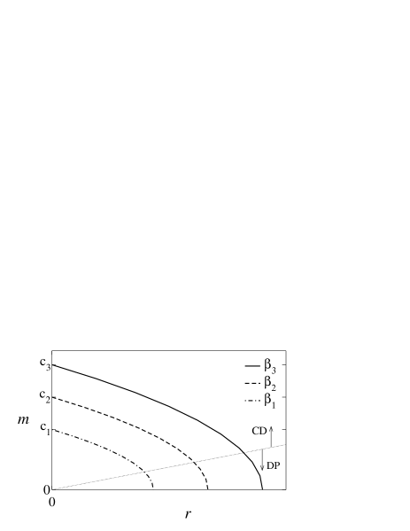
The qualitative behaviour of the model with finite $r$ is shown in Fig. 10. The “dimensionless” parameter that determines the effect of $r$ is the product of the death rate and the relaxation time of the FA model:

$$r\tau\simeq re^{3\beta}\equiv R,$$ (37)

which defines $R$. At any finite $\beta$ there is a directed percolation transition to an active state, which occurs when $R$ is of order unity. This transition is accompanied by a diverging static correlation length:

$$\langle n_{i\tau}n_{j\tau}\rangle-\langle n_{i\tau}\rangle^{2}\sim|r_{i}-r_{j}|^{z\theta-d}e^{|r_{i}-r_{j}|/\xi_{\mathrm{DP}}},$$ (38)

where $\xi_{\mathrm{DP}}$ is the length scale that diverges at the transition and $z$ and $\theta$ are DP exponents Hinrichsen (2000) (the dimensionality is $d=1$). On the other hand, if $R=0$ then there is a transition at $c=0$ that is controlled by the coagulation-diffusion fixed point. In that case we have

$$\langle n_{i\tau}n_{j\tau}\rangle-\langle n_{i\tau}\rangle^{2}\sim\delta_{ij}.$$ (39)

for all $c$. We show in the figure how the crossover into the DP critical region is always relevant if $R$ is finite, but does not affect the behaviour if $R=0$. We note that between two and four dimensions a similar picture holds, but the scaling at $R=0$ will be Gaussian Jack et al. (2006).

Turning to the dynamical action, we define

$$\mathcal{E}^{(r)}_{\mathrm{traj}}=\mathcal{N}_{\mathrm{upflips}}\ln(e^{\beta})+\mathcal{N}_{\mathrm{downflips}}^{(\mathrm{death})}\ln(1/r)$$

$$+\int_{0}^{t_{\rm obs}}\!\!\!\mathrm{d}\tau\,\sum_{i}\left\{f_{\mathrm{i\tau}}[(1-n_{i\tau})e^{-\beta}+n_{i\tau}(1-r)]+n_{i\tau}r\right\}$$

by analogy with (28), where we have set the coarse-graining time scale $\delta t=1$ for ease of writing. Equations (30-33) remain true since facilitated spins are still equilibrated at a density close to $c=(1+e^{\beta})^{-1}$ (but note that the mean density in the system will be less than $c$: the death process reduces the mean density).

In Fig. 9 we plot the distribution of the action density at finite $r$ and compare it with the behaviour of the $b$-ensemble. Since the system does not obey detailed balance the TPS procedure becomes inefficient: data at finite $r$ is obtained by simple binning and histogramming. In the $b$-ensemble, the mean action is reduced as the (finite) system crosses over from an active to an inactive state (this crossover would be a first order phase transition in the thermodynamic limit). On the other hand, increasing $r$ reduces the gradient of the exponential tail and the mean action, as the second order phase transition is approached (at $r_{c}$).

Figure 11: Sample trajectories at $R=0.1$ with conditions otherwise similar to Fig. 3 ($\beta=1$, $L=60$ $t_{\rm obs}=320$). (Left) Sample from centre of distribution. (Right) Sample with $m_{\mathrm{traj}}\sim\langle m\rangle/2$. Clearly there are more large inactive regions in these trajectories than in those of Fig. 1; increasing $R$ from zero leads to proliferation of large “bubbles”.

The key difference between the FA model and its generalisation to finite $r$ is that the surface tension and mean magnetisation decouple at finite $r$. On reducing the temperature in the FA model ($r=0$, $c\to 0$) we have $\sigma_{1}\sim\langle m\rangle\sim c$, so the typical bubble size $\sigma_{1}^{-1}$ scales in the same way as the inverse density of up spins. In contrast, as we approach the DP fixed point ($\beta$ finite, $r\to r_{\mathrm{crit}}$) then we have

$$\sigma_{1}\sim(r-r_{\mathrm{crit}})^{\nu_{\mathrm{DP}}},\qquad\langle m\rangle\sim(r-r_{\mathrm{crit}})^{\beta_{\mathrm{DP}}}$$ (41)

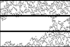
where $(\nu_{\mathrm{DP}},\beta_{\mathrm{DP}})\simeq(1.1,0.3)$ are the exponents of the DP fixed point Hinrichsen (2000) ($\beta_{\mathrm{DP}}$ should not be confused with the parameter $\beta$ that enters the transition probabilities). As criticality is approached, the mean bubble size increases much faster than the inverse density since $\nu_{\mathrm{DP}}>\beta_{\mathrm{DP}}$. The up spins cluster together, leaving large inactive regions consisting only of down spins. Introducing the death process drives the system towards a phase separation into active and inactive regions of space-time. This can be seen in the trajectories of Fig. 11.

Finally, we note that the critical DP scaling leads to a crossover at small $R$, when the typical size of inactive regions exceeds the observation box ($\sigma_{1}L\sim 1$). In that case, $P(\rho_{\mathcal{E}})$ acquires a second peak at zero magnetisation (see the largest value of $R$ in Fig. 9). This is analogous to the situation for small boxes ($cL<1$) in the FA case (recall Fig. 6). In the thermodynamic language, it corresponds to a second minimum in the free energy, as would be observed near a first order phase transition. Here, the phase transition is second order, but the finite size of the observation box means that the divergence of the correlation length is cut off at the size of the observation box.

Thus, we have shown that adding a death process to the FA model strengthens the analogy between trajectory statistics and the statistical mechanics of phase coexistence. In the FA model, the only length scale is the inverse density of up spins; if $r$ is finite then a new length scale appears: the DP correlation length. This second length scale allows the density of active regions to decouple from their separation, leading to richer behaviour than that of the FA model (which corresponds to the particular case of the phase coexistence in which the two length scales are equal).

Throughout this article, we have emphasised the broad applicability of the idea of space-time phase coexistence by focussing on general features of the models, such as microscopic reversibility and reducibility of the dynamics. We expect the behaviour described here to be generic in kinetically constrained models with reducible dynamics Ritort and Sollich (2003); Eisinger and Jackle (1993); Garrahan and Chandler (2003); Berthier and Garrahan (2005); KA- . More generally, the extent to which this behaviour can be observed in real structural glass-formers remains an open question.

Appendix A Transition path sampling

We calculated probability distributions for various observables in the FA model: these were obtained by a combination of transition path sampling (TPS) Bolhuis et al. (2002) and umbrella sampling Frenkel and Smit (2001). Here we give a brief description of the procedure used.

Transition path sampling is a Monte Carlo procedure applied to trajectories of a dynamical system (a trajectory is a particular realisation of the dynamics). We use it to efficiently sample restricted ensembles of trajectories. The procedure is well-established Bolhuis et al. (2002), but we present some information regarding its application to the FA model for completeness.

Suppose that we wish to sample trajectories with magnetisation $m$ smaller than some reference value $m_{1}$. The simplest way to do this is to generate statistically independent trajectories, accepting only those that satisfy the restriction $m<m_{1}$. However, if $m_{1}$ is much smaller than the mean of $m$ then this is inefficient.

Instead, we can generate unbiased trajectories satisfying the restriction by deforming a set of initial trajectories, as long as the deformations satisfy detailed balance with respect to the probability distribution within the constrained ensemble of trajectories. Such deformations are called TPS moves. One possibility is to take a trajectory of length $t_{\rm obs}$ and keep only the part with $t<(xt_{\rm obs})$ with $0<x<1$; we the generate the rest of the trajectory using the dynamical rules prescribed for the system (we use a continuous time Monte Carlo algorithm Newman and Barkema (1999)). If the new trajectory has $m<m_{1}$ then it replaces the old one; otherwise the move is rejected and we retain the old trajectory. This is a “shooting” move Bolhuis et al. (2002). We couple this the move with the reverse procedure in which we discard the part of the trajectory with $t>(xt_{\rm obs})$ and regenerate the rest of the trajectory by propagating backwards in time (since we have detailed balance then the steady state of the FA model is invariant under time-reversal, so this is a valid way to generate unbiased trajectories).

In addition to these moves, we also use “shifting” moves Bolhuis et al. (2002) in which we shift the trajectory in time, discarding the parts of the new trajectory with $t<0$ or $t>t_{\rm obs}$. We then regenerate the remaining parts of the new trajectory. We find that this combination of moves is quite efficient for exploring the restricted ensembles of interest.

Appendix B Umbrella sampling

We use umbrella sampling Frenkel and Smit (2001) to calculate probability distributions by measuring ratios such as

$$P_{i,i+1}=\frac{P(m<m_{i+1})}{P(m<m_{i})}$$ (42)

where $m_{i}$ and $m_{i+1}$ are two cutoffs for the variable $m$ with $m_{i+1}<m_{i}$.

Consider an ensemble of all allowed trajectories for the system, with their statistical weights. In order to measure $P_{i,i+1}$ we sample a restricted ensemble which contains only trajectories with $m<m_{i}$; these trajectories have the same weights as they would have in the original ensemble. We then measure the probability that $m<m_{i+1}$ within the restricted ensemble: this probability is equal to $P_{i,i+1}$.

Our procedure is as follows:

1. Start with a representative set of trajectories from the unrestricted ensemble.

2. Choose an ordered set of cutoff magnetisations $(m_{1}>m_{2}>\dots>m_{p})$ for which we will calculate the probabilities $P_{i,i+1}$.

3. Explore the unrestricted ensemble, measuring the fraction of trajectories with $m<m_{1}$. (This is done by sampling independent trajectories.)

4. Once we have a good enough estimate for $P(m<m_{1})$, start a restricted ensemble with trajectories satisfying $m<m_{1}$. Typically we store $N_{e}=100$ such trajectories.

5. Explore the restricted ensemble using TPS, measuring the fraction of trajectories with $m<m_{2}$. Typically this takes $N_{m}=100-10000$ TPS moves per ensemble member.

6. Once we have a good enough estimate for $P_{12}$, we discard all trajectories with $m>m_{2}$ and replace them by trajectories with $m<m_{2}$. These trajectories are generated by continuing the TPS procedure and accepting all trajectories that satisfy the new constraint. The resulting set of trajectories are not statistically independent so we equilibrate the new ensemble by allowing it to evolve from the biased initial condition. Typically we use around $N_{m}$ TPS moves per ensemble member. We test for equilibration by tracking the fraction of trajectories with $m<m_{3}$, since this will be the quantity that we will measure on the next step.

7. We then repeat steps 5 and 6 for increasingly restricted ensembles. At each step, we measure $P_{i,i+1}$.

Once we have the $P(m<m_{1})$ and the set of $P_{i,i+1}$ then it is simple to reconstruct the probability distribution of the observable $m$.

References

- Rev (a) For reviews see: M.D. Ediger, C.A. Angell and S.R. Nagel, J. Phys. Chem. 100 13200 (1996); C.A. Angell, Science 267, 1924 (1995); P.G. Debenedetti and F.H. Stillinger, Nature 410, 259 (2001).
- Rev (b) For reviews see: H. Sillescu, J. Non-Cryst. Solids 243, 81 (1999); M.D. Ediger, Annu. Rev. Phys. Chem. 51, 99 (2000); S.C. Glotzer, J. Non-Cryst. Solids, 274, 342 (2000); R. Richert, J. Phys. Condens. Matter 14, R703 (2002); H. C. Andersen, Proc. Natl. Acad. Sci. U. S. A. 102, 6686 (2005).
- Merolle et al. (2005) M. Merolle, J. P. Garrahan, and D. Chandler, Proc. Natl. Acad. Sci. U. S. A. 102, 10837 (2005).
- Huang and Chandler (2000) D. M. Huang and D. Chandler, Phys. Rev. E 61, 1501 (2000).
- Clusel et al. (2004) M. Clusel, J. Y. Fortin, and P. C. W. Holdsworth, Phys. Rev. E 70, 046112 (2004).
- Garrahan and Chandler (2002) J. P. Garrahan and D. Chandler, Phys. Rev. Lett. 89, 035704 (2002).
- Ritort and Sollich (2003) F. Ritort and P. Sollich, Adv. Phys. 52, 219 (2003).
- (8) D. Ruelle, Thermodynamic Formalism (Addison-Wesley, Reading, 1978).
- (9) V. Lecomte, C. Appert-Roland and F. van Wijland, cond-mat/0606211
- Fredrickson and Andersen (1984) G. H. Fredrickson and H. C. Andersen, Phys. Rev. Lett. 53, 1244 (1984).
- Jack et al. (2006) R. L. Jack, P. Mayer, and P. Sollich, J. Stat. Mech. (2006), P03006.
- Hinrichsen (2000) H. Hinrichsen, Adv. Phys. 49, 815 (2000).
- Harrowell (1993) P. Harrowell, Phys. Rev. E 48, 4359 (1993).
- Garrahan and Chandler (2003) J. P. Garrahan and D. Chandler, Proc. Natl. Acad. Sci. U. S. A. 100, 9710 (2003).
- Jung et al. (2004) Y.-J. Jung, J. P. Garrahan, and D. Chandler, Phys. Rev. E 69, 061205 (2004).
- Toninelli et al. (2005) C. Toninelli, M. Wyart, L. Berthier, G. Biroli, and J. P. Bouchaud, Phys. Rev. E 71, 041505 (2005).
- Bertin et al. (2005) E. Bertin, J. P. Bouchaud, and F. Lequeux, Phys. Rev. Lett. 95, 015702 (2005).
- (18) C. Chamon, P. Charbonneau, L. F. Cugliandolo, D. R. Reichman and M. Selitto, J. Chem. Phys. 121, 10120 (2004)
- (19) A. Duri, H. Bissig, V. Trappe, L. Cipelletti. Phys. Rev. E 72, 051401 (2005).
- (20) L. Maibaum, Ph.D. thesis (University of California at Berkeley, 2005).
- Bolhuis et al. (2002) P. G. Bolhuis, D. Chandler, C. Dellago, and P. L. Geissler, Ann. Rev. Phys. Chem. 53, 291 (2002).
- Frenkel and Smit (2001) D. Frenkel and B. Smit, Understanding molecular simulation (Academic Press, 2001).
- Jung et al. (2005) Y.-J. Jung, J. P. Garrahan, and D. Chandler, J. Chem. Phys. 123, 084509 (2005).
- (24) G. Parisi, Statistical Field Theory, (Addison-Wesley, New York, 1988).
- (25) C. Giardina, J. Kurchan and L. Peliti, Phys. Rev. Lett 96, 120603 (2006).
- Eisinger and Jackle (1993) S. Eisinger and J. Jackle, J. Stat. Phys. 73, 643 (1993).
- Berthier and Garrahan (2005) L. Berthier and J. P. Garrahan, J. Phys. Chem. B 109, 6916 (2005).
- (28) W. Kob and H.C. Andersen, Phys. Rev. E 48, 4364 (1993); J. Jäckle and A. Krönig, J. Phys. Condens. Matter 6, 7633 (1994); A.C. Pan, J.P. Garrahan and D. Chandler, Phys. Rev. E 72, 041106 (2005); C. Toninelli, G. Biroli and D.S. Fisher, J. Stat. Phys. 120, 167 (2005); C. Toninelli, G. Biroli and D.S. Fisher, Phys. Rev. Lett. 96, 035702 (2006).
- Newman and Barkema (1999) M. E. J. Newman and G. T. Barkema, Monte Carlo Methods in Statistical Physics (Oxford University Press, 1999).