Exact solutions for models of evolving networks with addition and deletion of nodes

Abstract

There has been considerable recent interest in the properties of networks, such as citation networks and the worldwide web, that grow by the addition of vertices, and a number of simple solvable models of network growth have been studied. In the real world, however, many networks, including the web, not only add vertices but also lose them. Here we formulate models of the time evolution of such networks and give exact solutions for a number of cases of particular interest. For the case of net growth and so-called preferential attachment—in which newly appearing vertices attach to previously existing ones in proportion to vertex degree—we show that the resulting networks have power-law degree distributions, but with an exponent that diverges as the growth rate vanishes. We conjecture that the low exponent values observed in real-world networks are thus the result of vigorous growth in which the rate of addition of vertices far exceeds the rate of removal. Were growth to slow in the future, for instance in a more mature future version of the web, we would expect to see exponents increase, potentially without bound.

I Introduction

The study of networks has attracted a substantial amount of attention from the physics community in the last few years AB02 ; DM02 ; Newman03d , in part because of networks’ broad utility as representations of real-world complex systems and in part because of the demonstrable successes of physics techniques in shedding light on networked phenomena. One topic that has been the subject of a particularly large volume of work is growing networks, such as citation networks Price65 ; Redner98 and the worldwide web AJB99 ; Kleinberg99b . Perhaps the best-known body of work on this topic is that dealing with “preferential attachment” models Price76 ; BA99b , in which vertices are added to a network with edges that attach to preexisting vertices with probabilities depending on those vertices’ degrees. When the attachment probability is precisely linear in the degree of the target vertex the resulting degree sequence for the network follows a Yule distribution in the limit of large network size, meaning it has a power-law tail Price76 ; BA99b ; KRL00 ; DMS00 ; BRST01 . This case is of special interest because both citation networks and the worldwide web are observed to have degree distributions that approximately follow power laws.

The preferential attachment model may be quite a good model for citation networks, which is one of the cases for which it was originally proposed Price76 ; KRL00 . For other networks, however, and especially for the worldwide web, it is, as many authors have pointed out, necessarily incomplete DM00b ; AB00a ; KR02a ; Tadic02 ; GSM05 . On the web there are clearly other processes taking place in addition to the deposition of vertices and edges. In particular, it is a matter of common experience that vertices (i.e., web pages) are often removed from the web, and with them the links that they had to other pages. Models of this process have been touched upon occasionally in the literature CL04 ; CFV04 and the evidence suggests that in some cases vertex deletion affects the crucial power-law behavior of the degree distribution, while in other cases it does not.

In this paper, we study the general process in which a network grows (or, potentially, shrinks) by the constant addition and removal of vertices and edges. We show that a class of such processes can be solved exactly for the degree distributions they generate by solving differential equations governing the probability generating functions for those distributions. In particular, we give solutions for three example problems of this type, having uniform or preferential attachment, and having stationary size or net growth. The case of uniform attachment and stationary size is of interest as a possible model for the structure of peer-to-peer filesharing networks, while the preferential-attachment stationary-size case displays a nontrivial stretched exponential form in the tail of the degree distribution. Our solution of the preferential attachment case with net growth confirms earlier results indicating that this process generates a power-law distribution, although the exponent of the power-law diverges as the growth rate tends to zero, giving degree distributions that are numerically indistinguishable from exponential for small growth rates. This suggests that the clear power law seen in the real worldwide web is a signature of a network whose rate of vertex accrual far outstrips the rate at which vertices are removed. The relative rates of addition and removal could, however, change as the web matures, possibly leading to a loss of power-law behavior at some point in the future.

II The model

Consider a network that evolves by the addition and removal of vertices. In each unit of time, we add a single vertex to the network and remove $r$ vertices. When a vertex is removed so too are all the edges incident on that vertex, which means that the degrees of the vertices at the other ends of those edges will decrease. Non-integer values of $r$ are permitted and are interpreted in the usual stochastic fashion. (For example, values $r<1$ can be interpreted as the probability per unit time that a vertex is removed.) The value $r=1$ corresponds to a network of fixed size in which there is vertex turnover but no growth; values $r<1$ correspond to growing networks. In principle one could also look at values $r>1$, which correspond to shrinking networks, and the methods derived here are applicable to that case. However, we are not aware of any real-world examples of shrinking networks in which the asymptotic degree distribution is of interest, so we will not pursue the shrinking case here.

We make two further assumptions, which have also been made by most previous authors in studying these types of systems: (1) that all vertices added have the same initial degree, which we denote $c$; (2) that the vertices removed are selected uniformly at random from the set of all extant vertices. Note however that we will not assume that the network is uncorrelated (i.e., that it is a random multigraph conditioned on its degree distribution as in the so-called configuration model). In general the networks we consider will have correlations among the degrees of their vertices but our solutions will nonetheless be exact.

Let $p_{k}$ be the fraction of vertices in the network at a given time that have degree $k$. By definition, $p_{k}$ has the normalization

$$\sum_{k=0}^{\infty}p_{k}=1.$$ (1)

Our primary goal in this paper will to evaluate exactly the degree distribution $p_{k}$ for various cases of interest.

Although the form of $p_{k}$ is, as we will see, highly nontrivial in most cases, the mean degree of a vertex $\langle k\rangle=\sum_{k=0}^{\infty}kp_{k}$ is easily derived in terms of the parameters $r$ and $c$. The mean number of vertices added to the network per unit time is $1-r$. The mean number of edges removed when a randomly chosen vertex is removed from the network is by definition $\langle k\rangle$. Thus the mean number of edges added to the network per unit time is $c-r\langle k\rangle$. For a graph of $m$ edges and $n$ vertices, the mean degree is $\langle k\rangle=2m/n$. After time $t$ we have $n=(1-r)t$ and, assuming that $\langle k\rangle$ has an asymptotically constant value, $m=(c-r\langle k\rangle)t$. Thus

$$\langle k\rangle=2{c-r\langle k\rangle\over 1-r},$$ (2)

or, rearranging,

$$\langle k\rangle={2c\over 1+r}.$$ (3)

In the special case $r=1$ of a constant-size network, this gives $\langle k\rangle=c$, which is clearly the correct answer.

We must also consider how an added vertex chooses the $c$ other vertices to which it attaches. Let us define the attachment kernel $\pi_{k}$ to be $n$ times the probability that a given edge of a newly added vertex attaches to a given preexisting vertex of degree $k$. The factor of $n$ here is convenient, since it means that the total probability that the given edge attaches to any vertex of degree $k$ is simply $\pi_{k}p_{k}$. Since each edge must attach to a vertex of some degree, this also immediately implies that the correct normalization for $\pi_{k}$ is

$$\sum_{k=0}^{\infty}\pi_{k}p_{k}=1.$$ (4)

For the particular case of $\pi_{k}\propto k$ and $r<1$, which we consider in Section III.3, models similar to ours have been studied previously by Chung and Lu CL04 and by Cooper, Frieze, and Vera CFV04 . The results reported by these authors are mostly of a different nature to ours, but there are some overlaps, which we discuss at the appropriate point.

II.1 Rate equation

Given these definitions, the evolution of the degree distribution is governed by a rate equation as follows. If there are at total of $n$ vertices in the network at a given time then the number of vertices with degree $k$ is $np_{k}$. One unit of time later this number is $(n+1-r)p_{k}^{\prime}$, where $p_{k}^{\prime}$ is the new value of $p_{k}$. Then

$$(n+1-r)p_{k}^{\prime} = np_{k}+\delta_{kc}+c\pi_{k-1}p_{k-1}-c\pi_{k}p_{k}$$ (5)

$${}+r(k+1)p_{k+1}-rkp_{k}-rp_{k}.$$

The term $\delta_{kc}$ in Eq. (5) represents the addition of a vertex of degree $c$ to the network. The terms $c\pi_{k-1}p_{k-1}$ and $-c\pi_{k}p_{k}$ describe the flow of vertices from degree $k-1$ to $k$ and from $k$ to $k+1$ as they gain extra edges when newly added vertices attach to them. The terms $(k+1)p_{k+1}$ and $-kp_{k}$ describe the flow from degree $k+1$ to $k$ and from $k$ to $k-1$ as vertices loose edges when one of their neighbors is removed from the network. And the term $-rp_{k}$ represents the removal with probability $r$ of a vertex with degree $k$. Contributions from processes in which a vertex gains or loses two or more edges in a single unit of time vanish in the limit of large $n$ and have been neglected.

We will be interested in the asymptotic form of $p_{k}$ in the limit of large times for a given $\pi_{k}$. Setting $p_{k}^{\prime}=p_{k}$ in (5) gives

$$\delta_{kc} + c\pi_{k-1}p_{k-1}-c\pi_{k}p_{k}$$ (6)

$$+ r(k+1)p_{k+1}-rkp_{k}-p_{k}=0,$$

whose solution we can write in terms of generating functions as follows. Let us define

$$f(z) = \sum_{k=0}^{\infty}\pi_{k}p_{k}z^{k},$$ (7)

$$g(z) = \sum_{k=0}^{\infty}p_{k}z^{k}.$$ (8)

Then, upon multiplying both sides of (6) by $z^{k}$ and summing over $k$ (with the convention that $p_{-1}=0$), we derive a differential equation for $g(z)$ thus:

$$r(1-z){\mathrm{d}g\over\mathrm{d}z}-g(z)-c(1-z)f(z)+z^{c}=0.$$ (9)

Note also that we can easily generalize our model to the case where the degrees of the vertices added are not all identical but are instead drawn at random from some distribution $r_{k}$. In that case, we simply replace $\delta_{kc}$ in Eq. (6) with $r_{k}$ and $z^{c}$ in Eq. (9) with the generating function $h(z)=\sum_{k}r_{k}z^{k}$.

In the following sections we solve Eq. (9) for a number of different choices of the attachment kernel $\pi_{k}$. Note that, since the definitions of both $f(z)$ and $g(z)$ incorporate the unknown distribution $p_{k}$, we must in general solve implicitly for $g(z)$ in terms of $f(z)$. In all of the cases of interest to us here, however, it turns out to be straightforward to derive a explicit equation for $g(z)$ as a special case of (9).

III Solutions for specific cases

In this section we study three specific examples of the class of models defined in the preceding section, namely linear preferential attachment models ($\pi_{k}\propto k$) for both growing and fixed-size networks, and uniform attachment ($\pi_{k}=\mbox{constant}$) for fixed size. As we will see, each of these cases turns out to have interesting features.

III.1 Uniform attachment and constant size

For the first of our example models we study the case where the size of the network is constant ($r=1$) and in which each vertex added chooses the $c$ others to which it attaches uniformly at random. This means that $\pi_{k}$ is constant, independent of $k$, and, combining Eqs. (1) and (4), we immediately see that the correct normalization for the attachment kernel is $\pi_{k}=1$ for all $k$. Then we have $\pi_{k}p_{k}=p_{k}$ so that $f(z)=g(z)$ in (9), which gives

$$\biggl{(}c+{1\over 1-z}\biggr{)}g(z)-{\mathrm{d}g\over\mathrm{d}z}={z^{c}\over 1-z}.$$ (10)

Noting that $(1-z)\mathrm{e}^{-cz}$ is an integrating factor and that $g(z)$ must obey the boundary condition $g(1)=1$, we readily determine that

$$g(z) = {\mathrm{e}^{cz}\over 1-z}\int_{z}^{1}t^{c}\mathrm{e}^{-ct}\>\mathrm{d}t$$ (11)

$$= \frac{\mathrm{e}^{cz}}{1-z}c^{-(c+1)}\bigl{[}\Gamma(c+1,cz)-\Gamma(c+1,c)\bigr{]},\quad$$

where

$$\Gamma(c+1,x)=\int_{x}^{\infty}t^{c}\mathrm{e}^{-t}\>\mathrm{d}t.$$ (12)

is the incomplete $\Gamma$-function.

One can easily check that this gives a mean degree $g^{\prime}(1)=c$, as it must, and that the variance of the degree $g^{\prime\prime}(1)+g^{\prime}(1)-c^{2}$ is equal to $\frac{2}{3}c$, indicating a tightly peaked degree distribution.

To obtain an explicit expression for the degree distribution, we make use of

$$\Gamma(c+1,x) = \Gamma(c+1)\,\mathrm{e}^{-x}\sum_{m=0}^{c}\frac{x^{m}}{m!},$$ (13)

$$\mathrm{e}^{x} = \sum_{m=0}^{\infty}\frac{x^{m}}{m!},$$ (14)

$$(1-z)^{-1} = \sum_{k=0}^{\infty}z^{k},$$ (15)

to write

$$g(z) = c^{-(c+1)}$$

$${}\times\sum_{k=0}^{\infty}z^{k}\biggl{[}\Gamma(c+1)\sum_{m=0}^{c}{(cz)^{m}\over m!}-\Gamma(c+1,c)\sum_{m=0}^{\infty}{(cz)^{m}\over m!}\biggr{]}.$$

The $z$-dependence in the first term of this expression can be rewritten

$$\sum_{k=0}^{\infty}z^{k}\sum_{m=0}^{c}{(cz)^{m}\over m!} = \sum_{m=0}^{c}\sum_{k=m}^{\infty}z^{k}{c^{m}\over m!}$$ (17)

$$= \sum_{k=0}^{\infty}z^{k}\sum_{m=0}^{\min(k,c)}{c^{m}\over m!}$$

$$= \mathrm{e}^{c}\sum_{k=0}^{\infty}z^{k}{\Gamma\bigl{(}\min(k,c)+1,c\bigr{)}\over\Gamma\bigl{(}\min(k,c)+1\bigr{)}},\quad{}$$

where $\min(k,c)$ denotes the smaller of $k$ and $c$ and we have again employed (13). A similar sequence of manipulations leads to an expression for the second term also, thus:

$$\sum_{k=0}^{\infty}z^{k}\sum_{m=0}^{\infty}{(cz)^{m}\over m!}=\mathrm{e}^{c}\sum_{k=0}^{\infty}z^{k}{\Gamma(k+1,c)\over\Gamma(k+1)}.$$ (18)

Combining these identities with (LABEL:eq:gzrewrite), it is then a simple matter to read off the term in $g(z)$ involving $z^{k}$, which is by definition our $p_{k}$. We find two separate expressions for the cases of $k$ above or below $c$:

$$p_{k} = {\mathrm{e}^{c}\over c^{c+1}}\bigl{[}\Gamma(c+1)-\Gamma(c+1,c)\bigr{]}{\Gamma(k+1,c)\over\Gamma(k+1)},$$ (19)

$$\hskip 130.0002pt\mbox{for $k<c$},$$

and

$$p_{k}={\mathrm{e}^{c}\over c^{c+1}}\Gamma(c+1,c)\biggl{[}1-{\Gamma(k+1,c)\over\Gamma(k+1)}\biggr{]},\quad\mbox{for $k\geq c$}.$$ (20)

Note that the quantity $\Gamma(k+1,c)/\Gamma(k+1)$ appearing in both these expressions is the probability that a Poisson-distributed variable with mean $c$ is less than or equal to $k$. Thus the degree distribution has a tail that decays as the cumulative distribution of such a Poisson variable, implying that it falls off rapidly. To see this more explicitly, we note that for fixed $c$ and $k\gg c$

$$p_{k}={\Gamma(c+1,c)\over c^{c+1}}\!\!\sum_{m=k+1}^{\infty}{c^{m}\over m!}\simeq{\Gamma(c+1,c)\over\Gamma(k+2)}c^{k-c},$$ (21)

since the sum is strongly dominated in this limit by its first term. Applying Stirling’s approximation, $\Gamma(x)\simeq(x/\mathrm{e})^{x}\sqrt{2\pi/x}$, this gives

$$p_{k}\simeq{\Gamma(c+1,c)\over c^{c}}k^{-3/2}\mathrm{e}^{k}\biggl{(}{c\over k}\biggr{)}^{k},$$ (22)

which decays substantially faster asymptotically than any exponential.

Figure 1: The degree distribution of our model for the case of uniform attachment ($\pi_{k}=\mbox{constant}$) with fixed size $n=50\,000$ and $c=10$. The points represent data from numerical simulations and the solid line is the analytic solution.

As a check on these calculations, we have performed extensive computer simulations of the model. In Fig. 1 we show results for the case $c=10$, along with the exact solution from Eqs. (19) and (20). As the figure shows, the agreement between the two is excellent.

Before moving on to other issues, we note a different and particularly simple case of a growing network with uniform attachment, the case in which the vertices added have a Poisson degree distribution $c^{k}\mathrm{e}^{-c}/k!$ with mean $c$. In that case the factor of $z^{c}$ in Eq. (10) is replaced with the generating function $h(z)$ for the Poisson distribution:

$$h(z)=\sum_{k=0}^{\infty}{c^{k}\mathrm{e}^{-c}\over k!}z^{k}=\mathrm{e}^{c(z-1)},$$ (23)

and the solution, Eq. (11), becomes

$$g(z)={\mathrm{e}^{cz}\over 1-z}\int_{z}^{1}h(t)\,\mathrm{e}^{-ct}\>\mathrm{d}t=\mathrm{e}^{c(z-1)},$$ (24)

which is itself the generating function for a Poisson distribution. Thus we see particularly clearly in this case that the equilibrium degree distribution in the steady-state uniform attachment network is sharply peaked with a Poisson tail. In fact, the network in this case is simply an uncorrelated random graph of the type famously studied by Erdős and Rényi ER60 . It is straightforward to see that if one starts with such a graph and randomly adds and removes vertices with Poisson distributed degrees, the graph remains an uncorrelated random graph with the same degree distribution, and hence this distribution is necessarily the fixed point of the evolution process, as the solution above demonstrates.

III.2 Preferential attachment and constant size

Our next example adds an extra degree of complexity to the picture: we consider vertices that attach to others in proportion to their degree, the so-called “preferential attachment” mechanism BA99b . This implies that our attachment kernel $\pi_{k}$ is linear in the degree, $\pi_{k}=Ak$ for some constant $A$. The normalization requirement (4) then implies that

$$\sum_{k=0}^{\infty}\pi_{k}p_{k}=A\sum_{k=0}^{\infty}kp_{k}=A\langle k\rangle=1,$$ (25)

and hence $A=1/\langle k\rangle$. For the moment, let us continue to focus on the case $r=1$ of constant network size, in which case $\langle k\rangle=c$ (Eq. (3)) and

$$\pi_{k}={k\over c}.$$ (26)

Then

$$f(z)={1\over c}\sum_{k=0}^{\infty}kp_{k}z^{k}={z\over c}\,g^{\prime}(z),$$ (27)

and Eq. (9) becomes

$${g(z)\over(1-z)^{2}}-{\mathrm{d}g\over\mathrm{d}z}={z^{c}\over(1-z)^{2}}.$$ (28)

The appropriate integrating factor in this case is $\mathrm{e}^{-1/(1-z)}$, which, in conjunction with the boundary condition $g(1)=1$, gives

$$g(z)=e^{1/(1-z)}\int_{z}^{1}\frac{t^{c}}{(1-t)^{2}}\mathrm{e}^{-1/(1-t)}\>\mathrm{d}t.$$ (29)

Changing the variable of integration to $y=1/(1-t)$ this expression can be written

$$g(z) = \mathrm{e}^{1/(1-z)}\int_{1/(1-z)}^{\infty}\left(1-\frac{1}{y}\right)^{\!c}\mathrm{e}^{-y}\,\mathrm{d}y$$ (30)

$$= \mathrm{e}^{1/(1-z)}\sum_{s=0}^{c}(-1)^{s}{c\choose s}\int_{1/(1-z)}^{\infty}\frac{\mathrm{e}^{-y}}{y^{s}}\,\mathrm{d}y$$

$$= 1+\mathrm{e}^{1/(1-z)}\sum_{s=1}^{c}(-1)^{s}{c\choose s}\,\Gamma\!\left(1-s,\frac{1}{1-z}\right).\qquad{}$$

where $\Gamma(1-s,x)=\int_{x}^{\infty}e^{-y}\,y^{-s}\,\mathrm{d}y$ is again the incomplete $\Gamma$-function, here appearing with a negative first argument.

A useful identify for the case $s\geq 1$ can be derived by integrating by parts thus:

$$\Gamma(-s,x)=\frac{1}{s}\biggl{[}\frac{\mathrm{e}^{-x}}{x^{s}}-\Gamma(1-s,x)\biggr{]}.$$ (31)

Iterating this expression then gives

$$\Gamma(1-s,x)=-\frac{(-1)^{s}}{(s-1)!}\biggl{[}\Gamma(0,x)+\mathrm{e}^{-x}\!\sum_{m=1}^{s-1}\frac{(-1)^{m}(m-1)!}{x^{m}}\biggr{]}.$$ (32)

($\Gamma(0,x)=\int_{x}^{\infty}(\mathrm{e}^{-y}/y)\,\mathrm{d}y$ is also known as the exponential integral function $-\mathop{\mathrm{Ei}}(-x)$.) Applying this identity to (30) gives

$$g(z) = 1-\sum_{s=1}^{c}{c\choose s}\frac{1}{(s-1)!}$$ (33)

$${}\times\biggl{[}\mathrm{e}^{1/(1-z)}\,\Gamma\!\biggl{(}0,\frac{1}{1-z}\biggr{)}+\sum_{m=1}^{s-1}(-1)^{m}(m-1)!\,(1-z)^{m}\biggr{]}$$

$$= q(z)-A_{c}\,\mathrm{e}^{1/(1-z)}\,\Gamma\!\biggl{(}0,\frac{1}{1-z}\biggr{)},$$

where $q(z)$ is a polynomial of degree $c-1$ and $A_{c}=\sum_{s=1}^{c}{c\choose s}/(s-1)!$ depends only on $c$. For $k\geq c$, then, the degree distribution $p_{k}$ is given by the coefficients of $z^{k}$ in $-A_{c}\,\mathrm{e}^{1/(1-z)}\,\Gamma\bigl{(}0,1/(1-z)\bigr{)}$. We determine these coefficients as follows. Changing the variable of integration to $x=y-z/(1-z)$, we find

$$-\mathrm{e}^{1/(1-z)}\,\Gamma\!\left(0,\frac{1}{1-z}\right)=-\mathrm{e}\int_{1}^{\infty}\frac{\mathrm{e}^{-x}}{x+z/(1-z)}\,\mathrm{d}x.$$ (34)

Then we expand the integrand to get

$$\frac{1}{x+z/(1-z)}=\frac{1}{x}-\sum_{k=1}^{\infty}\left(1-\frac{1}{x}\right)^{\!k-1}\frac{z^{k}}{x^{2}}.$$ (35)

Commuting the sum and the integral, we obtain

$$-\mathrm{e}^{1/(1-z)}\,\Gamma\!\left(0,\frac{1}{1-z}\right)=\sum_{k=0}^{\infty}a_{k}z^{k},$$ (36)

where

$$a_{0}=-\mathrm{e}\int_{1}^{\infty}\frac{\mathrm{e}^{-x}}{x}\,\mathrm{d}x=-\mathrm{e}\,\Gamma(0,1),$$ (37)

and for $k\geq 1$

$$a_{k}=\mathrm{e}\int_{1}^{\infty}\left(1-\frac{1}{x}\right)^{\!k-1}\frac{\mathrm{e}^{-x}}{x^{2}}\,\mathrm{d}x.$$ (38)

Integrating by parts, we obtain a slightly simpler expression,

$$a_{k}=\frac{\mathrm{e}}{k}\int_{1}^{\infty}\left(1-\frac{1}{x}\right)^{\!k}\mathrm{e}^{-x}\,\mathrm{d}x.$$ (39)

While the coefficients $a_{k}$ can be expressed exactly using hypergeometric functions, a perhaps more informative approach is to employ a saddle-point expansion. The integrand of (39) is unimodal in the interval between 1 and $\infty$, and peaks at $x=\frac{1}{2}(1+\sqrt{4k+1})\simeq\sqrt{k}$. Approximating the integrand as a Gaussian around this point, we obtain as $k\to\infty$

$$a_{k}\simeq\sqrt{\pi\mathrm{e}}\,k^{-3/4}\,\mathrm{e}^{-2\sqrt{k}}$$ (40)

and $p_{k}=A_{c}\,a_{k}$ for $k\geq c$ as stated above.

Figure 2: The degree distribution for our model in the case of fixed size $n=50\,000$ and $c=10$ with linear preferential attachment. The points represent data from our numerical simulations and the solid line is the analytic solution for $k\geq c$. Note that the tail of the distribution does not follow a power law as in growing networks with preferential attachment, but instead decays faster than a power law, as a stretched exponential.

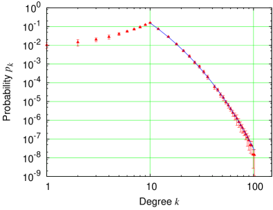
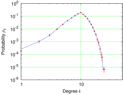
Figure 2 shows the form of this solution for the case $c=10$. Also shown in the figure are results from computer simulations of the model on systems of size $n=50\,000$ with $c=10$, which agree well with the analytic results. The appearance of the stretched exponential in Eq. (40) is worthy of note. We are aware of only a few cases of graphs with stretched exponential degree distributions that have been discussed previously, for instance in growing networks with sublinear preferential attachment KR01 as well as in empirical network data NFB02 .

III.3 Preferential attachment in a growing network

We now come to the third and most complex of our example networks, in which we combine preferential attachment with net growth of the network, $r<1$. (Logically, we should perhaps first solve the case of a growing network without preferential attachment, which in fact we have done. But the solution turns out to have no qualitatively new features to distinguish it from the constant size case and is mathematically tedious besides. Given the large amount of effort it requires and its modest rewards, therefore, we prefer to skip this case and move on to more fertile ground.)

As before, perfect linear preferential attachment implies $\pi_{k}=k/\langle k\rangle$ or

$$\pi_{k}=\mbox{$\frac{1}{2}$}(1+r){k\over c},$$ (41)

where we have made use of Eq. (3). Then $f(z)=(1+r)zg^{\prime}(z)/2c$ and Eq. (9) becomes

$$g(z)-(1-z)\bigl{[}r-\mbox{$\frac{1}{2}$}(1+r)z\bigr{]}\,{\mathrm{d}g\over\mathrm{d}z}=z^{c}.$$ (42)

An integrating factor for the left-hand side in this case is $\bigl{|}(\alpha-z)/(1-z)\bigr{|}^{-2/(1-r)}$ where $\alpha=2r/(1+r)$. (Note that $\alpha<1$ when $r<1$.) Unfortunately, this integrating factor is non-analytic at $z=\alpha$, which makes integrals traversing this point cumbersome. To circumvent this difficulty, we observe that the second term in Eq. (42) vanishes at $z=\alpha$, giving $g(\alpha)=\alpha^{c}$. This provides us with an alternative boundary condition on $g(z)$, allowing us to fix the integrating constant while only integrating up to $z=\alpha$. It is then straightforward to show that

$$g(z) = {2\over 1+r}\biggl{(}{\alpha-z\over 1-z}\biggr{)}^{-2/(1-r)}$$ (43)

$$\quad{}\times\int_{z}^{\alpha}\biggl{(}{\alpha-t\over 1-t}\biggr{)}^{2/(1-r)}\!{t^{c}\>\mathrm{d}t\over(1-t)(\alpha-t)},\quad$$

for $z\leq\alpha$. Since the degree distribution is entirely determined by the behavior of $g(z)$ at the origin, it is adequate to restrict our solution to this regime.

Changing variables to $u=(\alpha-t)/(1-\alpha)$, we find

$$g(z) = {2\over 1+r}\biggl{(}{\alpha-z\over 1-z}\biggr{)}^{1-\gamma}(1-\alpha)^{-1}$$ (44)

$$\times\int_{0}^{{\alpha-z\over 1-\alpha}}\biggl{(}{u\over 1+u}\biggr{)}^{\gamma}\bigl{[}\alpha-(1-\alpha)u\bigr{]}^{c}\>{\mathrm{d}u\over u^{2}},$$

where $\gamma=(3-r)/(1-r)$. If we expand the last factor in the integrand, this becomes

$$g(z) = {2\over 1+r}\sum_{s=0}^{c}(-1)^{s}{c\choose s}(1-\alpha)^{s-1}\alpha^{c-s}$$ (45)

$$\quad{}\times\biggl{(}{\alpha-z\over 1-z}\biggr{)}^{1-\gamma}\int_{0}^{{\alpha-z\over 1-\alpha}}{u^{s+\gamma-2}\over(1+u)^{\gamma}}\>\mathrm{d}u.\qquad$$

We observe the following useful identity:

$$\int_{0}^{x}{u^{\beta}\over(1+u)^{\gamma}}\>\mathrm{d}u=\int_{0}^{x}\biggl{(}{u\over 1+u}\biggr{)}^{\beta}(1+u)^{\beta-\gamma}\>\mathrm{d}u={x^{\beta}\over(\beta-\gamma+1)(1+x)^{\gamma-1}}-{\beta\over\beta-\gamma+1}\int_{0}^{x}{u^{\beta-1}\over(1+u)^{\gamma}}\>\mathrm{d}u,$$ (46)

where the second equality is derived via integration by parts. Setting $\beta=s+\gamma-2$ and $x=(\alpha-z)/(1-\alpha)$ and noting that the last integral has the same form as the first, we can employ this identity iteratively $s-1$ times to get

$$\biggl{(}{\alpha-z\over 1-z}\biggr{)}^{1-\gamma}\int_{0}^{{\alpha-z\over 1-\alpha}}{u^{s+\gamma-2}\over(1+u)^{\gamma}}\>\mathrm{d}u = (-1)^{s+1}{\Gamma(s+\gamma-1)\over\Gamma(s)}$$ (47)

$$\quad{}\times\biggl{[}{1\over\Gamma(\gamma)}\biggl{(}{\alpha-z\over 1-z}\biggr{)}^{1-\gamma}\!\int_{0}^{{\alpha-z\over 1-\alpha}}{u^{\gamma-1}\over(1+u)^{\gamma}}\>\mathrm{d}u+\sum_{m=1}^{s-1}{(-1)^{m}\over\Gamma(\gamma+m)}\biggl{(}{\alpha-z\over 1-z}\biggr{)}^{m}\biggr{]}.\qquad$$

The final sum can be evaluated in closed form in terms of the incomplete $\Gamma$-function, but our primary focus here is on the preceding term. Substituting into Eq. (45), we see that $g(z)=q(z)+A_{c,r}h(z)$, where

$$h(z)=-\biggl{(}\frac{\alpha-z}{1-z}\biggr{)}^{1-\gamma}\int_{0}^{{\alpha-z\over 1-\alpha}}{u^{\gamma-1}\over(1+u)^{\gamma}}\>\mathrm{d}u,$$ (48)

$$A_{c,r}={2\over 1+r}\sum_{s=0}^{c}{c\choose s}(1-\alpha)^{s-1}\alpha^{c-s}\frac{\Gamma(\gamma+s-1)}{\Gamma(\gamma)\Gamma(s)},$$ (49)

and $q(z)$ is a polynomial of order $c-1$ in $z$.

Since $A_{c,r}$ depends only on $c$ and $r$ and $q(z)$ has no terms in $z$ of order $z^{c}$ or higher, the degree distribution for $k\geq c$ is, to within a multiplicative constant, given by the coefficients in the expansion of $h(z)$ about zero. Making the change of variables

$$u={y\over(1-z)/(\alpha-z)-y},$$ (50)

we find that

$$h(z)=-\int_{0}^{1}{y^{\gamma-1}\>\mathrm{d}y\over(1-z)/(\alpha-z)-y},$$ (51)

and expanding the integrand in powers of $z$ we obtain $h(z)=\sum_{k=0}^{\infty}a_{k}z^{k}$ with

$$a_{k} = (1-\alpha)\int_{0}^{1}{(1-y)^{k-1}\over(1-\alpha y)^{k+1}}\,y^{\gamma-1}\>\mathrm{d}y$$ (52)

$$= {\gamma-1\over k}\int_{0}^{1}\biggl{(}{1-y\over 1-\alpha y}\biggr{)}^{k}y^{\gamma-2}\>\mathrm{d}y,$$

for $k\geq 1$, where the second equality follows via an integration by parts.

As in the case of constant size, we can express these coefficients in closed form using special functions, but if we are primarily interested in the form of the tail of the degree distribution then a more revealing approach is to make a further substitution $y=x/k$, giving

$$a_{k}=(\gamma-1)\,k^{-\gamma}\int_{0}^{k}{(1-x/k)^{k}\over(1-\alpha x/k)^{k}}\,x^{\gamma-2}\>\mathrm{d}x.$$ (53)

In the limit of large $k$ this becomes

$$a_{k} \simeq (\gamma-1)\,k^{-\gamma}\int_{0}^{\infty}\mathrm{e}^{-(1-\alpha)x}x^{\gamma-2}\>\mathrm{d}x$$ (54)

$$= {\Gamma(\gamma)\over(1-\alpha)^{\gamma-1}}\,k^{-\gamma},$$

and $p_{k}=A_{c,r}\,a_{k}$ for $k\geq c$ as stated above.

Thus the tail of the degree distribution follows a power law with exponent $\gamma=(3-r)/(1-r)$. Note that this exponent diverges as $r\to 1$ so that the power law becomes ever steeper as the growth rate slows, eventually assuming the stretched exponential form of Eq. (40)—steeper than any power law—in the limit $r=1$. In the limit $r\to 0$ we recover the established power-law behavior $a_{k}\sim k^{-3}$ for growing graphs with preferential attachment and no vertex removal Price76 ; BA99b ; DMS00 ; KRL00 .

Figure 3: Degree distribution for a growing network with linear preferential attachment and $r=\mbox{$\frac{1}{2}$}$, $c=10$. The solid line represents the analytic solution, Eqs. (49), and (52), for $k\geq c$ and the points represent simulation results for systems with final size $n=100\,000$ vertices.

In Fig. 3 we show the form of the degree distribution for this model for the case $r=\mbox{$\frac{1}{2}$}$, $c=10$, along with numerical results from simulations of the model on networks of (final) size $n=100\,000$ vertices. The power-law behavior is clearly visible on the logarithmic scales used as a straight line in the tail of the distribution. Once again the analytic solution and simulations are in excellent agreement.

We note that Chung and Lu CL04 and Cooper, Frieze, and Vera CFV04 have independently demonstrated power-law behavior in the degree distribution of growing networks, using models similar to ours. Their results are asymptotic approximations describing the tail of the distribution, rather than exact solutions, but they find the same dependence of the exponent on the growth rate.

IV Discussion

In this paper we have studied models of the time evolution of networks in which, in addition to the widely considered case of addition of vertices, we also include vertex removal. We have given exact solutions for cases in which vertices are added and removed at the same rate, a potential model for steady-state networks such as peer-to-peer networks, and cases in which the rate of addition exceeds the rate of removal, which we regard as a simple model for the growth of, for example, the worldwide web.

We find very different behaviors in these various cases. For a steady-state network in which newly added vertices attach to others at random we find a degree distribution, Eqs. (19) and (20), which is sharply peaked about its maximum and has a rapidly decaying (Poisson) tail. This distribution is quite unlike the right-skewed degree distributions found in many real-world networks, but as a possible form for a “designed” network such as a peer-to-peer network it might be preferable over skewed forms, being more homogeneous and hence distributing traffic more evenly.

If newly appearing vertices attach to others using a linear preferential attachment mechanism, whereby vertices gain new edges in proportion to the number they already possess, we find that the degree distribution becomes a stretched exponential, Eqs. (39) and (40), a substantially broader distribution than that of the random attachment case, though still more rapidly decaying than the power laws often seen in growing networks.

And in the case where the network shows net growth, adding vertices faster than it loses them, we find that the degree distribution follows a power law, Eqs. (52) and (54), with an exponent $\gamma$ that assumes values in the range $3\leq\gamma<\infty$, diverging as the growth rate tends to zero.

This last result is of interest for a number of reasons. First, it shows that power-law behavior can be rigorously established in networks that grow but also lose vertices. Most previous analytic models of network growth have focused solely on vertex addition. And while the real worldwide web and other networks appear to have degree distributions that closely follow power laws, these networks also clearly lose vertices as well as gaining them. The results presented here demonstrate that the widely studied mechanism of preferential attachment for generating power-law behavior also works in this regime.

On the other hand, the large values of the exponent $\gamma$ generated by our model appear not to be in agreement with the behavior observed in real-world networks, most of which have exponents in the range from 2 to 3 AB02 ; DM02 ; Newman03d . There are well-known mechanisms that can reduce the exponent from 3 to values slightly lower—specifically the generalization of the preferential attachment model to the case of a directed network Price76 ; DMS00 , which is in any case a more appropriate model for the worldwide web. In the limit of low growth rate, however, our model predicts a diverging exponent and, while the exact value may not be accurate because of a host of complicating factors, it seems likely that the divergence itself is a robust phenomenon; as other authors have commented, there are good reasons to believe that net growth is one of the fundamental requirements for the generation of power-law degree distributions by the kind of mechanisms considered here.

Thus the fact that we do not observe very large exponents in real networks appears to indicate that most networks are in a regime where growth dominates over vertex loss by a wide margin. It is possible however that this will not always be the case. The web, for example, has certainly being enjoying a period of very vigorous growth since its appearance in the early 1990s, but it could be that this is a sign primarily of its youth, and that as the network matures its size will grow more slowly, the vertices added being more nearly balanced by those taken away. Were this to happen, we would expect to see the exponent of the degree distribution grow larger. A sufficiently large exponent would make the distribution indistinguishable experimentally from an exponential or stretched exponential distribution, although we do not realistically anticipate seeing behavior of this type any time in the near future.