Stability of fermionic Feshbach molecules in a Bose-Fermi mixture

Abstract

In the wake of successful experiments in Fermi condensates, experimental attention is broadening to study resonant interactions in degenerate Bose-Fermi mixtures. Here we consider the properties and stability of the fermionic molecules that can be created in such a mixture near a Feshbach resonance (FR). To do this, we consider the two-body scattering matrix in the many-body environment, and assess its complex poles. The stability properties of these molecules strongly depend on their centre-of-mass motion, because they must satisfy Fermi statistics. At low centre-of-mass momenta the molecules are more stable than in the absence of the environment (due to Pauli-blocking effects), while at high centre-of-mass momenta nontrivial many body effects render them somewhat less stable.

I introduction

Nowadays the physics of cold atomic gases and their mixtures provide extraordinary opportunities both to test theoretical models and to predict new phenomena. The most remarkable effects arise when a resonant interaction can be engineered between pairs of atoms, by means of a magnetic-field Feshbach resonance (FR). The effects of resonant interactions are by now widely studied both theoretically and experimentally for both Bose and Fermi systems. The resonant interaction for two-component Fermi systems enabled the realization of BCS-BEC crossover jin1 ; jin2 ; ketterle ; grimm . The Bose system with a resonant interaction revealed such phenomena as the “Bose-nova” wieman .

To combine particles of both symmetries, and to consider a resonant interaction in a Bose-Fermi (BF) mixture, is a logical next step in this field. Recently, experiments have observed interspecies FR’s between bosonic atoms and fermionic atoms jin ; modugno ; simoni ; ferliano . The BF FR brings new possibilities to the physics of quantum gases such as boson-mediated Cooper pairing kagan ; matera ; bijlsma , phase separation molmer ; amoruso and the creation of a superfluid of fermionic polar molecules baranov .

For trapped BF mixtures with a tunable interspecies interaction, one can expect a variety of regimes that are defined both by the interaction strength and by the densities of the two species. For example, the BF mixture may generate a new kind of a crossover upon crossing the resonance region. On the atomic side of the resonance, BCS superfluidity may be induced by the exchange of a boson density fluctuation, whereas superfluidity will likely disappear on the molecular side, as the molecules fill a Fermi sea. Further, if the crossing of the resonance can be accompanied by a process that produces ground state fermonic molecules (say, by a stimulated Raman process) then the resulting molecules would possess strong dipolar interactions that may restore superfluidity.

But beyond this, the behaviour of the atom pairs in the resonant BF mixture depends subtly on the momentum of the pairs. Roughly speaking, for a single, free pair of atoms, a true molecular bound state exists on one side of the resonance, denoted as the “negative detuning” side. On the other, “positive detuning,” side, the pair is not rigorously bound but may exhibit resonant scattering. For free molecules this demarcation at zero detuning between bound and resonant states is clearly independent of the pair’s centre-of-mass momentum. In the many-body environment, however, this situation changes dramatically. We will show that slowly moving molecules can be stable against decay even on the positive detuning side of resonance. The reverse is also true: pairs that are moving fast enough will become unstable and exhibit only resonances on the negative detuning side, even though their two-body analog would be completely stable. This unusual behaviour is connected to the fact that the pairs are themselves fermions, and must obey the correct Fermi statistics. This is of course different from the case of either a boson-boson or fermion-fermion resonance, where the pairs are always bosons.

Both a quantitative and qualitative explanation of the resulting phenomena requires thorough implementation the two-body and many-body physics. Fortunately, a mean-field approximation is expected to give reasonable physical insight of physics near a FR  perali ; avdeenkov ; diener . In this article we will consider only one aspect of BF mixture near FR, namely how the stability of a composite fermionic molecule will be affected by the many-body medium. To do this we will assess the poles of the many-body T-matrix of a molecular pair propagating in the many-body medium.

II Poles of the T-Matrix

II.1 Two-body case

The model we will use in the following is somewhat well studied, having been introduced in similar contexts holland_ren ; stoof2 ; in Ref. me it was applied to the system at hand. We will therefore abstain from providing many of the details, and lean substantially on the results obtained in those works.

The FR in two-body scattering is identified by parameterizing the dependence of the scattering length on the detuning, $\nu$, which represents the molecular binding energy in the case of an infinitely narrow resonance, and, in practice, is tuned using magnetic fields. We will then use the following parameterization for the scattering length

$$a=a_{bg}-{m_{bf}g^{2}\over 2\pi\nu},$$ (1)

where $a_{bg}$ is the background scattering length away from resonance, $m_{bf}$ is the boson-fermion reduced mass, and $g$ is a parameter representing the width of the resonance. For concreteness, we consider parameters appropriate FR that has been observed in in K-Rb jin ; ferliano . Using the parameters defined in Ref. me , we have $a_{bg}=-202$ $a_{0}$, $\delta_{B}=5.1\times 10^{-5}$ K/G, and $\Delta_{B}=1$G, $B_{0}=513$G, whereby the working parameters become $\nu=\delta_{B}(B-B_{0})$ and $g=\sqrt{V_{bg}\delta_{B}\Delta_{B}}$, where $V_{bg}={2\pi a_{bg}\over m_{bf}}$ . In terms of these parameters, the low-energy two-body scattering $T$-matrix near a resonance takes the familiar form landau

$$T_{2B}(E)=-\frac{2\pi\hbar}{m_{bf}}\frac{1}{-a^{-1}+r_{0}m_{bf}E-i\sqrt{2m_{bf}E}},$$ (2)

where $r_{0}=-2\pi/m_{bf}^{2}g^{2}$ is the effective range of the interaction resulting from the underlying model.

Bound states and resonances of the two-body system are identified in the structure of poles of (2) in the complex plane. This is illustrated in Figure 1, where real and imaginary parts of the poles’ energies are plotted as a function of detuning $\nu$. Here $\nu$ is given in units of $\mu$, which is the same as the chemical potential in the many-body example below. We normalize $\nu$ in this way for easier comparison between the two-body and many-body results. For $\nu<0$, the two-body system possess a true bound state, whose binding energy is denoted by the solid line. In this case, the pole of (2) occurs for real energies. This bound state vanishes as the detuning goes to zero, which in fact is what defines the zero of detuning.

Figure 1: Complex poles of the two-body T-matrix, as a function of detuning. Solid and dashed lines denote the real and imaginary parts of physically relevant poles, respectively. The dotted and dash-dotted lines are real and imaginary parts of unphysical poles, respectively.

For positive detunings $\nu>0$, there is no longer a true bound state, but there may be a scattering resonance. This resonance appears for detunings $\nu/\mu>g^{4}m_{bf}^{3}/4\pi^{2}$, about 28 in Fig. 1 and its position is shown as a solid line, representing the real part of the pole. At the same detuning, there emerges a positive imaginary part of the pole energy (dashed line), which denotes the energy width of the resonance. Interestingly, for detunings $0<\nu/\mu<g^{4}m_{bf}^{3}/4\pi^{2}$, the poles of (2) are purely imaginary, and the imaginary part is negative. These poles stand for physically meaningless solutions to the Schrödinger equation, in which the amplitude in the resonant state would grow exponentially in time, rather than decay. These poles do not therefore identify any particular features in the energy-dependent cross section of the atoms. There is a characteristic detuning scale on which these events occur. This scale is given by the width parameter $\gamma^{2}=g^{2}M_{bf}^{3/2}/\sqrt{2}\pi$ andreev , also indicated in the figure.

II.2 Many-body case

In a many-body environment, the $T$-matrix and its poles depend on the centre-of-mass momentum. The importance of taking into account this dependence was demonstrated in levin for the BCS-BEC crossover at $T\neq 0$ when non-condensed fermion pairs lead to pseudogap effects above $T_{c}$ and non BCS- behaviour below. The influence of the many- body medium on a Feshbach resonance between two fermions was demonstrated in bruun for a composite boson as well. In the BF mixture the composite object is a fermion, so its momentum dependence cannot be omitted even for $T=0$. Thus the $T$-matrix near the FR in a BF medium must be considered as a function of densities of both the Bose and Fermi subsystems as well as the centre-of-mass motion of a given BF pair. We have found that T-matrix poles and residues are quite sensitive to all these ingredients.

The $T$-matrix $\hat{T}$ of the system in the many-body medium is defined by the Lippmann-Shwinger equation:

$$\hat{T}=\hat{g}\hat{D}\hat{g^{{\dagger}}}+\hat{g}\hat{D}\hat{g^{{\dagger}}}\hat{G_{B}}\hat{G_{F}}\hat{T}$$ (3)

where $\hat{D}$ is the renormalized molecular Green function, and $\hat{G_{B/F}}$ is the boson/fermion renormalized Green function, all of which are defined in terms of their well known fetter unrenormalized counterparts $\hat{D^{0}}$, and $\hat{G^{0}}_{B/F}$ by the self-consistent set of equations

$$\hat{D}=\hat{D^{0}}+\hat{D^{0}}\hat{\Pi}\hat{D}$$

$$\hat{G_{B}}=\hat{G_{B}^{0}}+\hat{G_{B}^{0}}\hat{g}\hat{G_{F}}\hat{D}\hat{g^{{\dagger}}}\hat{G_{B}}$$

$$\hat{G_{F}}=\hat{G_{F}^{0}}+\hat{G_{F}^{0}}\hat{g}\hat{G_{B}}\hat{D}\hat{g^{{\dagger}}}\hat{G_{F}}$$

where $\hat{\Pi}$ is the molecular self energy, and the Green functions for fermions $\hat{G_{F}}$, bosons $\hat{G_{B}}$ and molecules $\hat{D}$ represent $2\otimes 2$ functions containing their anomalous (pairing) parts. All quantities are functions of the energy $E$ and centre-of-mass momentum $P$ of the molecules. The complete solution to these equations is beyond current computational capabilities, except perhaps by Monte Carlo methods.

We therefore make a few simplifying assumptions, namely we account for propagation of the atomic fermions and bosons using their free Green functions only (i.e., setting $\hat{G_{F}}\approx\hat{G_{F}^{0}}$ and $\hat{G_{B}}\approx\hat{G_{B}^{0}}$ ). An important consequence of these choices, is that the many-body $T$-matrix is approximated by its ladder series, which means that $\hat{\Pi}\approx g\hat{G^{0}_{B}}\hat{G^{0}_{F}}g^{{\dagger}}.$ This standard approximation has the property of being exact in the 2 body limit, where Eq. (2) satisfies (3). This implies that the two body physics is accounted for exactly in the many body problem.

Another appealing characteristic of this approach is that the molecular self energy $\Pi$ can be calculated exactly albus , leading to the following expression

$$\Pi(E,P)={g^{2}\over\pi^{2}}m_{bf}\Lambda-{g^{2}\over 4\pi^{2}}m_{bf}k_{f}-{g^{2}\over 8\pi^{2}}\left({m_{b}k_{f}^{2}\over P}\right.$$

$$-\left.{m_{bf}^{2}P\over m_{b}}-{m_{b}D\over P}\right)\ \ {\rm ln}\left({(k_{f}+P\ m_{bf}/m_{b})^{2}-D\over(k_{f}-P\ m_{bf}/m_{b})^{2}-D}\right)$$

$$+{g^{2}\over 4\pi^{2}}m_{bf}\sqrt{D}\ \ {\rm ln}\left({(k_{f}+\sqrt{D})^{2}-(P\ m_{bf}/m_{b}})^{2}\over{(k_{f}-\sqrt{D})^{2}-(P\ m_{bf}/m_{b}})^{2}\right),$$ (4)

where $D=\sqrt{2m_{bf}(E-P^{2}/2(m_{f}+m_{b})+\mu)}$, and $\Lambda$ is an ultraviolet cutoff, which can be regularized by a shift in the detuning $\nu\rightarrow\nu-{g^{2}\over\pi^{2}}m_{bf}\Lambda$.

Further approximations include considering a homogeneous system where the density of the fermionic subsystem is much smaller than that of the bosonic one. This is important for treating the bosonic subsystem as almost unperturbed by the fermionic one. Finally, we disregard the boson-boson interaction, and include only the resonant part of the Bose-Fermi interaction, setting $a_{bg}=0$, in Eq. (1), though not in the definition of $g$.

The set of equations we obtain with these approximations is therefore

$$T(E)=g^{2}D(E),$$ (5)

where $D(E)$ is the pair propagator defined by:

$$D(E)=D^{0}(E)+D^{0}(E)\Pi(E)D(E),$$ (6)

$$\Pi(E)=g^{2}G^{0}_{B}(E)G^{0}_{F}(E),$$

which lead to

$$T(E,P)={g^{2}\over E-{P^{2}\over 2(m_{f}+m_{b})}-\nu+\mu-\Pi(E,P)}.$$ (7)

In order to understand the stability of a BF molecule, we study the structures of the poles and residues of the T-matrix in Eq. (7). To determine numerically the poles, we consider this equation as a system of two nonlinear equations for real and imaginary parts of the internal energy, ${E-P^{2}/2(m_{f}+m_{b})+\mu}$. The resulting nonlinear system of equations always has some unphysical solutions which can be rejected by the following analysis: i) the residues for physical solutions must be less than unity; ii) for the imaginary solutions the relative momentum, $D=\sqrt{2m_{bf}(E-P^{2}/2(m_{f}+m_{b})+\mu)}$ in Eq. (4), should dwell on the lower half of the complex momentum plane (the second sheet for a complex energy), as for resonant scattering newton ; iii) the sum rule (11, see below) should be fulfilled including both the discrete and continuum parts.

Figure 2: Complex poles of the many-body T-matrix, as a function of detuning. Solid and dashed lines denote the real and imaginary parts of physically relevant poles. In (a) the centre-of-mass momentum of the molecule is $P=k_{f}$, i.e., equal to the Fermi momentum of the atomic gas. In (b), this momentum is $P=0.1k_{f}$.

As an example, we have calculated the poles of (7) for a dual species gas with fermion density $10^{13}$ cm^-3 and boson density $10^{14}$ cm^-3. Moreover, for simplicity, we assume that the bosons and fermions have the same mass, $m=40$ amu. The results are shown in Figure 2 for two representative centre-of-mass momenta $P$ of the molecules. (Note the different scale from Figure 1). Unphysical poles are not shown in this figure. These results are cast as a kind of “binding energy,” by subtracting the centre-of-mass kinetic energy, and adding the chemical potential $\mu$. They can therefore be compared directly to the two-body results in Fig. 1.

The structure of these poles is quite different near resonance, although we stress that far from resonance ($\nu\gg\gamma^{2}/2$) they return to the two-body values. A main difference from the two-body case is that now there may exist physical poles for any detuning across the resonance. The appearance of poles depends, however, on the centre-of-mass momentum $P$ of two atoms. If $P\gg 2k_{f}$, the two-body physics will not be influenced much and the poles structure will be as it is in Fig. 1. We have verified this numerically, but have not shown it in this paper.

Figure 2(a) shows the case where the centre-of-mass momentum of the atom pair is equal to the Fermi momentum of the atomic gas, $P=k_{f}$. The criterion of molecular stability is set by the vanishing of the imaginary part of the pole. Figure 2(a) shows that the imaginary part remains zero until $\nu/\mu\sim-5$, after which the pair becomes unstable. Thus, for detunings $-5\leq\nu/\mu\leq 0$, some of the molecules that would have been stable become de-stabilized in the many-body environment. They may still be rather long-lived, however. In the limit of very large momenta, $P\gg 2k_{f}$, we find that the pole structure returns to the two-body value. This makes sense, since a very rapidly-moving molecule does not interact strongly with the gas at all. In particular, for $P\geq 2k_{f}$, we find that a “gap” reappears, in which no physical poles exist for some range of positive detuning. In the $P\rightarrow\infty$ limit, this gap returns to its two-body value, $\gamma^{2}/2$.

Figure 2(b) shows an alternative case in which the molecular momentum is much smaller than the atomic Fermi momentum, $P=0.1k_{f}$. In this case, the imaginary part of the pole only differs from zero at positive detunings, $\nu/\mu>8$. Therefore, quite the opposite to the $P=k_{f}$ case, here the molecules that would have been unstable are stabilized by the presence of the many-body environment. Roughly, this is due to Pauli blocking of the fermionic atoms into which the molecules would dissociate. If such an atom already occupies the state into which the molecule would drop its atom, then the process is forbidden. We discuss this further below. For any molecule with $P\leq 2k_{f}$, there exist physical poles at all detunings. Thus positive-detuning molecules are always present in the BF mixture.

III Conditions for molecular stability

To make a more global picture of whether molecules are stable or not for a given detuning, we can consider the spectral function for atom pairs. In general, when the molecular propagator possess an imaginary part, this part alludes to the decay rate of the pair due to interactions with the rest of the gas, in the same sense that the oscillator strength of an atom alludes to its decay rate by spontaneous emission. Following a standard approach mahan , the spectral function is defined as

$$\rho(E,P)=-\frac{1}{\pi}ImD(P,E).$$ (8)

In the case of a true, bound molecular state, the spectral function reduces to a delta function at the energy of the state $E_{0}$:

$$\rho(E,P)=2\pi Z(P)\delta(E-E_{0}),$$ (9)

where the coefficient is given by the “spectral weight” function

$$Z(P)=\frac{1}{1-dRe(\Pi(P,E))/dE|_{E_{0}}}.$$ (10)

Just as for an oscillator strength, the discrete and continuum parts of the spectral density must satisfy a sum rule:

$$Z(P)+\int dE\rho(E,P)=1$$ (11)

for each momentum $P$. We have explicitly verified the sum rule in each case we computed, as a test of the numerical procedure, and to distinguish between physical and unphysical poles of the T-matrix.

As mentioned above, the spectral weight $Z$ is associated with a specific pole $E_{0}$ of the T-matrix, an energy level of the system, and represents its population. Therefore, if $Z$ vanishes, so does the probability of finding stable molecules in the gas. To this end, Figure 3 plots contours of the function $Z(P)$ as a function of detuning $\nu$ and centre-of-mass momentum $P$ of the atom pairs. These calculations are performed for fermion and boson densities $n_{f}=10^{13}$ cm^-3 and $n_{b}=10^{14}$ cm^-3. The contour of $Z=0$ thus represents the borderline between conditions where molecules exist and are stable (to the left of this line) and where they are unstable to decay (to the right of this line, in the white region of the graph).

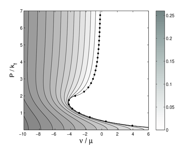
Figure 3: Contours of molecular population under various combinations of molecular centre-of-mass momentum $P$ and detuning $\nu$. The uppermost contour identifies the detuning at which bound molecules first appear for a given momentum $P$. Numbers indicate contours with a equal molecule fraction. The dots represent the result obtained analytically for the critical detuning, Eq. (16).

Figure 3 thus shows that: i) molecules are still stable for a continuum of positive detuning when $P$ is small; ii) molecules that would have been stable at negative detuning may not be such stable at intermediate momenta $P$ (although at small negative detuning they may possess small widths); and iii) in the limit $P\rightarrow\infty$, the borderline between stable and unstable again returns to zero detuning. Detailed information on the spectral density can also be used to elicit the momentum distribution of molecular pairs, a task that will be completed in future work Bortolotti .

Thus far, these are rigorous results, at least within the simplifying approximations made above. Once this is done, the effective dissociation energy of the molecules within the medium is determined. The relation between the molecule’s total energy at dissociation and the molecule’s momentum is then easily determined from kinematics, plus simple considerations on the Pauli blocking of the atomic fermions. For example, consider the case where the molecule’s kinetic energy is greater than twice the atomic Fermi energy, i.e., $P^{2}/2(m_{f}+m_{b})\geq 2\times k_{f}^{2}/2m$. At the same time, the molecule is assumed to be exactly at its dissociation threshold, so that it could live equally well as a molecule or as two free atoms. Upon dissociating, each atom would carry away half the energy, so in particular the fermionic atom is at the top of the Fermi sea, and this dissociation is not prevented by the Pauli exclusion principle. The total energy of the molecule at its dissociation threshold is then determined simply by the molecular kinetic energy, and no contribution is required from the molecular binding energy. Thus, if B represents the internal energy of the pairs relative to threshold, bound molecules are possible when

$$B\leq 0\;\;\;\;\;{\rm for}\;\;\;\;\;P\geq\sqrt{{2(m_{b}+m_{f})\over m_{f}}}k_{f}.$$ (12)

Alternatively, suppose the molecules have less than twice the atomic Fermi energy, $P^{2}/2(m_{f}+m_{b})\leq 2\times k_{f}^{2}/2m$. Now it is no longer guaranteed that the molecules can automatically decay in the many-body environment, since the fermion’s kinetic energy may lie below the Fermi level of the atomic gas. In such a case, the molecule can sustain a positive internal energy without dissociating, simply due to Pauli blocking. To decide how high this binding energy can be, we examine the conservation of energy and momentum in the dissociation process:

$${\bf P} = {\bf p}_{f}+{\bf p}_{b}$$ (13)

$$\frac{P^{2}}{2(2m)}+B = \frac{p_{b}^{2}}{2m_{b}}+\frac{p_{f}^{2}}{2m_{f}}.$$ (14)

Here ${\bf p}_{f}$, ${\bf p}_{b}$, and ${\bf P}$ are the momenta of the atomic fermions, atomic bosons, and molecules, respectively. To ensure that the atomic fermion emerges with the maximum possible kinetic energy, we consider the case where ${\bf P}$ and ${\bf p}_{f}$ point in the same direction. To ensure that $p_{f}>k_{f}$, where $k_{f}$ is the atomic Fermi momentum, along with (14), implies that molecules are stable when

$$B\leq{(m_{f}P-(m_{b}+m_{f})k_{f})^{2}\over 2m_{b}\ m_{f}(m_{b}+m_{f})}\;\;\;\;\;{\rm for}\;\;\;\;\;P\leq\sqrt{{2(m_{b}+m_{f})\over m_{f}}}k_{f}.$$ (15)

Figure 4 shows the internal energy of the molecules evaluated at the stability boundary, as described above, as a function of centre of mass momentum. The solid line in this figure is determined numerically from the $Z=0$ contour of Fig. 3. Subtracting the kinetic energy contribution and chemical potential from the pole of the T-matrix evaluated on the contour, we obtain the molecular internal energy. Also shown, as dots, are the kinematic estimates (12,15).

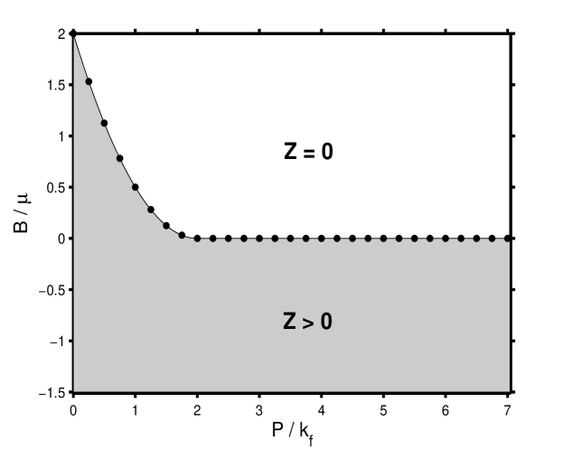
Figure 4: The internal energy that a molecule of centre-of-mass momentum $P/k_{f}$ would require to overcome Pauli blocking and dissociate. The shaded area represents numerical calculations, and the dots represent the analytical kinematic arguments in Eqs. (12,15).

Analytical expressions for the detuning at the boundary as a function of centre of mass momentum, plotted as dots in Fig. 3, are readily obtainable analytically, with similar accuracy by inspecting the denominator of Eq. (7). The total energy of the molecule, measured from the chemical potential, is, in fact, given by the pole of (7). In general this energy can be written as $E_{0}={P^{2}\over 2(m_{f}+m_{b})}-\mu+B$, where B is a complicated function of all the parameters. However, since $E_{tot}$ is a pole of (7), then $E_{0}={P^{2}\over 2(m_{f}+m_{b})}-\mu+\nu+\Pi(E_{0},P)$, so

$$\nu_{crit}=B-\Pi\left({P^{2}\over 2(m_{f}+m_{b})}-\mu+B,P\right).$$ (16)

Plugging the stability boundary value of B from Eqs. (12,15) into this formula leads to an analytic, albeit complicated, expression for the critical detuning as a function of centre of mass momentum.

IV Conclusions

The constitution and stability of a composite fermion in the many-body environment is an important part of the BF crossover regime. Within our approach we have addressed properties of strongly correlated BF pairs and defined the stability region. We concluded that in the many-body environment, low momentum molecules can be stabilized at positive detuning, and intermediate-momentum molecules can be de-stabilized, existing for shorter times at small negative detunings. We also concluded that there is always a probability to observe molecules at positive detunings, provided their momenta are less than $\approx 2p_{f}$, even though these molecules would not exist as two-body objects. The way in which these molecules are distributed will form the basis of future work.

- (1) M.Greiner,C.A.Regal, and D.S.Jin, Nature 426 , 537 (2003).
- (2) C.A.Regal, M.Greiner, and D.S.Jin, Phys.Rev.Lett. 92, 040403 (2004).
- (3) M.W.Zwierlien et al., Phys.Rev.Lett. 92, 120403 (2004).
- (4) M.Bartenstein et al., Phys.Rev.Lett. 92, 120401 (2004).
- (5) E.A. Donley et al., Nature 426, 295 (2001)
- (6) S.Inouye,J.Goldvin,M.L.Olsen,C.Ticknor,J.L.Bohn, and D.S.Jin, Phys.Rev.Lett. 93, 183201 (2004).
- (7) G. Modugno, G.Roati, F.Riboli,F.Ferliano, R.J.Brecha, M.Inguscio , Science 297 ,2240(2002)
- (8) A.Simoni, F.Ferliano, G.Roati,G.Modugno and M.Inguscio, Phys.Rev.Lett. 90, 163202 (2003)
- (9) F.Ferliano et al., cond-mat/0510630
- (10) A.Perali, A.Pieri and G.C.Strinati,Phys.Rev.Lett. 93, 100404 (2004); Phys.Rev.Lett. 95, 010400 (2005)
- (11) A.Avdeenkov and J.L.Bohn, Phys.Rev.A 71, 023609(2005)
- (12) R.B.Diener and T.L.Ho, con-mat/0404517
- (13) M.Yu.Kagan, I.V.Brofsky, D.V.Efremov, and A.V.Klaptsov, JETP 99, 640 (2004)
- (14) F.Matera , Phys.Rev.A, 68, 043624 (2003)
- (15) M.J.Bijlsma, B.A.Heringa and H.T.C.Stoof, Phys.Rev.A, 61, 053601 (2000)
- (16) K. Mlmer, Phys. Rev. Lett. 80, 1804 (1998).
- (17) M. Amoruso, A. Minguzzi, S. Stringari, M. P. Tosi, and L. Vichi, Euro. Phys. J. D 4, 261 (1998).
- (18) M.A.Baranov, L.Dobrec, and M.Lewenstein, cond-mat/0409150.
- (19) L.D.Landau and E.M.Lifshitz,Quantum Mechanics,(Butterworth-Heinemann, Oxford,UK,1981)
- (20) J.Stajic et al.,Phys.Rev.A 63, 063610 (2004)
- (21) G.M.Bruun and C.J.Pethick, Phys.Rev.Lett., 92, 140404 (2004)
- (22) H.Heiselberg, C.J.Pethic,H.Smith, and L.Viverit, Phys.Rev.Lett., 85, 2418 (2000)
- (23) A.V.Andreev,V.Gurarie, and L.Radzihovsky, Phys.Rev.Lett. 93, 130402 (2004)
- (24) A.P.Albus et al., Phys.Rev.A 65, 053607(2002)
- (25) Y. Ohashi and A. Griffin Phys. Rev. A 67, 033603 (2003).
- (26) S. J. J. M. F. Kokkelmans, J. N. Milstein, M. L. Chiofalo, R. Walser, and M. J. Holland , Phys. Rev. A 65, 053617 (2002)
- (27) R.A. Duine, H.T.C. Stoof, Phys. Rep. 396, 115 (2004).
- (28) R.G.Newton Scattering Theory of waves and particles,Second ed., Springer-Verlag, 1982
- (29) D.C.E. Bortolotti, unpublished.
- (30) D.C.E. Bortolotti, A.V. Avdeenkov, C.Ticknor, and J.L. Bohn, J. Phys B 39, 189 (2005)
- (31) A. L. Fetter and J. D. Walecka ,Quantum Theory of Many-Particles systems Dover Publications, Inc. Mineola, NY (2003)
- (32) G. D. Mahan Many-Particle Physics, III ed. Kluwer Academic/Plenum Publishers, NY (2000)