Magnetic Field Control of Exchange and Noise Immunity in Double Quantum Dots

Abstract

We employ density functional calculated eigenstates as a basis for exact diagonalization studies of semiconductor double quantum dots, with two electrons, through the transition from the symmetric bias regime to the regime where both electrons occupy the same dot. We calculate the singlet-triplet splitting $J(\varepsilon)$ as a function of bias detuning $\varepsilon$ and explain its functional shape with a simple, double anti-crossing model. A voltage noise suppression “sweet spot,” where $dJ(\varepsilon)/d\varepsilon=0$ with nonzero $J(\varepsilon)$, is predicted and shown to be tunable with a magnetic field $B$.

The goals of computation and information processing at the quantum level have stimulated the efforts of many researchers to coherently manipulate a variety of elementary quantum systems. The scope of these candidate systems is wide wide . Advanced fabrication technology and inherent scalability, however, make semiconductor systems especially promising. The investigation of these systems has recently produced some auspicious results Petta05 ; Hanson05 ; Johnson05 ; Hatano05 ; Elzerman04 . The goal of these particular studies is to coherently manipulate and probe the spin and charge state of a small (typically electron number $N$=1 or 2) system using: (i) time-varying electric fields from pulsed gates; (ii) charge sensors from nearby quantum point contacts (QPCs) Elzerman03 ; Field93 ; and (iii) externally applied magnetic fields $B$. Attention has focused recently on the regime adjacent to the degeneracy line between the double dot charge states ($N_{L}$, $N_{R}$) = (1,1) and (0,2) Petta05 . Here $N_{L}$ and $N_{R}$ denote the electron numbers on the left and right dots.

In Ref. Petta05 the lateral gates confining the double dot were pulsed to produce a controllable “detuning” $\varepsilon$ of the potential ($\varepsilon$ is the potential difference between left and right gates measured from the degeneracy point of (1,1) and (0,2)), in order to first prepare two electrons in a singlet state in one (say, the right) dot, separate them into the two dots, and then recombine them in the right dot, i.e., $(0,2)\rightarrow(1,1)\rightarrow(0,2)$. For the employed gate voltages and dot level spacings, the recombination was suppressed by Pauli blocking in the case where the (1,1) electron is in a triplet Ono02 . The singlet-triplet splitting, or exchange coupling $J(\varepsilon)$, the spin phase coherence time and the damping of Rabi oscillations between singlet and triplet were all thereby measured as functions of $\varepsilon$ at the separation point, the inter-dot tunnel coupling $t$, and magnetic field $B$. As $\varepsilon\rightarrow 0^{-}$, $J(\varepsilon)$ exhibited a rapid rise such that $dJ/d\varepsilon$ increased with $J$. The effect of large $dJ/d\varepsilon$ is to enhance sensitivity to voltage noise. The damping of Rabi oscillations, whose frequency is determined by $J(\varepsilon)$, appeared to increase with frequency, presumably due to dephasing caused by this voltage noise.

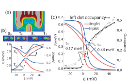
Figure 1: (a) Self-consistent effective 2D potential profile at 2DEG level, gate pattern superimposed; (b) Lowest two singlet and triplet CI energies and difference of lowest triplet and singlet $J$ (triangles, right axis) versus detuning $\varepsilon$, upper panel of (b) shows density of four states at $\varepsilon=-18\,mV$(dots indicated) with $S_{0}$ and $T_{0}$ delocalized and $S_{1}$ and $T_{1}$ mostly in right dot; (c) $J(\varepsilon)$ for two (singlet) tunnel coupling strengths $t$ (triangles and boxes) and lowest singlet and triplet occupancies of left dot (right axis) for each $t$.

In this Letter we identify ranges of parameters where a noise-immunity “sweet spot” in exchange can be found, that is, where exchange is present ($|J(\varepsilon)|>0$) but the system is insensitive to first order electrical noise ($\partial J/\partial\varepsilon=0$). The sweet spot is identified in configuration interaction (CI) calculations Stopa05 for the electronic structure of the double quantum dot with $N=2$ in Ref. Petta05 . The CI calculation employs basis states computed with density functional theory (DFT) Stopa96 to obtain full geometric fidelity to the experimental structure. We calculate $J(\varepsilon)$ from the symmetric limit at the center of the (1,1) honeycomb in the stability diagram well into the (0,2) regime with both electrons on a single dot. Analysis within a Hartree-Fock (HF), double anti-crossing model allows us to deduce simple expressions in the control parameters by which the noise-immune regime can be accessed Hu06 .

DFT calculations for lateral heterostructures have been described extensively in the literature Stopa96 . We correct the DFT single particle energies of the N=2 double dot to avoid double counting of the Coulomb interaction which is diagonalized in the basis of Kohn-Sham states $\phi_{i}$ Stopa05 . The advantage of this method is that the basis itself varies with gate voltages and $B$ and thereby captures much of the evolving structure, much as a natural basis does in quantum chemistry natural ; Fulde . The basis states are states of the full double dot and so no artificial tunneling coefficient needs to be incorporated tunneling . Finally, the Coulomb matrix elements automatically include screening by the electrical environment and can be calculated very efficiently with the kernel of Poisson’s equation, which is a natural byproduct of the DFT calculation.

The self-consistent potential profile from the DFT calculation, with the device gate pattern superimposed, is shown in Fig. 1(a). Here, the bias is approximately symmetric and the potential minima of the two dots ($\sim 5\,meV$ below the Fermi surface) are nearly equal. Figure 1(b) displays the CI-calculated lowest two singlet (S) and triplet (T) eigenstates as a function of $\varepsilon$. The singlet and triplet ground states each anti-cross with their corresponding first excited states (the calculation preserves total spin). Also plotted is $J(\varepsilon)\equiv E_{T}^{-}-E_{S}^{-}$, where $E_{T}^{-}$ and $E_{S}^{-}$ are the triplet and singlet ground states, respectively. The nature of the four anti-crossing states for $\varepsilon\approx-18\,mV$ is shown by the total (2D) density plots on the figure. Here, near the anti-crossing, the two excited states on the (1,1) side each have their densities concentrated in one dot, that is, they are the states that become S and T (0,2) ground states for $\varepsilon>0$ anticross . Fig. 1(c) exhibits $J(\varepsilon)$ for two inter-dot tunnel-coupling strengths. Also shown are the S (red) and T (blue) total occupancies of the left dot versus $\varepsilon$. The calculated results exhibit a coupling-dependent rapid increase of $J(\varepsilon)$, as experimentally observed. Additionally, in the (0,2) region ($\varepsilon>0$), where the $\varepsilon$ dependence of $J$ was not experimentally explored, the calculation predicts a saturation.

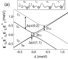
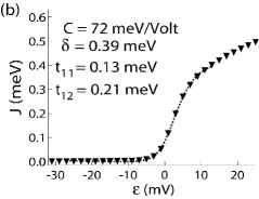
Figure 2: (a) Schematic of double anti-crossing near (1,1) to (0,2) transition. Singlets (solid) anti-cross with $t_{11}$, triplet (dashed) with $t_{12}$. Singlet-triplet splitting of ground ($\Delta_{ST}(1,1)$) and excited ($\Delta_{ST}(0,2)$) states in (1,1) region indicated. Top inset: schematic of the configurations of the four anti-crossing states. (b) Fit of calculated $J(\varepsilon)$ to anti-crossing equation 2 (dashed line) for $t=0.17\,meV$ case in Fig. 1. Triangles reproduce points in Fig. 1(c).

The structure of the numerical results in Fig. 1(b) suggest that we can explain the shape of $J(\varepsilon)$ in terms of two overlapping anti-crossings. These can be determined in their ideal form within a simple Hartree-Fock (HF) approximation where the four “bare” states are written spectroscopic as $S_{0}\equiv(L1\uparrow R1\downarrow)$, $S_{1}\equiv(R1\uparrow R1\downarrow)$ (singlets) and $T_{0}\equiv(L1\uparrow R1\uparrow)$, $T_{1}\equiv(R1\uparrow R2\uparrow)$ (triplets). The single particle energies are written $\epsilon_{R1}$, $\epsilon_{L1}$ and $\epsilon_{R2}$ (we don’t use $\epsilon_{L2}$). We include the electrostatic potentials of the dot potential minima, $eC\phi_{L}$ and $eC\phi_{R}$ in the bare level energies (here $C$ is a gate-to-dot lever arm, assumed constant) hence $\epsilon_{L1}=\epsilon_{L1}^{0}+eC\phi_{L}$, where $\epsilon_{L1}^{0}$ denotes the energy measured from the dot bottom. Similar expressions hold for the other level energies. Within a HF type description, the bare eigenfunctions are retained and the energies are shifted by direct and exchange Coulomb matrix elements. Thus we write: $E_{S}^{0}=\epsilon_{L1}+\epsilon_{R1}+V_{inter}$, $E_{S}^{1}=2\epsilon_{R1}+V_{intra}$, $E_{T}^{0}=\epsilon_{L1}+\epsilon_{R1}+V_{inter}-V_{inter}^{ex}$ and $E_{T}^{1}=\epsilon_{R1}+\epsilon_{R2}+V_{intra}-V_{intra}^{ex}$. For simplicity we here ignore the state-dependence of the inter- and intra- dot matrix elements. We also include the two (inter- and intra- dot) exchange matrix elements only in the triplet terms. The anti-crossing of the singlets results from the tunnel coupling of the two single particle ground states which we denote $t_{11}$ However, crucially, the triplets anti-cross with tunnel coupling $t_{12}$, since the $R1$ state is blocked by the Pauli principle. Due to the humped shape of the barrier, tunneling from $L1$ to the higher $R2$ is stronger ($t_{12}>t_{11}$) and this is evident in Fig. 1(b). The two branches of the singlet and triplet are found by diagonalizing the standard 2x2 determinants:

$$\begin{split}E_{S\pm}=&\tilde{E}_{S}\pm 0.5\sqrt{(C\varepsilon)^{2}+4t_{11}}\\ E_{T\pm}=&\tilde{E}_{T}\pm 0.5\sqrt{(\delta-C\varepsilon)^{2}+4t_{12}}\end{split}$$ (1)

where $\tilde{E}_{T}\equiv(E_{T}^{0}+E_{T}^{1})/2$ and $\tilde{E}_{S}\equiv(E_{S}^{0}+E_{S}^{1})/2$. As noted above, $\varepsilon$ is by definition zero at the singlet anti-crossing. In terms of the HF energies: $C\varepsilon\equiv eC(\phi_{L}-\phi_{R})-\epsilon_{R1}-\epsilon_{L1}-V_{inter}+V_{intra}=0$. Also, $\delta$ is the detuning (in units of energy, i.e. multiplied by the lever arm $C$) at which the triplet anti-crosses, relative to that of the singlet. It is given by $\delta\equiv\epsilon_{R2}^{0}-\epsilon_{R1}^{0}-V_{inter}^{ex}+V_{intra}^{ex}$. The exchange splitting is the difference between the two lower branches in 1:

$$J(\varepsilon)=\tilde{E}_{T}-\tilde{E}_{S}-0.5\sqrt{(C\varepsilon-\delta)^{2}+4t_{12}^{2}}+0.5\sqrt{(C\varepsilon)^{2}+4t_{11}^{2}}$$ (2)

note that $\tilde{E}_{T}-\tilde{E}_{S}$ is independent of $\varepsilon$.

Figure 2(a) shows the energy for the few levels, $E_{S\pm},E_{T\pm}$. Away and to the left of the anti-crossings, the gap between the ground states S and T is $E_{T}^{0}-E_{S}^{0}\equiv\Delta_{ST}(1,1)=-V_{inter}^{ex}$ theorem . The gap between the (bare) excited states is $E_{T}^{1}-E_{S}^{1}\equiv\Delta_{ST}(0,2)=\epsilon_{R2}-\epsilon_{R1}-V_{intra}^{ex}$, i.e. it depends on a single particle level spacing in dot R. Clearly, from Fig. 2(b), as $J$ increases near $\varepsilon=0$ so too does $dJ/d\varepsilon$. For spin manipulation with noise immunity it would be advantageous to find a regime where $J$ was appreciable but $dJ/d\varepsilon$ was not. This turns out to be possible. In Fig. 2(b) we also fit $J(\varepsilon)$ from Fig. 1(c) (i.e. the full CI results, specifically the curve with the smaller dot-dot coupling) with Eq. 2. The fit is good as long as points far into the (0,2) region are excluded far02 .

In what follows we show that the expression Eq. 2 has exactly one extremum, $dJ/d\varepsilon=0$, except where $t_{11}=t_{12}$. We then show in what parameter region the extremum is a minimum and how the parameters can be modulated by magnetic field $B$ to accentuate that minimum.

First, to show that $J(\varepsilon)$ has a single minimum, we take the derivative of Eq. 2:

$$\frac{dJ}{d\varepsilon}=-0.5\frac{(C\varepsilon-\delta)}{\sqrt{(C\varepsilon-\delta)^{2}+4t_{12}^{2}}}+0.5\frac{C\varepsilon}{\sqrt{(C\varepsilon)^{2}+4t_{11}^{2}}}$$ (3)

and observe that the two terms are sigmoidal curves which (for $t_{11}\neq t_{12}$) must intersect in one point, specifically $\varepsilon_{m}=\delta/(1-(t_{12}/t_{11}))$. A second derivative

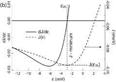
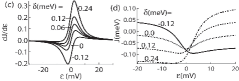
Figure 3: $dJ/d\varepsilon$ (solid, left scale) and $J(\varepsilon)$, from Eqs. 3 and 2, resp., for tunnel and $\delta$ parameters in Fig. 2(b). Note, offset energies, $\tilde{E}_{S}$ $\tilde{E}_{T}$ taken as zero throughout figure, so offsets of $J$ arbitrary. Expanded view in (b) shows minimum ($dJ(\varepsilon_{m})/d\varepsilon\equiv 0$) and depth of minimum. As $\varepsilon\rightarrow-\infty$, $J$ saturates above the figure. For same tunnel coefficients, $dJ/d\varepsilon$ (c) and $J(\varepsilon)$ (d), for a range of values of $\delta$. Minimum of $J(\varepsilon)$ (i.e. $\varepsilon_{m}$) switches sign to positive when $\delta$ changes sign to negative.

test shows that for $t_{12}>t_{11}$ (the usual case), the extremum is a minimum. Note also that, assuming $t_{12}>t_{11}$, $\delta>0\Rightarrow\varepsilon_{m}<0$ (the minimum is in the (1,1) zone) and $\delta<0\Rightarrow\varepsilon_{m}>0$.

Evaluating the depth $D$ of the minimum of $J(\varepsilon)$ yields $D\equiv J(\varepsilon_{m})-J(\varepsilon\rightarrow-\infty)=0.5\delta(1-\sqrt{1+4|t_{12}-t_{11}|^{2}/|\delta|^{2}}\approx|t_{12}-t_{11}|^{2}/|\delta|$. The full CI calculations, which include the realistic inter-dot barrier, allow us to estimate the tunnel coefficients (compare Fig. 1(b) where the singlet and triplet anti-crossings have gaps of $2t_{11}$ and $2t_{12}$, respectively). Here, and in comparable parameter ranges, the tunnel coefficient ratio $t_{12}/t_{11}\sim 1.3$. From its definition, $\delta$ is the level spacing of dot R corrected by inter- and intra-dot exchange energies and, at B=0, is of order $1.2\,meV$ from calculations for the device in Ref. Petta05 . Note that $\delta$ forms the major portion of $\Delta_{ST}(0,2)$ (cf. Fig. 2(a)) and that reducing $\Delta_{ST}(0,2)$ while keeping $\Delta_{ST}(1,1)$ relatively fixed causes the two anti-crossings to move closer to one another. For non-zero $B$ in a circular parabolic potential, the lowest branch of the $2$ state converges toward the $1$ state and the exchange term (Hund’s coupling) can induce a transition in the $N=2$ single dot to a triplet ground state; Fig. 4(a) and Ref. Tarucha . Simultaneously, $B$ induces a singlet to triplet transition in the (1,1) ground state by enhancing the wavefunction overlap in the saddle point Stopa05 ; Burkard ; Hu , but the influence on the (0,2) single particle levels is greater and the result is a drastic decrease in $\delta$, which can even become negative.

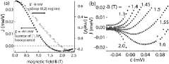
Figure 4: Magnetic field dependence of $J$, from full CI calculations, for center of (1,1) honeycomb cell (i.e. balanced gate voltages) triangles, and for strong (0,2) regime where both electrons occupy right dot, boxes. Note carefully difference between left and right scales. Single dot requires greater $B$ to drive S-T transition, but $|dJ/dB|$ is much greater in (0,2). (b) Full CI calculation for $J(\varepsilon)$ for various $B$ for strong coupling case in Fig. 1(c). Effect of $B$ is principally to reduce single particle level spacing and thereby reduce $\Delta_{ST}(0,2)$ (compare Fig. 2(a)). This moves triplet anti-crossing to lower $\varepsilon$, i.e. reduces $\delta$, simultaneously deepening the minimum of $J(\varepsilon)$. When triplet anti-crosses before the singlet ($\delta<0$, $B=1.55\,T$ and greater), the minimum of $J(\varepsilon)$ occurs in the (0,2) zone ($\varepsilon>0$).

Figure 4(b) shows $J(\varepsilon)$ computed (full CI) for a variety of $B$ values and for $t=0.46\,meV$. The minima increasingly deepen as a function of $B$ and move to larger $\varepsilon$. Note that for this large value of tunnel coupling strength the minimum for small $B$ (e.g. the $B=1.3\,T$ curve) is not observed at all. In this case the tunnel coupling is comparable in scale to the level spacing and when $\delta$ is large ($B$ is small) mixing of higher levels apparently invalidates the simple, two-level HF picture which we have used. The point is, however, that $t$ and $B$ can be varied to change the order of singlet and triplet anti-crossings ($\delta$ goes from $>0$ to $<0$). This shifts the minimum of $J(\varepsilon)$ from (1,1) to (0,2) and, for $\delta=0$ the minimum can become very deep.

In summary,we have demonstrated that device parameters can be tuned near the (1,1) to (0,2) crossover to generate a relatively noise-immune sweet spot where the exchange $J(\varepsilon)$ exhibits a minimum. The depth of the minimum, $\sim|t_{12}-t_{11}|^{2}/|\delta|$, and its detuning value, $\varepsilon_{m}=\delta/(1-(t_{12}/t_{11}))$, can be modulated with magnetic field and tunnel barrier height. The existence of this noise-immune point for spin interactions is a promising development for quantum dot quantum computation.

We acknowledge the National Nanotechnology Infrastructure Network Computation project, NNIN/C, for computational resources. We thank Edward Laird, Amir Yacoby, Jason Petta and Jacob Taylor for helpful conversations.

References

- (1) Michael A. Nielsen and Isaac L. Chuang, Quantum Computation and Quantum Information, Cambridge University Press, Cambridge, 2000; L. M. K. Vandersypen, Ph.D. Thesis, Stanford University, July 2001.
- (2) J. Petta et al., Science 309, 2184 (2005).
- (3) R. Hanson et al., Phys. Rev. Lett. 94, 196802 (2005).
- (4) A. C. Johnson et al., Nature 435, 925 (2005); F. H. L. Koppens et al., Science 309, 1346 (2005).
- (5) T. Hatano, M. Stopa and S. Tarucha, Science 309, 268 (2005); T. Hatano, M. Stopa, T. Yamaguchi, T. Ota, K. Yamada and S. Tarucha, Phys. Rev. Lett. 93, 066806 (2004).
- (6) J. M. Elzerman et al. Nature 430, 431 (2004).
- (7) J. M. Elzerman et al. Phys. Rev. B 67, 161308 (2003).
- (8) M. Field et al., Phys. Rev. Lett. 70, 1311 (1993).
- (9) K. Ono, G. D. Austing and Y. Tokura, Science 297, 1313 (2002).
- (10) W. van der Wiel, et al., New Journal of Physics 8, 28 (2006).
- (11) M. Stopa, Phys.Rev. B 54, 13767 (1996); M. Stopa, Semicond. Sci. Technol. 13, A55 (1998).
- (12) X. Hu and S. Das Sarma, Phys. Rev. Lett. 96, 100501 (2006).
- (13) P. Löwdin, Phys. Rev. 97, 1474, 1955.
- (14) P. Fulde, Electron Correlations in Molecules and Solids, (Springer, Berlin, Heidelberg 1995).
- (15) Our analytical treatment with a Hartree-Fock model does, however, employ tunnel coefficients.
- (16) Note that at the left of Fig. 1(b), which is near the center of the (1,1) stability cell, the excited S and T states become degenerate. At this point the excited states are not (0,2) states but are rather formed from orbitals above the first orbital in each dot.
- (17) We use “” and “” to denote the lowest two single particle levels localized in one or the other dot.
- (18) The bare triplet can be lower than the singlet in the approximation where tunnel coupling is ignored.
- (19) Here the potential confinement begins to change and the bare level spacing is no longer constant.
- (20) S. Sasaki et al., Nature (London) 405, 764 (2000).
- (21) G. Burkard, D. Loss, and D. P. DiVincenzo, Phy. Rev. Lett. 59, 2070(1999).
- (22) X. Hu, and S. Das Sarma, Phy. Rev. A 61, 062301(2000); M. Stopa, Physica E 10, 103 (2001).