The relation between Feynman cycles and off-diagonal long-range order

Abstract

The usual order parameter for the Bose-Einstein condensation involves the off-diagonal correlation function of Penrose and Onsager, but an alternative is Feynman’s notion of infinite cycles. We present a formula that relates both order parameters. We discuss its validity with the help of rigorous results and heuristic arguments. The conclusion is that infinite cycles do not always represent the Bose condensate.

.1 Introduction

In 1953 Feynman suggested an order parameter for the Bose-Einstein condensation of interacting systems Fey . It involves the lengths of space-time trajectories in the Feynman-Kac representation. Three years later Penrose and Onsager introduced the concept of off-diagonal long-range order PO . The latter is now accepted as the correct order parameter. Yet Feynman cycles remain actual because they are easier to deal with, and because they provide a useful microscopic heuristic Cep ; GCL ; Sch . Another order parameter that involves space-time trajectories winding in spatial directions — rather than in the imaginary time direction — is closely related to Feynman cycles; it has been used extensively in investigations of the supersolid phase, see BSZK ; SPATS and references therein.

The theory of the ideal gas has led to the expression “Bose condensate” to designate the particles that occupy the zero Fourier mode. The concept extends to interacting systems via the off-diagonal correlation function ${\boldsymbol{\sigma}}(x,y)$. The density of the Bose condensate is then

$${\boldsymbol{\rho}}_{0}=\lim_{V\to\infty}\Big{\langle}\frac{N_{0}}{V}\Big{\rangle}=\lim_{|x-y|\to\infty}{\boldsymbol{\sigma}}(x,y).$$

Feynman’s approach introduces the density of infinite cycles, ${\boldsymbol{\varrho}}(\infty)$, to be precisely defined below. The natural question is whether these densities are identical.

The links between Feynman cycles and off-diagonal long-range order were explored by Sütő, who proved that infinite cycles occur in the ideal gas below the critical temperature Suto , and that they do not occur above it Suto2 . These results were later extended to the mean-field Bose gas BCMP ; DMP . Articles Cep ; GCL ; Sch ; BSZK ; SPATS ; Suto ; Suto2 ; BCMP ; DMP all assume, or conjecture, that ${\boldsymbol{\rho}}_{0}={\boldsymbol{\varrho}}(\infty)$ in any Bose system with reasonable interactions. We will see, however, that this cannot be true in general.

The purpose of this letter is to present an explicit relation between the off-diagonal correlation function and the densities of Feynman cycles. Namely,

$${\boldsymbol{\sigma}}(x,y)=\sum_{n\;\geqslant\;1}{\boldsymbol{c}}_{n}(x-y)\,{\boldsymbol{\varrho}}(n)+{\boldsymbol{c}}_{\infty}(x-y)\,{\boldsymbol{\varrho}}(\infty).$$ (1)

Here, ${\boldsymbol{c}}_{n}(x)$ are coefficients, and ${\boldsymbol{\varrho}}(n)$ denotes the density of particles in cycles of length $n$. We expect that

$$0\;\leqslant\;{\boldsymbol{c}}_{n}(x)\;\leqslant\;1,\quad\text{and}\quad\lim_{n\to\infty}{\boldsymbol{c}}_{n}(x)={\boldsymbol{c}}_{\infty}(x),$$

for any fixed $x$. The latter statement is not obvious. Notice that the analogous statement for ${\boldsymbol{\varrho}}(n)$ is false in general: We always have $\lim_{n}{\boldsymbol{\varrho}}(n)=0$, but it is possible that ${\boldsymbol{\varrho}}(\infty)\neq 0$. In addition, we should have

$$\lim_{|x|\to\infty}{\boldsymbol{c}}_{n}(x)=0,$$ (2)

for any fixed $n$. But ${\boldsymbol{c}}_{\infty}(x)$ may converge to a strictly positive constant ${\boldsymbol{c}}$. The formula and these properties can be established in the case of the ideal gas in the canonical ensemble Uel . It is found that

$${\boldsymbol{c}}_{n}(x)=\,{\rm e}^{-x^{2}/4n\beta}\,,\quad\quad{\boldsymbol{c}}_{\infty}(x)=1,$$

and

$${\boldsymbol{\varrho}}(n)=\frac{\,{\rm e}^{\beta\mu n}\,}{(4\pi n\beta)^{d/2}},\quad\quad{\boldsymbol{\varrho}}(\infty)=\max(0,\rho-\rho_{\rm c}).$$

Here, $\mu$ is the chemical potential (that depends on the density $\rho$), and $\rho_{\rm c}$ is the critical density of the ideal gas. Notice that ${\boldsymbol{c}}=1$.

The interacting gas constitutes a formidable challenge to theoretical physicists. The sole mathematical proof about the occurrence of Bose-Einstein condensation deals with the hard-core lattice model at the symmetry point DLS ; KLS . A weakly interacting system is widely expected to display a Bose-Einstein condensation at low temperature. However, the question of whether interactions increase or decrease the critical temperature is still currently debated; the discussion in GCL illustrates this point by quoting several references that draw contradictory conclusions. In recent years progress has been made in understanding Bogolubov’s theory ZB . Remarkable results dealing with the ground state of low density systems are reviewed in LSSY .

Two results can be rigorously derived that add credence to the formula (1). First, for $\mu<0$, for any $\beta$, and for any repulsive interactions, we have

$$\lim_{|x-y|\to\infty}{\boldsymbol{\sigma}}(x,y)=0,\quad\text{and}\quad{\boldsymbol{\varrho}}(\infty)=0.$$

Second, a rigorous cluster expansion allows to establish Eq. (2) in the regime where $\mu<0$, and where $\beta$ is small with respect to the interactions. These results are proved in Uel .

In this letter we provide a heuristic discussion of interacting systems, and we will conclude that

• ${\boldsymbol{\rho}}_{0}={\boldsymbol{\varrho}}(\infty)$ when interactions are weak;

• ${\boldsymbol{\rho}}_{0}=0$, ${\boldsymbol{\varrho}}(\infty)>0$ in a crystal at sufficiently low temperature.

It is not clear whether a regime of parameters exists where the constant ${\boldsymbol{c}}$ differs from 0 and 1.

Throughout this letter, we denote finite volume expressions in plain characters, and infinite volume expressions in bold characters.

.2 Feynman-Kac expressions

In this section we introduce the relevant mathematical expressions in the Feynman-Kac representation of Bose systems. We consider a system of identical bosonic particles interacting with a pair potential. We study this system in the grand-canonical ensemble using the Feynman-Kac representation. The present discussion is necessarily brief, and we refer to Uel for a more extended mathematical description.

The grand-canonical partition function in a domain $D$ (a $d$-dimensional cube of size $L$, volume $V=L^{d}$, with periodic boundary conditions) can be expressed using the Feynman-Kac representation Gin . With $\beta$ the inverse temperature and $\mu$ the chemical potential, it is given by

$$Z=\sum_{k\;\geqslant\;1}\frac{1}{k!}\prod_{j=1}^{k}\biggl{[}\sum_{n_{j}\;\geqslant\;1}\frac{\,{\rm e}^{\beta\mu n_{j}}\,}{n_{j}}\int_{D}{\rm d}x_{j}\int{\rm d}W^{n_{j}\beta}_{x_{j}x_{j}}(\omega_{j})\\ \,{\rm e}^{-\beta U(\omega_{j})}\,\biggr{]}\prod_{1\;\leqslant\;i<j\;\leqslant\;k}\,{\rm e}^{-\beta U(\omega_{i},\omega_{j})}\,.$$ (3)

This expression is illustrated in Fig. 1. In words, the partition function involves a sum over the number $k$ of space-time cycles. For each cycle $j$, we sum over the winding number $n_{j}$; we integrate over the initial position $x_{j}$; we integrate over a Brownian trajectory $\omega_{j}$ that starts and ends at $x_{j}$, winding $n_{j}$ times around the time direction. Here, ${\rm d}W_{xy}^{\beta}(\omega)$ is the Wiener measure for a trajectory $\omega:[0,\beta]\to D$ such that $\omega(0)=x$ and $\omega(\beta)=y$. Given a trajectory $\omega$ with winding number $n$, we denote by $U(\omega)$ the interactions between its legs. That is,

$$U(\omega)=\sum_{0\;\leqslant\;i<j\;\leqslant\;n-1}\frac{1}{\beta}\int_{0}^{\beta}U\bigl{(}\omega(i\beta+s)-\omega(j\beta+s)\bigr{)}{\rm d}s.$$

Different trajectories $\omega$ and $\omega^{\prime}$ (with winding numbers $n$ and $n^{\prime}$) have interactions

$$U(\omega,\omega^{\prime})=\sum_{\begin{subarray}{c}0\;\leqslant\;i\;\leqslant\;n-1\\ 0\;\leqslant\;j\;\leqslant\;n^{\prime}-1\end{subarray}}\frac{1}{\beta}\int_{0}^{\beta}U\bigl{(}\omega(i\beta+s)-\omega^{\prime}(j\beta+s)\bigr{)}{\rm d}s.$$

In the two equations above, $U(x)$ denotes the pair interaction potential between two particles separated by a distance $|x|$. We suppose that $U(x)$ is nonnegative and spherically symmetric.

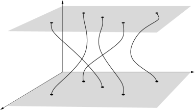
$x$$y$$\beta$$x_{1}=\omega_{1}(0)$$x_{2}=\omega_{2}(0)$$\omega_{1}(\beta)$

Figure 1: The Feynman-Kac representation of the partition function for a gas of bosons. The horizontal plane represents the $d$ spatial dimensions, and the vertical axis is the imaginary time dimension. The picture shows a situation with five particles and two cycles, with winding numbers 4 and 1.

The density of particles in cycles of length $n$ is given by the expectation of the “observable” $\frac{1}{V}\sum_{j=1}^{k}n\delta_{n_{j},n}$. Some computations yield the following finite volume expression Uel :

$$\varrho(n)=\,{\rm e}^{\beta\mu n}\,\int{\rm d}W_{00}^{n\beta}(\omega)\,{\rm e}^{-\beta U(\omega)}\,\frac{Z(\omega)}{Z}.$$ (4)

Here, $Z(\omega)$ is the grand-canonical partition function for a system where the trajectory $\omega$ is present. It is given by the same formula as Eq. (3), but with the additional term

$$\prod_{j=1}^{k}\,{\rm e}^{-\beta U(\omega,\omega_{j})}\,.$$

For repulsive interactions we always have $Z(\omega)\;\leqslant\;Z$, with equality in the ideal gas. When the volume is finite we have

$$\sum_{n\;\geqslant\;1}\varrho(n)=\Bigl{\langle}\frac{N}{V}\Bigr{\rangle}=\rho,$$

where $\rho$ is the density of the system, which depends on the chemical potential. Let ${\boldsymbol{\varrho}}(n)$ denote the thermodynamic limit of $\varrho(n)$. Limits and infinite sums do not always commute because of a possible “leak to infinity”. Fatou’s lemma garantees that

$$\sum_{n\;\geqslant\;1}{\boldsymbol{\varrho}}(n)\;\leqslant\;\rho.$$

This suggests to define the density of particles in infinite cycles by

$${\boldsymbol{\varrho}}(\infty)=\rho-\sum_{n\;\geqslant\;1}{\boldsymbol{\varrho}}(n).$$ (5)

The off-diagonal correlation function of Penrose and Onsager also has an expression in the Feynman-Kac representation. It involves an open trajectory that starts at $x$ and ends at $y$, possibly winding several times around the time direction. Precisely, we introduce

$$\sigma(x,y)=\sum_{n\;\geqslant\;1}\,{\rm e}^{\beta\mu n}\,\int{\rm d}W_{xy}^{n\beta}(\omega)\,{\rm e}^{-\beta U(\omega)}\,\frac{Z(\omega)}{Z}.$$ (6)

True to our convention we denote the thermodynamic limit by ${\boldsymbol{\sigma}}(x,y)$.

We immediately obtain a finite volume relation between $\varrho(n)$ and $\sigma(x,y)$. It is enough to consider $\sigma(0,x)$ because of translation invariance (we use periodic boundary conditions). From (4) and (6), we have

$$\sigma(0,x)=\sum_{n\;\geqslant\;1}c_{n}(x)\,\varrho(n),$$ (7)

where the coefficients $c_{n}(x)$ are given by

$$c_{n}(x)=\frac{\displaystyle\int{\rm d}W_{0x}^{n\beta}(\omega)\,{\rm e}^{-\beta U(\omega)}\,\frac{Z(\omega)}{Z}}{\displaystyle\int{\rm d}W_{00}^{n\beta}(\omega)\,{\rm e}^{-\beta U(\omega)}\,\frac{Z(\omega)}{Z}}.$$ (8)

We need to understand the thermodynamic limit of (7). “Leaks to infinity” occur, and we cannot simply replace finite volume terms by infinite volume ones. The ideal Bose gas yields exact expressions and therefore constitutes a useful first step. As $V\to\infty$, Eq. (7) becomes Uel

$${\boldsymbol{\sigma}}(0,x)=\sum_{n\;\geqslant\;1}\,{\rm e}^{-x^{2}/4n\beta}\,{\boldsymbol{\varrho}}(n)+{\boldsymbol{\varrho}}(\infty).$$ (9)

.3 Weakly interacting systems

We seek to understand the general behavior of the coefficients ${\boldsymbol{c}}_{n}$ and ${\boldsymbol{c}}_{\infty}$ in a gas of bosons with weak interactions. We can represent the numerator and denominator of (8) as the connectivity of a weakly self-avoiding random walk in a random environment. The random environment is due to $Z(\omega)$, which involves sums and integrals over configurations $\underline{\omega}$ of closed trajectories. We obtain

$$\int{\rm d}W^{n\beta}_{0x}(\omega)\,{\rm e}^{-\beta U(\omega)}\,\frac{Z(\omega)}{Z}=\int{\rm d}\nu(\underline{\omega})\,C^{\underline{\omega}}_{n}(x),$$

with $\nu$ a probability measure ($\int{\rm d}\nu(\underline{\omega})=1$), and $C^{\underline{\omega}}_{n}(x)$ the connectivity of the random walk between positions 0 and $x$:

$$C^{\underline{\omega}}_{n}(x)=\int{\rm d}W^{n\beta}_{0x}(\omega)\,{\rm e}^{-\beta U(\omega)}\,\,{\rm e}^{-\beta U(\omega,\underline{\omega})}\,.$$

The latter term represents the interactions between $\omega$ and the configuration of trajectories $\underline{\omega}$. The environment typically consists of trajectories spread all over the domain, with no significant fluctuation of density. When interactions are weak, the typical trajectory from 0 to $x$ does not depend much on the presence of the random environment. For $n$ large we have $U(\omega,\underline{\omega})\approx un$ for almost all $\omega$ and $\underline{\omega}$, where $u$ is a positive number. It is known that (weakly) self-avoiding random walks satisfy a local central limit theorem in high dimensions HHS ; BR , so that, as $n\to\infty$,

$$\frac{C^{\underline{\omega}}_{n}(x)}{C^{\underline{\omega}}_{n}(0)}\approx\exp\Bigl{(}-\frac{x^{2}}{4an\beta}\Bigr{)}.$$ (10)

The constant $a$ is greater than 1 and it reflects the (weak) self-avoidance of $\omega$. The situation is then similar to the ideal gas, and we expect the formula (1) to hold with ${\boldsymbol{c}}_{n}(x)$ given by (10), and ${\boldsymbol{c}}_{\infty}(x)=1$ for all $x$.

.4 Feynman cycles in crystals

Bosons with strong interactions are likely to undergo a usual condensation into a solid at low temperature. We consider a crystalline phase where particles display (diagonal) long-range order, and where there is no off-diagonal long-range order. (We do not consider a supersolid phase here.) We are going to argue that infinite cycles are present at very low temperature, in dimension three or more.

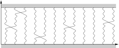
$\beta$

Figure 2: Schematic typical space-time configuration for a crystalline phase. Trajectories are roughly vertical, with occasional tunneling to a neighbor.

The typical Feynman-Kac representation for a quantum system in a crystalline phase is depicted in Fig. 2. Particles are represented by rather straight trajectories that are given by Brownian motions in the presence of an effective harmonic trap, due to the neighboring particles. Occasionally, two neighboring particles may exchange their positions through quantum tunneling. Thus Feynman cycles are associated with the following simple dynamical system. Particles occupy the sites of a lattice, and to a each bond is associated a Poisson process that exchanges the corresponding particles. The rate is proportional to $\beta$ — the actual constant depends on the potential barrier for switching two particles, and on the entropy of Brownian paths that do it. Any site belongs to a Feynman cycle of arbitrary length.

The cycle that contains a given site can also be viewed as a continuous-time discrete random walk. From time 0 to $\beta$, jumps on neighboring sites occur with a rate that is essentially independent of $\beta$. If the position at time $\beta$ is identical to the original one, the cycle closes and has winding number 1. The position is otherwise again given by a random walk, but with the following two restrictions: (a) No jump can occur if the resulting space-time picture has more than one particle at a given site; (b) if the random walk meets the other end of a bond, it has to jump in the opposite direction. (This process appears in the study Toth of the Heisenberg ferromagnet.) It is illustrated in Fig. 3. The first restriction is a self-avoidance condition; the second restriction amounts to an effective attraction. These should not be too important in dimensions higher or equal to three, where random walks are transient.

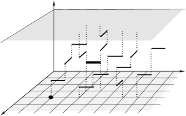
$x$$y$$\beta$

Figure 3: The Feynman cycle in a solid resembles a discrete random walk. The thick bond is crossed in both directions.

This suggests that the typical Feynman trajectories for bosons in a crystal (in 3D) is infinite if $\beta$ is large enough, and $\lim_{\beta\to\infty}{\boldsymbol{\varrho}}(\infty)=\rho$. On the other hand, the off-diagonal correlation function shows exponential decay in a crystal, and ${\boldsymbol{\rho}}_{0}=0$.

Finally, let us understand the behavior of the coefficients ${\boldsymbol{c}}_{n}(x),{\boldsymbol{c}}_{\infty}(x)$ in a crystalline phase, so as to convince ourselves that Eq. (1) and the subsequent properties are still valid. For simplicity, we assume a cubic structure, but the argument is more general. We investigate the typical space-time configurations, which contribute the most to the numerator and denominator of Eq. (8). It helps to understand first the situation without tunneling, and then to take it into account. The denominator typically involves crystalline space-time configurations as in Fig. 2. The tunneling must be such that the particle located at the origin belongs to a trajectory with winding number $n$.

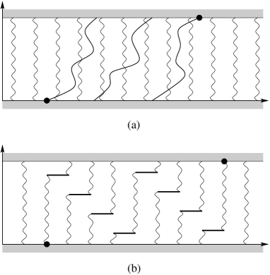
$\beta$0$x$$\beta$0$x$

Figure 4: The two possibilities for the typical open trajectory from 0 to $x$. For clarity, occasional tunneling between vertical trajectories is not shown, unlike in Fig. 2. (a) An extra trajectory is superimposed on the crystalline structure. (b) The open trajectory is part of the crystalline structure.

The numerator of (8) is more complicated. One can identify two alternative typical behavior, that are depicted in Fig. 4 (a) and (b). Both alternatives yield the same conclusion, namely that ${\boldsymbol{c}}_{n}(x)\approx\,{\rm e}^{-a|x|}\,$ provided $n$ is large (or infinite). This result should be contrasted with the weakly interacting case, where ${\boldsymbol{c}}_{n}(x)\approx 1$ if $n\gg x^{2}$.

The first alternative involves an open cycle that is superimposed to the background crystalline configuration, which is left essentially undisturbed; see Fig. 4 (a). Let $m$ be the winding number in absence of tunneling. The contribution of all trajectories is approximately

$$(4\pi\beta m)^{-d/2}\,{\rm e}^{\beta\mu^{*}m}\,\,{\rm e}^{-x^{2}/4m\beta}\,.$$ (11)

Here, $\mu^{*}=\mu-\langle U(\omega,\underline{\omega})\rangle$ is the effective chemical potential. It is negative since the crystalline phase is stable. The maximal contribution comes from $m\approx\frac{|x|}{2\beta\sqrt{-\mu^{*}}}$, and the dominant term in (11) is $\,{\rm e}^{-\sqrt{-\mu^{*}}|x|}\,$. For $n\gg|x|$ one can argue that tunneling contributes equally to the numerator and the denominator of (8), and therefore ${\boldsymbol{c}}_{n}(x)\approx\,{\rm e}^{-\sqrt{-\mu^{*}}|x|}\,$.

The second alternative is depicted in Fig. 4 (b). The open trajectory is part of the crystalline structure. Since the distance between particles is $\rho^{1/d}$, the open trajectory involves $|x|/\rho^{1/d}$ “one-directional tunnelings”. Each contributes a small factor to the ratio in (8). Since tunneling affects equally the numerator and the denominator, we again find that ${\boldsymbol{c}}_{n}(x)$ decays exponentially with $|x|$, uniformly in large $n$.

As a consequence, Eq. (1) predicts that ${\boldsymbol{\sigma}}(0,x)\to 0$ as $|x|\to\infty$, while ${\boldsymbol{\varrho}}(\infty)\neq 0$.

.5 Conclusion

We have proposed an exact relation, Eq. (1), between Feynman cycles and the off-diagonal correlation function. This relation involves the coefficients ${\boldsymbol{c}}_{n}$ which can be computed in the case of the ideal gas. It is also backed by a few rigorous results valid for interacting systems. Our study suggests that both order parameters are identical in the weakly interacting Bose gas, but not in strongly interacting systems in a crystalline phase. The density of particles in infinite cycles, ${\boldsymbol{\varrho}}(\infty)$, may be strictly positive while ${\boldsymbol{\varrho}}_{0}=0$. An interesting open question is whether ${\boldsymbol{\varrho}}(\infty)>{\boldsymbol{\varrho}}_{0}>0$ for a certain choice of parameters.

I am grateful to the referees, whose comments allowed me to improve the clarity of this letter.

References

- (1) R. P. Feynman, Phys. Rev. 91, 1291 (1953)
- (2) O. Penrose, L. Onsager, Phys. Rev. 104, 576 (1956)
- (3) D. M. Ceperley, Rev. Mod. Phys. 67, 279 (1995)
- (4) P. Grüter, D. Ceperley, F. Laloë, Phys. Rev. Lett. 79, 3549 (1997)
- (5) A. M. J. Schakel, Phys. Rev. E 63, 026115 (2001)
- (6) G. G. Batrouni, R. T. Scalettar, G. T. Zimanyi, A. P. Kampf, Phys. Rev. Lett. 74, 2527 (1995)
- (7) P. Sengupta, L. P. Pryadko, F. Alet, M. Troyer, G. Schmid, Phys. Rev. Lett. 94, 207202 (2005)
- (8) A. Sütő, J. Phys. A 26, 4689 (1993)
- (9) A. Sütő, J. Phys. A 35, 6995 (2002)
- (10) G. Benfatto, M. Cassandro, I. Merola, E. Presutti, J. Math. Phys. 46, 033303 (2005)
- (11) T. C. Dorlas, Ph. A. Martin, J. V. Pulé, J. Stat. Phys. 121, 433 (2005)
- (12) D. Ueltschi, math-ph/0605002
- (13) F. J. Dyson, E. H. Lieb, B. Simon, J. Stat. Phys. 18, 335 (1978)
- (14) T. Kennedy, E. H. Lieb, B. S. Shastry, Phys. Rev. Lett. 61, 2582 (1988)
- (15) V. A. Zagrebnov, J.-B. Bru, Phys. Reports 350, 291 (2001)
- (16) E. H. Lieb, R. Seiringer, J. P. Solovej, J. Yngvason, The mathematics of the Bose gas and its condensation, Oberwohlfach Seminars, Birkhäuser (2005)
- (17) J. Ginibre, in “Mécanique statistique et théorie quantique des champs”, Les Houches 1970, C. DeWitt and R. Stora eds, 327–427 (1971)
- (18) R. van der Hofstad, F. der Hollander, G. Slade, Probab. Th. Rel. Fields 111, 253 (1998)
- (19) E. Bolthausen, Ch. Ritzmann, math.PR/0103218
- (20) B. Tóth, Lett. Math. Phys. 28, 75 (1993)