Qubits as devices to detect the third moment of current fluctuations

Abstract

Under appropriate conditions controllable two-level systems can be used to detect the third moment of current fluctuations. We derive a Master Equation for a quantum system coupled to a bath valid to the third order in the coupling between the system and the environment. In this approximation the reduced dynamics of the quantum system depends on the frequency dependent third moment. Specializing to the case of a controllable two-level system (a qubit) and in the limit in which the splitting between the levels is much smaller than the characteristic frequency of the third moment, it is possible to show that the decay of the qubit has additional oscillations whose amplitude is directly proportional to the value of the third moment. We discuss an experimental setup where this effect can be seen.

I Introduction

A comprehensive understanding of the transport properties of mesoscopic conductors can be achieved with the study of both the average current and its fluctuations. The investigation of shot noise deJong97 ; blanter99 ; Kogan96 has proven to be a valuable tool to determine properties which are elusive to the study of current-voltage characteristics. One of the most celebrated examples in this respect is probably the measurement of the fractional charge by means of the study of shot-noise in point contacts in the Fractional Quantum Hall regime depicciotto97 ; saminadayar97 .

In the case of non-gaussian fluctuations, moments beyond the second one are relevant in characterizing the transport. In the last few years numerous theoretical studies (see Ref.delft, ) analyzed the properties of higher moments and of the full counting statistics levitov96 . In contrast to the large theoretical activity, experiments are very difficult and only few appeared so far. The first pioneering measurement of the third moment, performed by Reulet et al reulet03 , has been hindered by environmental effects beenakker03 . The first three moments of the current fluctuations in a tunnel barrier were measured very recently by Bomze et al. bomze05 confirming the Poisson statistics associated with the discreteness of the charge. Further experimental indications on the non-Gaussian character of noise were obtained by Lindell et al. lindell04 who observed its effects on a Coulomb blockade Josephson junction.

In parallel with the first experiments, and with the hope of finding more effective ways to measure higher moments, several theoretical papers appeared suggesting ways to find signatures of non-gaussian noise in the non-equilibrium properties of mesoscopic systems used as detectors. The first practical way to probe high moments of current was suggested by Lesovik in Ref.lesovik94, . In Ref.aguado, , Aguado and Kouwenhoven considered the possibility to use a double quantum dot system as detector of high frequency noise. More recently, Josephson junctions were shown to be able to act as detectors of the third heikkila04 and fourth moments of current fluctuationsankerhold05 . Their use as threshold detectors to measure the full counting statistics has been discussed by Tobiska and Nazarov tobinska04 , by Lesovik, Hassler and Blatter lesovik06 and by one of the authors pekola04 .

Qubits have been already proven very sensitive spectrometers of noise devoret00 ; astafiev04 . In this work we want to explore further the use of controllable two-level systems as noise spectrometers and analyze the possibility to employ them for the measurement of the third moment as well. With this scope in mind we derive a perturbative equation for the dynamics of two-level systems in presence of noise up to the third order in the system-noise coupling to see if, under some circumstances, we can extract some information on the third moment. In general the third order effects are masked by the dominant second order ones, since they are a result of a perturbative expansion. There are, however, situations in which the second-order correction vanishes and therefore the third order is the leading contribution. We will show that, in the usual Rotating Wave Approximation (RWA) of the system equations of motion, the contribution of the third moment is a small correction to the dominant effect of the second moment (and hence difficult to measure). A treatment beyond RWA is therefore needed and it leads to the presence of additional effects solely due to the third moment of current fluctuations.

The paper is organized as follows. In the next Section we introduce the model. We then proceed to derive the Master Equation for the reduced dynamics of the quantum system up to third order in the coupling with the environment. The reduced dynamics of the quantum system will also depend on the third-order correlations of noise and therefore it may act as a detector of these higher order moments. In Section III.1 we concentrate on the case in which the quantum system is a two-level system and show that the presence of the third order may induce coherent oscillations in the ground state population of the quantum system. Furthermore, we show that the amplitude of these oscillations is proportional to the three-point correlator of the fluctuations. In Section III.2 we discuss the case where the two-level system is subject to an external microwave field. In particular we discuss how Rabi oscillations can be influenced by the presence of the third order noise. The motivation here is to lower the frequency of the coherent oscillations into a regime which would be more accessible to experiments. Possible experimental setups where these effects can be measured are discussed in Section IV. In the same Section we analyze various complications which may emerge in the actual measurement. In particular we consider the case of a DC-SQUID as a third-moment detector. Section V is devoted to a summary of the results and possible perspectives of this approach in measuring higher order current fluctuations. Recently a similar detection scheme has been discussed in Ref.ojanen05, ; our approach is different in spirit and we will point out the difference with Ref. ojanen05, where the Rotating Wave approximation is taken for granted falci .

II Dynamics of the qubit

II.1 The model

In this first section we discuss the general formalism which will be used in the remainder of the paper. The setup under consideration is composed of a quantum system $S$ weakly interacting with a quantum bath $B$. As explained in the Introduction the quantum system will be used to investigate the properties of the bath which for example may be another nanostructure (a tunnel barrier, a point contact,…) biased at a fixed voltage and of which we want to study current fluctuations. The Hamiltonian of the total system $S+B$ can be written as follows:

$$\hat{H}_{T}=H_{S}+H_{B}+\hat{V},$$ (1)

where $H_{S}$ and $H_{B}$ are respectively the free Hamiltonian of the system and of the bath. The interaction potential, $\hat{V}$, is chosen to be of the form

$$\hat{V}=g\sum_{\alpha}\hat{N}_{\alpha}\otimes\hat{Q}_{\alpha}.$$ (2)

In the definition of $\hat{V}$, $g$ is an adimensional coupling constant and $\hat{N}_{\alpha}$ and $\hat{Q}_{\alpha}$ are operators of the bath and system respectively. The interaction is chosen to be weak so that the dynamics of the reduced density matrix of the system can be obtained by a perturbation expansion in $g$. The procedure is well known and described in various textbooks books . It is typically performed up to second order in the coupling $g$; here we do a step forward and go to the next order in the coupling. As we focus our attention on the study of the time evolution of the system $S$ in presence of a stationary bath, we have $[\rho_{B},H_{B}]=0$, $\rho_{B}$ being the bath density matrix. Moreover we assume the dynamics of the whole system to be Markovian. This means that at each order of perturbation theory we can neglect all the terms that are non-local in time.

II.2 Third order Master Equation

The time evolution of the reduced density matrix of the system in the interaction representation is described by the following third order equation (the steps leading to the master equation are standard books and we do not repeat them):

$$\dot{\rho_{I}}=Tr_{B}\left\{-\frac{g^{2}}{\hbar^{2}}\int_{0}^{\infty}\!\!dt^{\prime}\big{[}V(t),\left[V(t^{\prime}),\rho_{I}(t)\rho_{B}\right]\big{]}+\frac{ig^{3}}{\hbar^{3}}\int_{0}^{\infty}\!\!dt^{\prime}\int_{0}^{t^{\prime}}\!\!dt^{\prime\prime}\Big{[}V(t),\big{[}V(t^{\prime}),\left[V(t^{\prime\prime}),\rho_{I}(t)\rho_{B}\right]\big{]}\Big{]}\right\},$$ (3)

where we denoted respectively with $\rho_{I}$ and $V(t)$, the density matrix of the system and the interaction potential in the interaction representation. In deriving Eq.(3) we made the further assumption that $\left<V\right>=Tr_{B}[\rho_{B}V]=0$, where $Tr_{B}$ denotes the trace over the bath degrees of freedom. Taking the matrix elements of (3) between two eigenstates of the Hamiltonian of the system, after some algebra, we obtain the following third order master equation for the density matrix of $S$:

$$\dot{\rho}_{I,mn}=\sum_{kl}\rho_{I,lk}D_{knml}e^{i(E_{m}-E_{n}-E_{k}+E_{l})t},$$ (4)

where we set $H_{S}\left.|m\right>=E_{m}\left.|m\right>$, $\rho_{I,mn}=\left<m|\rho_{I}|n\right>$ and the third order relaxation matrix, $D_{knml}$, is given by the sum of two contributions:

$$D_{knml}=\frac{g^{2}}{\hbar^{2}}R_{knml}-\frac{ig^{3}}{\hbar^{3}}C_{knml}\;\;.$$ (5)

In the previous equation $R_{knml}$ is the second order relaxation matrix and $C_{knml}$ is a third order correction crucial to our treatment. Here we omit to show the explicit expression of $R_{knml}$ as it is well known and it can be found in textbooks books .
The third order kernel $C_{knml}$ can be written as follows:

$$C_{knml}=A_{knml}-A^{*}_{lmnk}+B_{mlkn}-B^{*}_{nklm},$$ (6)

with

$$A_{knml} = \sum_{\alpha\beta\gamma}\sum_{i}\left[\sum_{j}Q^{\alpha}_{mi}Q^{\beta}_{ij}Q^{\gamma}_{jl}\delta_{kn}F_{\alpha\beta\gamma}(\omega_{li},\omega_{ij})-Q^{\beta}_{mi}Q^{\gamma}_{il}Q^{\alpha}_{kn}F_{\alpha\beta\gamma}(\omega_{lm},\omega_{mi})\right]$$ (7)

$$B_{mlkn} = \sum_{\alpha\beta\gamma}\sum_{i}\left[Q^{\beta}_{ml}Q^{\gamma}_{ki}Q^{\alpha}_{in}G_{\alpha\beta\gamma}(\omega_{lm}+\omega_{ik},\omega_{ml})-Q^{\alpha}_{mi}Q^{\beta}_{il}Q^{\gamma}_{kn}G_{\alpha\beta\gamma}(\omega_{li}+\omega_{nk},\omega_{il})\right]$$ (8)

and where $\hbar\omega_{mn}=E_{m}-E_{n}$. The functions $F_{\alpha\beta\gamma}$, $G_{\alpha\beta\gamma}$ are the three-point correlators of the noise operators:

$$F_{\alpha\beta\gamma}(\omega_{1},\omega_{2}) = \int^{\infty}_{0}dt_{1}\int_{0}^{t_{1}}dt_{2}\left<N_{\alpha}(t_{1})N_{\beta}(t_{2})N_{\gamma}(0)\right>_{B}e^{i\omega_{1}t_{1}}e^{i\omega_{2}t_{2}}$$ (9)

$$G_{\alpha\beta\gamma}(\omega_{1},\omega_{2}) = \int^{\infty}_{0}dt_{1}\int_{0}^{t_{1}}dt_{2}\left<N_{\gamma}(0)N_{\alpha}(t_{1})N_{\beta}(t_{2})\right>_{B}e^{i\omega_{1}t_{1}}e^{i\omega_{2}t_{2}}\;\;.$$ (10)

We used $Q^{\alpha}_{mn}$ instead of $\left<m\,\vline\,\hat{Q}_{\alpha}\,\vline\,n\right>$, to denote the matrix elements of a system operator in the Schrödinger picture.
The average $\left<...\right>_{B}\equiv Tr_{B}[\rho_{B}...]$ is taken over the density matrix of the bath. Note that we do not need the bath to be in equilibrium but we do assume that it is stationary. An example is the noise generated by a non-equilibrium current in a voltage biased tunnel junction.

Equation (4) is quite general and many specific cases can be studied starting from it. In the Rotating Wave Approximation, i.e. neglecting oscillating terms in the sum on the right-hand side of Eq.(4), one can recover the result of Ref. ojanen05, . In this case the presence of the third order causes simply a small correction of the second order transition amplitudes and therefore it might be difficult to detect in the presence of a large background due to the second order contribution. In the following sections, we will analyze in more detail some special cases in which the effects of the third order relaxation matrix can be well characterized and distinguished from the second order. In particular, we will study how the third order contribution affects the decay and the Rabi oscillations of a two-level probe quantum system.

III Results

We now specialize to the case in which the probe is a two-level quantum system. We assume that the effective Hamiltonian of the system in the presence of noise has the form

$$\hat{H}_{eff}=-\hbar\omega_{0}\hat{\sigma}_{z}+N_{T}(t)\hat{\sigma}_{x}$$ (11)

when expressed in the eigenbasis of $S$, $N_{T}(t)$ is the noise operator and $\hat{\sigma}_{i}$ are the Pauli matrices. Moreover we make the hypothesis that the relevant frequencies of the noise source are much larger than the level splitting $\omega_{0}$. We thus neglect the frequency dependence of the third order correlators on scale up to $\omega_{0}$. Consequently in the calculation of the third order coefficients of the relaxation matrix, we set $F(\omega_{1},\omega_{2})\simeq F(0,0)$ and $G(\omega_{1},\omega_{2})\simeq G(0,0)$, if $\omega_{1},\omega_{2}\sim\omega_{0}$. In the following we will comment on these assumptions.

III.1 Relaxation in presence of non-gaussian noise

In case of a two-level system the third order master equation, Eq.(4), in the Schrödinger representation, reduces to

$$\dot{\rho}_{11} = \left(D_{1111}-D_{2112}\right)\rho_{11}+\left(D_{1112}+D_{2111}\right)\textrm{Re}[\rho_{12}]-i\left(D_{1112}-D_{2111}\right)\textrm{Im}[\rho_{12}]+D_{2112}$$ (12)

$$\dot{\rho}_{12} = \left(D_{1211}-D_{2212}\right)\rho_{11}+D_{2212}-i\left(D_{1212}-D_{2211}-i\omega_{0}\right)\textrm{Im}[\rho_{12}]+\left(D_{2211}+D_{1212}+i\omega_{0}\right)\textrm{Re}[\rho_{12}].$$ (13)

where $\hbar\omega_{0}=E_{2}-E_{1}$. The different elements of the third order relaxation matrix, $D_{knml}$, can be calculated using the definition given in the previous paragraph, Eqs. (5)-(10). Within our hypothesis, the only nonzero second order contributions are

$$D_{2112} = \frac{g^{2}}{\hbar^{2}}\int^{\infty}_{-\infty}dt^{\prime}\left<N_{T}(t^{\prime})N_{T}(0)\right>e^{i\omega_{0}t^{\prime}}=W_{21}$$ (14)

$$D_{1111} = -D_{2112}(-\omega_{0})=-W_{12}$$ (15)

$$D_{1212} = \frac{g^{2}}{\hbar^{2}}\int^{\infty}_{0}dt^{\prime}\left<\{N_{T}(t^{\prime}),N_{T}(0)\}\right>e^{i\omega_{0}t^{\prime}}$$ (16)

$$D_{2211} = -D^{*}_{1212}.$$ (17)

where we have introduced the second order transition rates, $W_{12}$ and $W_{21}$.
Note that, due to our transverse coupling assumption,the third order contribution to the previous matrix elements, Eqs. (14)-(17), is zero. The other coefficients of the relaxation matrix are of the third order in the coupling constant, $g$. In the limit of a flat spectrum all these elements can be defined as follows, using only one independent parameter

$$\!\!\!\!\!D_{1112}\!=\!D_{2212}=-i\Lambda^{(3)}\,\,\,\,\,D_{2111}\!=\!D_{1211}=i\Lambda^{(3)}$$ (18)

The third order coefficient, $\Lambda^{(3)}$, is real and it can be written a sum of time-ordered products as follows

$$\Lambda^{(3)} \!\!= \!\!\frac{g^{3}}{\hbar^{3}}\int\!dt_{1}\!\int\!dt_{2}\Big{[}\left<N_{T}(t_{1})T\left(N_{T}(t_{2})N_{T}(0)\right)\right>+$$ (19)

$$+\frac{1}{3}\left<\tilde{T}\left(N_{T}(t_{1})N_{T}(t_{2})N_{T}(0)\right)\right>\Big{]}$$

where $T$ and $\tilde{T}$ denote respectively the time-ordering and the anti-time-ordering operator.

Third moment fluctuations can be measured by measuring the probability that the system is in the ground state once it was initially prepared in the state

$$\left|\Psi(t=0)\right>=\frac{1}{\sqrt{2}}\left(\left|1\right>+\left|2\right>\right)\,.$$

Indeed the ground state population as a function of time can be easily calculated from the integration of Eqs.(12)-(13)

$$\rho_{11}(t)=\frac{W_{21}}{W_{12}+W_{21}}+e^{-(W_{12}+W_{21})t}\left[A+2B\cos(\omega_{R}t)\right].$$ (20)

In the previous equation, we have introduced the renormalized frequency

$$\omega_{R}^{2}=\omega_{0}^{2}+\omega_{0}\textrm{Im}\left[D_{1212}\right]-\frac{1}{4}(W_{12}+W_{21})^{2}$$ (21)

and the coefficients $A$ and $B$ which are defined by the following equations

$$A = \frac{1}{2}\frac{W_{12}-W_{21}}{W_{12}+W_{21}}-\frac{\Lambda^{(3)}}{2\omega_{R}}+O(g^{4})$$ (22)

$$B = \frac{\Lambda^{(3)}}{4\omega_{R}}+O(g^{4}).$$ (23)

Figure 1: Ground state population as a function of time and its Fourier transform calculated for the following values of the parameters: $W_{12}+W_{21}=\omega_{0}g^{2}$, $W_{12}-W_{21}=0.05\,\omega_{0}g^{2}$, $\Lambda^{(3)}\sim 0.3\,\omega_{0}g^{3}$, $\omega_{R}=\omega_{0}$, $g^{2}=0.1$ .

The presence of the third order, or more precisely, the presence of nonzero odd moments of noise fluctuations, induces measurable effects in the dynamics of the probe quantum system. As one can see from Eqs.(20)-(23), it induces coherent oscillations in the ground state population of amplitude proportional to the third order parameter, $\Lambda^{(3)}$.

In Fig.1 we show the ground state population as a function of time and its Fourier transform. As one can see $\rho_{11}(t)$ is given by the superposition of two terms: a damped exponential whose asymptotic value is fixed by the ratio between the two transition amplitudes, $W_{12}$ and $W_{21}$, and a damped cosine term proportional to the third moment. The structure of $\rho_{11}(t)$ can be analyzed by studying its Fourier transform (shown in Fig.1 lower panel) defined as

$$\bar{f}(\omega)=\mid\int_{-\infty}^{\infty}dt\,e^{i\omega t}\left[f(t)-f(t\!=\!\infty)\right]\mid\,\,.$$

The zero frequency peak is related to the second order non-oscillating contribution, while the smaller peak at frequency $\omega_{0}$ is a pure third order effect. In absence of third moment the time dependence of the ground state population would be simply described by a damped exponential and no third order peak would appear in the Fourier transform at $\omega=\omega_{0}$.

The assumption that the noise couples to the system only through $\sigma_{x}$ (transverse coupling) was crucial in our analysis to separate the second and the third order contributions in different elements of the relaxation matrix. This assumption can be relaxed, by introducing in the Hamiltonian a longitudinal term of the form: $V_{L}(t)=g_{L}N_{L}(t)\sigma_{z}$, provided that the two noise operators $N_{T}(t)$ and $N_{L}(t)$ can be considered as uncorrelated and that $V_{L}(t)$ is weak. In this case the final result is essentially the same except for a redefinition of order $g_{L}^{2}$ of the transition amplitudes and of the renormalized frequency, $\omega_{R}$.

III.2 Effects of a microwave field

As shown in the previous section the presence of odd moments in the current fluctuations has a distinct signature in the oscillations of the ground state population in the case of transverse coupling to the noise, Eq.(11).

However, the actual measurement of these oscillations can be very difficult as their characteristic frequency, $\omega_{R}\simeq\omega_{0}$, is typically of the order of 10 GHz and the time resolution required to follow such oscillations in detail is hardly accessible. In this Section we discuss a generalization of the the case discussed before to account for the presence of an external microwave field. Our aim is to clarify under which conditions a microwave field can shift the third order peak to a lower value fixed by the detuning frequency.

In presence of microwaves, the dynamics of the quantum system can be described by the effective hamiltonian: $\hat{H}_{eff}=H_{S}+\hat{V}+\hat{M}$. The effect of the applied field leads to the term $\hat{M}=\hat{O}\cos(\Omega t)$ where $\hat{O}$ is a system operator which, quite generally, can be expressed in the form

$$\hat{O}=\frac{\hbar}{2}\left(M_{L}\hat{\sigma}_{z}+M_{T}\hat{\sigma}_{x}\right)\,.$$ (24)

The corresponding Master Equation for a two-level quantum system in the presence of a microwave field is

$$\dot{\rho}_{11} = \left(D_{1111}-D_{2112}\right)\rho_{11}+\left(D_{1112}+D_{2111}\right)\textrm{Re}[\rho_{12}]+D_{2112}-i\big{[}D_{1112}-D_{2111}-iM_{T}\cos(\Omega t)\big{]}\textrm{Im}[\rho_{12}]$$

$$\dot{\rho}_{12} = \left[D_{1211}-D_{2212}+iM_{T}\cos(\Omega t)\right]\rho_{11}+\left[M_{L}\cos(\Omega t)-\omega_{0}-i\left(D_{1212}-D_{2211}\right)\right]\textrm{Im}[\rho_{12}]$$ (26)

$$+\left[D_{2211}+D_{1212}-i\left(M_{L}\cos(\Omega t)-\omega_{0}\right)\right]\textrm{Re}[\rho_{12}]+D_{2212}-iM_{T}\cos(\Omega t).$$

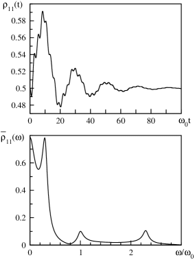
Figure 2: Ground state population as a function of time (upper panel) and its Fourier transform (lower panel) calculated in presence of a weak transverse microwave field. We chose $W_{12}=W_{21}=0.5g^{2}\omega_{0}$, $\Lambda^{(3)}=0.6\,g^{3}\omega_{0}\sim 0.002$, $\Omega=1.3\omega_{0}$, $M_{T}=0.1\omega_{0}$, and $M_{L}=0$.

Figure 3: Ground state population as a function of time (upper panel) and its Fourier transform (lower panel) calculated in presence of a strong longitudinal microwave field. The parameters are $W_{12}=W_{21}=0.5\,g^{2}\omega_{0}$, $\Lambda^{(3)}=0.3\,g^{3}\omega_{0}\sim 0.001$, $\Omega=1.3\,\omega_{0}$, $M_{L}=0.8\,\omega_{0}$, and $M_{T}=0$.

Due to the assumption of transverse coupling to the noise source and of the frequency independence of the third order correlators, the different coefficients of the third order relaxation matrix are given by Eqs.(14)-(19). Note that setting the coefficients $D_{knml}$ and the longitudinal microwave contribution $M_{L}$ to zero one easily recovers Rabi theory. In this case, solving the eigenvalue equation, one finds the known Rabi frequency: $\omega_{Rabi}=\sqrt{M_{T}^{2}/4+(\Omega-\omega)^{2}}$.

We first discuss the outcomes of a numerical integration of Eqs.(LABEL:mws1)-(26). The coupling constant and the renormalized frequency are the same in all the figures: $\omega_{R}=\omega_{0}\,\textrm{,}\,\,g^{2}=0.1$.

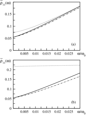
Figure 4: Amplitude of the peak at $\omega_{0}$ as a function of the third order correlator $\Lambda^{(3)}$ in absence of microwave field, (solid line), and in presence of transverse (dotted line) and longitudinal (dot-dashed line) fields. a) Weak microwave fields respectively with $M_{T}=0.1\,\omega_{0}$ or $M_{L}=0.1\omega_{0}$. b) Strong microwave fields respectively with $M_{T}=0.8\,\omega_{0}$ or $M_{L}=0.8\omega_{0}$. The other parameters are the same in both the cases: $W_{12}+W_{21}=g^{2}\omega_{0}$, $W_{12}-W_{21}=0.05\,\omega_{0}g^{2}$, $\Omega=1.3\,\omega_{0}$.

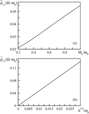
Figure 5: Amplitude of the peak at the detuning frequency $\Omega-\omega_{0}$ as a function of of the amplitude of the microwave field $M_{L}$ (a) and of the third order correlator $\Lambda^{(3)}$ (b). Values of the parameters: $W_{12}=W_{21}=0.5\,\omega_{0}g^{2}$, $\Omega=1.3\,\omega_{0}$, $M_{T}=0$. In (a) $M_{L}=0.8\,\omega_{0}$ while in (b) $\Lambda^{(3)}=0.01\,\omega_{0}$.

In Fig.2 we show $\rho_{11}(t)$ and its Fourier transform in presence of a weak transverse microwave field. The structure superimposed to the damped Rabi oscillation can be better understood by looking at the Fourier transform. We see indeed four peaks. The zero frequency peak corresponds to a pure damping term. At the detuning frequency, $\Omega-\omega_{0}$, we see a large Rabi peak whose amplitude does not essentially depend on $\Lambda^{(3)}$ and whose width is fixed by the relaxation rate $\Gamma=W_{21}+W_{12}$. At frequency $\omega_{0}$ we find the contribution arising from the third moment fluctuations which is essentially not modified by the presence of a weak transverse microwave and that depends on $\Lambda^{(3)}$ linearly. The last small peak at $\Omega+\omega_{0}$ does not originate from the third moment but is due to non-secular terms already present in second order in the coupling to the environment.

In Fig.3 we show our results in case of a strong longitudinal field. In order to suppress the second order effects, we set $W_{12}=W_{21}$; then, in the absence of third-order effects, one would simply have a constant ground state population equal to its asymptotic value $\rho_{11}(t)=\rho_{\infty}=0.5$. The non-trivial time-dependence in the ground state population is therefore completely related to the presence of the third moment fluctuations. In the case of longitudinal field in Fig.3 (lower panel), there are two peaks of non-negligible amplitude in the Fourier transform at the frequency $\omega_{0}$ and at the detuning frequency, respectively. The $\omega_{0}$ peak is the peak present also in the absence of the microwaves (both its amplitude and position are essentially not affected by the presence of the microwave field). The second peak, located at frequency $\Omega-\omega_{0}$, is a combined effect of the third moment fluctuations and of the microwave field; its amplitude is directly proportional both to the value of $\Lambda^{(3)}$ and of $M_{L}$. The position of this peak is determined solely by the detuning frequency and it is not affected by the amplitude of the microwave field, $M_{L}$.

In the case of pure longitudinal field an approximate analytical solution of Eqs.(LABEL:mws1)-(26) can be found. Up to third order in the coupling constant, $g$, we obtain

$$\rho_{11}(t) = a+be^{-(W_{12}+W_{21})t}+$$

$$+c\sum_{k=-\infty}^{\infty}J_{k}\!\left(\frac{M_{L}}{\Omega}\right)\sin\left(\left(\omega_{0}-k\Omega\right)t+\theta_{k}\right)\,\,.$$

In the previous equation $J_{k}(z)$ is the k-th Bessel function gs , the phases $\theta_{k}$ and the real constants $a$, $b$ and $c$ are defined as

$$\theta_{k} = \arctan\left(\frac{k\Omega-\omega_{0}}{W_{12}+W_{21}}\right)$$ (28)

$$a = \frac{W_{21}}{{W_{12}+W_{21}}}-\frac{\Lambda^{(3)}}{4\Omega}\!\sum_{k=-\infty}^{\infty}\!J_{k}\!\left(\frac{M_{L}}{\Omega}\right)\sin\left(\theta_{k}\right)$$ (29)

$$b = \frac{1}{2}-\frac{W_{21}}{W_{12}+W_{21}}$$ (30)

$$c = \frac{\Lambda^{(3)}}{4\Omega}$$ (31)

The peak at $\omega_{0}$ is associated to the $k=0$ contribution of the sum while the detuning frequency peak and the peak at frequency $\Omega+\omega_{0}$ are related respectively to the $k=\pm 1$ -terms. The small contribution connected with the $k=2$ Bessel function is also visible in Fig.3 at frequency $\omega=2\Omega-\omega_{0}$.

In the hope to use the method discussed in this paper for the diagnostics of the third-moment of current fluctuations it is useful to analyze the amplitudes of the different peaks in some detail. In Fig.4 the height of the peak at $\omega_{0}$ is shown as a function of $\Lambda^{(3)}$. In Fig.4a we show the results in case of weak fields. In this case, the presence of the longitudinal or the transverse field does not affect the height and the position of the third order peak. In Figure 4b we display the results in case of strong fields. As one could expect from Eqs.(LABEL:mws1)-(26), a strong transverse field masks completely the third order dependence of the $\omega_{0}$ peak; on the other hand, even a strong longitudinal microwave field does not essentially modify the height and the position of the third order peak at frequency $\omega_{0}$. Note that the range $[0,0.03]$ for $\Lambda^{(3)}/\omega_{0}$ is chosen so that the ratio between second and third order contribution varies between 0 and g.
Figures 5 and 6 are devoted to the study of the amplitude of the peak at the detuning frequency, $\Omega-\omega_{0}$, in case of pure longitudinal field. In order to compare the numerical results shown in these figures with the approximate analytical solution (LABEL:detsol), we now give the explicit expression of the $k=1$ term, which is responsible for the peak at the detuning frequency. This term can be rewritten as

$$cJ_{1}\!\left(\frac{M_{L}}{\Omega}\right)\sin\left(\Delta t+\theta_{1}\right)\simeq$$

$$\frac{\Lambda^{(3)}M_{L}}{8\Omega}\frac{(W_{12}+W_{21})\sin\left(\Delta t\right)-\Delta\cos(\Delta t)}{(W_{12}+W_{21})^{2}+\Delta^{2}}$$ (32)

where we set $\Delta=\Omega-\omega_{0}$ and in the last step we kept only the linear term in the field amplitude. In Fig.5(a) and Fig.5(b) we display the amplitude of the peak, respectively, as a function of $\Lambda^{(3)}$ and of $M_{L}$. As one could expect, the amplitude of the peak is proportional to $\Lambda^{(3)}$; moreover, as one can see in Fig.5b, the linear approximation is fulfilled also in case of strong fields. In Fig.6, we show the amplitude of the peak as a function of the detuning frequency; again the result is as expected based on Eq.(32).

Figure 6: Amplitude of the peak at the detuning frequency as a function of the $\Omega-\omega_{0}$ under longitudinal microwave coupling. Values of the parameters: $W_{12}=W_{21}=g^{2}\,\omega_{0}$, $M_{T}=0$, $M_{L}=0.8\,\omega_{0}$, $\Lambda^{(3)}=0.01\,\omega_{0}$. The inset is a magnification in the region $\Omega\simeq\omega_{0}$.

IV Experimental considerations

Starting from the results presented in the previous sections, we would like to discuss an experimental protocol for the measurement of third order noise using a two-level probe quantum system. The experimental realization of this kind of measurements is rather delicate. The basic reasons for this is that a set of inequalities has to be satisfied. First, the level spacing has to exceed the temperature in the experiment, $T$, in order to avoid thermal excitations: $\hbar\omega_{0}\gg k_{B}T$. Second, the time resolution in the experiment, $\delta t$, has to be good enough to follow the detuned coherent oscillations at angular frequency $\Omega-\omega_{0}$, i.e., $\delta t\ll|\Omega-\omega_{0}|^{-1}$. Yet the oscillation in the ground state population has to be measurable, which means that $|(\Omega-\omega_{0})/\omega_{0}|$ should not be too close to zero. This condition is determined by the resolution in measuring the population variations: for very small $|(\Omega-\omega_{0})/\omega_{0}|$, $\tilde{P}_{0}(\Omega-\omega_{0})$ is significantly suppressed as demonstrated in Fig. 6. Collecting these conditions we have

$$|(\Omega-\omega_{0})/\omega_{0}|\ll\frac{1}{\omega_{0}\delta t}\ll\frac{\hbar}{k_{B}T\delta t}.$$ (33)

As to a concrete realization, one may employ a hysteretic DC-SQUID in the tunnelling regime claudon04 . The strength of the method lies in the high contrast in resolving level occupations: tunnelling rate from the excited state is typically two to three orders higher from the excited state as compared to that from the ground state. Measurement of this decay is straightforward by observing the switching statistics, i.e., the measurement is typically repetitive in nature. Occupation probabilities of order 0.1 or even below are measurable with adiabatic detection pulses of $\delta t\sim 1$ ns duration. Measurements are typically carried out at $T\simeq 30$ mK. Taking this temperature, the condition at the right end of Eq. (33) then states that $\omega_{0}\gg 3\cdot 10^{9}$ s^-1. Typical level separations (plasma frequencies) of Josephson junctions are in the range 1 GHz $<\omega_{0}/2\pi<$ 100 GHz; thus these values are compatible with the operation temperature. With $\omega_{0}\sim 10^{10}$ s^-1 and $\delta t=1$ ns, we match the frequency vs. temperature condition with a margin of factor three. The other critical condition in Eq. (33), $|(\Omega-\omega_{0})/\omega_{0}|\ll(\omega_{0}\delta t)^{-1}$, can then be matched by requesting $|(\Omega-\omega_{0})/\omega_{0}|\ll 0.1$. Since the maximum of $\tilde{P}_{0}$ is obtained at $|\Omega/\omega_{0}-1|\simeq 0.05$, we notice that both the inequalities can be satisfied, although barely.

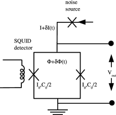
Figure 7: Schematic diagram of a possible experimental setup to detect third order fluctuations

The remaining questions then concern the coupling of the noise to the detector. As we have already pointed out, in order to see oscillations in the occupation probability due to purely third order effects, one needs to couple the noise source to $\sigma_{x}$ and the microwaves to $\sigma_{z}$. In case of a DC-SQUID detector, this means that one should couple the noise source through the current and the external microwave field through the flux. A schematic diagram of a possible measuring apparatus is shown in Fig.7. The detector is constituted by a DC-SQUID of negligible inductance formed with two identical Josephson junctions of critical current $I_{0}$ and of capacitance $C_{0}/2$ biased by external flux, $\Phi$, and current, $I$. The non-equilibrium noise source, which can be a tunnel junction or another nanostructure, induces time dependent fluctuations in the biasing current, $\delta I(t)$. Finally, the external microwave field is coupled inductively to the SQUID ring and leads to monochromatic flux fluctuations, $\delta\Phi(t)$. The effective two level hamiltonian of this system including flux and current fluctuations can be written as follows

$$H=-\frac{\hbar\omega_{p}}{2}\sigma_{z}-\hbar\omega_{p}\left[N_{T}(t)\sigma_{x}-N_{D}(t)\sigma_{z}\right]$$ (34)

The operators $N_{T}(t)$ and $N_{D}(t)$ are defined by the following equations

$$N_{T}(t) = t_{I}\frac{\delta I(t)}{I_{0}}+\left(t_{I}-2\lambda d_{\Phi}\right)\frac{\pi\delta\Phi(t)}{\Phi_{0}}$$ (35)

$$N_{D}(t) = \left(d_{\Phi}+2\lambda t_{\Phi}\right)\frac{\pi\delta\Phi(t)}{\Phi_{0}}+2\lambda t_{I}\frac{\delta I(t)}{I_{0}}$$ (36)

where $\Phi_{0}$ is the elementary flux quantum. In the previous equations we denoted with $\lambda$ and $\omega_{p}$, respectively, the SQUID anharmonicity and the SQUID plasma frequency:

$$\lambda=\frac{\eta}{6}\frac{I}{I_{c}}\left(1-\frac{I^{2}}{I_{c}^{2}}\right)^{-\frac{5}{8}}\quad\omega_{p}^{2}=\frac{2\pi}{\Phi_{0}C_{0}}\sqrt{I_{c}^{2}-I^{2}}$$ (37)

with $I_{c}=2I_{0}\cos\frac{\pi\Phi}{\Phi_{0}}$ and $\eta=\hbar^{\frac{1}{2}}(C_{0}I_{c})^{-\frac{1}{4}}\left(\frac{\Phi_{0}}{2\pi}\right)^{-\frac{3}{4}}$.
Moreover we have introduced the adimensional parameters $t_{I},\,t_{\Phi},\,d_{\Phi}$:

$$t_{I}=\frac{1}{\eta}\frac{I_{0}}{I_{c}}\left(1-\frac{I^{2}}{I_{c}^{2}}\right)^{-\frac{3}{8}}\!\!\!\!\!\!,\,\,t_{\Phi}=\frac{I}{I_{0}}t_{I}\tan\frac{\pi\Phi}{\Phi_{0}},\,\,d_{\Phi}=\tan\frac{\pi\Phi}{\Phi_{0}}\,.$$ (38)

As it is clear from Eqs.(34)-(38) a transverse coupling to current fluctuations and a longitudinal coupling to flux fluctuations (i.e. to the microwave field), can be simultaneously realized only in case of zero or very small DC component of the external biasing current. Experimentally this condition could be obtained subtracting the DC component of $I(t)$ by means of a superconducting line, as it was shown in Ref.pekola2, . In this case the SQUID potential becomes harmonic and one should also take into account the possibility to have transitions to higher levels. Anyway, if initially only the first two levels are occupied, this effect is of order higher than the third in the system-noise coupling $g$.
Assuming that the transverse coupling condition is fulfilled, that is $I<<I_{c}$, we now evaluate the amplitude of the third order oscillations for the detector’s scheme presented in Fig.7.
Comparing Eq.(34)-(38) to the model hamiltonian in Eq.(11) and using the definition given in equation (19), we rewrite $\Lambda^{(3)}$ as follows

$$\Lambda^{(3)} \!\!= \!\!\left(\frac{\omega_{p}}{\eta I_{c}}\right)^{3}\!\!\!\int\!dt_{1}\!\int\!dt_{2}\Big{[}\left<\delta I(t_{1})T\left(\delta I(t_{2})\delta I(0)\right)\right>+$$ (39)

$$+\frac{1}{3}\left<\tilde{T}\left(\delta I(t_{1})\delta I(t_{2})\delta I(0)\right)\right>\Big{]}.$$

Using the results derived by Salo, Hekking and Pekola in Ref.salo, within the framework of scattering theoryblanter99 , we can easily obtain an explicit expression of $\Lambda^{(3)}$ in terms of the transmission eigenvalues, $T_{n}$, and of the voltage bias, $V$, across the junction.
In particular, in case of energy independent scattering in the limit of zero temperature of the noise source, we have

$$\Lambda^{(3)}=\frac{4}{3}\left(\frac{e\omega_{p}}{\eta I_{c}}\right)^{3}\frac{eV}{h}\sum_{n}\,T_{n}(1-T_{n})(1-2T_{n})\,;$$ (40)

as one can see, in this limit, $\Lambda^{(3)}$ is proportional to the usual third cumulant of current statisticslevitov96 ; levitov04 . Eventually, using Eq.(40), we can also check the validity of the perturbative hypothesis and give a rough estimate of the ratio between the third and the second order contributions to the qubit dynamics. In the limit of zero frequency and zero temperature we have:

$$\frac{\Lambda^{(3)}}{W_{21}}\sim\frac{2}{3}\tilde{g}\frac{F_{3}}{F_{2}}$$ (41)

where $\tilde{g}=e\omega_{p}/(\eta I_{c})\simeq(C_{0}\,I_{c})^{-\frac{1}{4}}\cdot(2.1\,\,\,10^{-6}(A\cdot\textrm{farad})^{\frac{1}{4}})$ is an adimensional coupling constant and $F_{2}$ and $F_{3}$ are the Fano factors of the second and of the third order: $F_{2}=\sum_{n}T_{n}(1-T_{n})/\sum_{n}T_{n}$ and $F_{3}=\sum_{n}T_{n}(1-T_{n})(1-2T_{n})/\sum_{n}T_{n}$. In deriving Eq. (41) the well-known relation between the second order transition amplitude and the the Fano factor $F_{2}$ has been used, see, for example, Refs.deJong97, ; aguado, .

V Conclusions

In this paper we analyzed the possibility to use solid state qubits as detectors for higher moments of current fluctuations. We showed that in some cases there are distinct features, due to the non-secular terms in the Master equation, solely related to the presence of the third moment of current fluctuations. This may be a very interesting circumstance as usually these additional effects are masked by the large background coming from the noise (second order cumulant in the fluctuations). After having derived the general form of the Master equation up to the third order in the coupling between the environment and the bath we considered in some detail a two-level system coupled to a noise source. Indeed we found that, in the presence of purely transverse noise, the population in the ground state oscillates at a frequency $\omega_{0}$ if the two-level system is initially prepared in a superposition. The difficulty of measuring these high frequency oscillations can be alleviated by applying a microwave field. In this case the oscillations associated to the third-moment are pushed down to the detuning frequency $\Omega-\omega_{0}$.

A possible experimental implementation of this scheme of detection has been discussed in Section IV. As a two-level system (the detector) we considered a DC-SQUID and discussed the range of applicability of the scheme. Combining the narrow margins in experimental parameters and the rather unfavourable coupling of noise to the detector, it is obvious that measurement of the effects predicted here is not straightforward using a DC-SQUID as a sensor. It remains to be analyzed if other controllable two-level systems (charge qubits for example) may be more suited as detectors. Nevertheless we find interesting the existence of features entirely due to the higher moments of current fluctuations.

- (1) M. J. M. de Jong, and C. W. J. Beenakker, in Mesoscopic Electron Transport, edited by L. L. Sohn, L. P. Kouwenhoven, and G. Schön (Kluwer Academic Publishers, Dordrecht, 1997).
- (2) Ya. M. Blanter, M. Buttiker, Phys. Rep. 336, 1 (2000).
- (3) S. Kogan, Electronic Noise and Fluctuations in Solids, Cambridge University Press, Cambridge, 1996.
- (4) R. de Picciotto, M. Reznikov, M. Heiblum, V. Umansky, G. Bunin, and D. Mahalu, Nature 389, 162 (1997).
- (5) L. Saminadayar, D. C. Glattli, Y. Jin, and B. Etienne, Phys. Rev. Lett 79, 2526 (1997).
- (6) Quantum Noise in Mesoscopic Physics, edited by Y.V. Nazarov, NATO Science Series in Mathematics, Physics and Chemistry (Kluwer, Dordrecht, 2003).
- (7) L.S. Levitov, H.B. Lee, and G.B. Lesovik, J. Math. Phys. 37, 4845 (1996).
- (8) B. Reulet, J. Senzier, and D. E. Prober, Phys. Rev. Lett. 91, 196601 (2003).
- (9) C.W.J. Beenakker, M. Kindermann, and Yu.V. Nazarov Phys. Rev. Lett. 90, 176802 (2003).
- (10) Yu. Bomze, G. Gershon, D. Shovkun, L. S. Levitov, and M. Reznikov, Phys. Rev. Lett. 95, 176601 (2005).
- (11) R.K. Lindell, J. Delahaye, M. A. Sillanpää, T. T. Heikkilä, E. B. Sonin, and P. J. Hakonen, Phys. Rev. Lett. 93, 197002 (2004).
- (12) G.B. Lesovik, JETP Lett., 60, 820 (1994)
- (13) R. Aguado and L.P. Kouwenhoven, Phys. Rev. Lett. 84, 1986 (2000).
- (14) T.T. Heikkilä, P. Virtanen, G. Johansson, and F.K. Wilhelm, Phys. Rev. Lett. 93, 247005 (2004).
- (15) J. Ankerhold, H. Grabert, Phys. Rev. Lett. 95, 186601 (2005).
- (16) J. Tobiska and Yu.V. Nazarov, Phys. Rev. Lett. 93, 106801 (2004).
- (17) G.B. Lesovik, F. Hassler and G. Blatter, Phys. Rev. Lett. 96, 106801 (2006).
- (18) J.P. Pekola, Phys. Rev. Lett. 93, 206601 (2004).
- (19) M. H. Devoret and R. J. Schoelkopf, Nature 406, 1039 (2000).
- (20) O. Astafiev, Yu. A. Pashkin, Y. Nakamura, T. Yamamoto, and J. S. Tsai Phys. Rev. Lett. 93, 267007 (2004)
- (21) T. Ojanen and T. T. Heikkilä, Phys. Rev. B 73, 020501(R) (2006).
- (22) Recently the effect of counter-rotating terms has been discussed for the dynamics of a Josephson qubit in: A. D’Arrigo, G. Falci, A. Mastellone, E. Paladino, Physica E 29, 297 (2005).
- (23) J. Claudon, F. Balestro, F.W.J. Hekking, and O. Buisson, Phys. Rev. Lett. 93, 187003 (2004).
- (24) H. J. Carmichael, An Open Systems Approach to Quantum Optics (Springer-Verlag, Berlin, 1993); K. Blum, Density Matrix Theory and Applications, 2 ed. (Plenum Press, New York, 1996); C. Cohen-Tannoudji, J. Dupont-Roc, and G. Grynberg, Atom-Photon interactions, (Wiley, New York, 1992).
- (25) I.S. Gradshteyn, I.M. Ryzhik, Table of Integrals, Series and Products (Academic Press, New York, 1980).
- (26) J. P. Pekola, T. E. Nieminen, M. Meschke, J. M. Kivioja, A. O. Niskanen, and J. J. Vartiainen, Phys. Rev. Lett. 95, 197004 (2005).
- (27) J. Salo, F.W.J. Hekking, J.P. Pekola, cond-mat/0605478, (2006)
- (28) L.S. Levitov and M. Reznikov, Phys. Rev. B 70, 115305 (2004).