Density Matrix Renormalization Group for Dummies
Abstract
We describe the Density Matrix Renormalization Group algorithms for time dependent and time independent Hamiltonians. This paper is a brief but comprehensive introduction to the subject for anyone willing to enter in the field or write the program source code from scratch. An open source version of the code can be found at: http://qti.sns.it/dmrg/phome.html .
The advent of information era has been opening the possibility to perform numerical simulations of quantum many-body systems, thus revealing completely new perspectives in the field of condensed matter theory. Indeed, together with the analytic approaches, numerical techniques provide a lot of information and details otherwise inaccessible. However, the simulation of a quantum mechanical system is generally a very hard task; one of the main reasons is related to the number of parameters required to represent a quantum state. This value usually grows exponentially with the number of constituents of the system,1 due to the corresponding exponential growth of the Hilbert space. This exponential scaling drastically reduces the possibility of a direct simulation of many-body quantum systems. In order to overcome this limitation, many numerical tools have been developed, such as Monte Carlo techniques2 or efficient Hamiltonian diagonalization methods, like Lanczos and Davidson procedures.3
The Density Matrix Renormalization Group (DMRG) method has been introduced by White in 1992.4,5 It was originally devised as a numerical algorithm useful for simulating ground state properties of one-dimensional quantum lattices, such as the Heisenberg model or Bose-Hubbard models; then it has also been adapted in order to simulate small two-dimensional systems.6,7 DMRG traces its roots to Wilson’s numerical Renormalization Group (RG),8 which represents the simplest way to perform a real-space renormalization of Hamiltonians. Starting from a numerical representation of some microscopic Hamiltonian in a particular basis, degrees of freedom are iteratively added, typically by increasing the size of the finite system. Then less important ones are integrated out and accounted for by modifying the original Hamiltonian. The new Hamiltonian will thus exhibit modified as well as new couplings; renormalization group approximations consist in physically motivated truncations of the set of couplings newly generated by the elimination of degrees of freedom. In this way one obtains a simplified effective Hamiltonian that should catch the essential physics of the system under study. We point out that the DMRG can also be seen as a variational method under the matrix-product-form ansatz for trial wave functions: the ground state and elementary excited states in the thermodynamic limit can be simply expressed via an ansatz form which can be explored variationally, without referencing to the renormalization construction.9 Very recently, influence from the quantum information community has led to a DMRG-like algorithm which is able to simulate the temporal evolution of one-dimensional quantum systems.10,11,12,13,14,15,16,17
Quantum information theory has also allowed to clarify the situations in which this method can be applied efficiently. Indeed, it has been shown10 that the efficiency in simulating a quantum many-body system is strictly connected to its entanglement behavior. More precisely, if the entanglement of a subsystem with respect to the whole is bounded (or grows logarithmically with its size) an efficient simulation with DMRG is possible. Up to now, it is known that ground states of one dimensional lattices (whether critical or not) satisfy this requirement, whereas in higher dimensionality it is not fulfilled as the entanglement is subject to an area law.18 On the other hand, the simulation of the time evolution of critical systems may not be efficient even in one dimensional systems as the block entanglement can grow linearly with time and block size.19,20 In a different context, it has also been shown that in a quantum computer performing an efficient quantum algorithm (Shor’s algorithm and the simulation of a quantum chaotic system) the entanglement between qubits grows faster than logarithmically.21,22 Thus, t-DMRG cannot efficiently simulate every quantum one dimensional system; nonetheless, its range of applicability is very broad and embraces very different subjects. Indeed, DMRG can be used to study condensed matter problems and to simulate many quantum information applications in 1D quantum systems as, for example, simulations of quantum information transfer,23 quantum computations,21 the effects of decoherence on a qubit24 and the entanglement properties of one dimensional critical systems.25
The aim of this review is to introduce the reader to the last development of DMRG codes, briefly but in a comprehensive way. For the sake of briefness we do not review the vast literature of papers based on DMRG techniques and we refer the interested readers to Refs. and references therein. Here we provide both the main ideas and the technicalities needed to reach a deep understanding of DMRG and allowing an interested reader to develop its own DMRG code or modify an existing one. We also provide some easy examples that can be used as testbeds for new DMRG codes.
In Sec. I we describe the basics of time independent DMRG algorithm, in Sec. II we introduce the measurement procedure (a more detailed exposition is given in Ref. and references therein). In Sec. III the time dependent DMRG algorithm is explained. Finally, in Sec. IV we provide some numerical examples, and in Sec. V we discuss some technical issues regarding the implementation of a DMRG program code. In the last section the reader can find the schemes of the DMRG algorithms, both for the static and time dependent case. Further material can be found on our website (http://qti.sns.it/dmrg/phome.html), where the t-DMRG code will be released with an open license.
I The static DMRG algorithm
As yet pointed out in the introduction, the tensorial structure of the Hilbert space of a composite system leads to an exponential growth of the resources needed for the simulation with the number of the system constituents. However, if one is interested in the ground state properties of a one-dimensional system, the number of parameters is limited for non critical systems or grows polynomially for a critical one.18 This implies that it is possible to rewrite the state of the system in a more efficient way, i.e. it can be described by using a number of coefficients which is much smaller than the dimension of the Hilbert space. Equivalently, a strategy to simulate ground state properties of a system is to consider only a relevant subset of states of the full Hilbert space. This idea is at the heart of the so called “real space blocking renormalizarion group” which we briefly describe below, and is reminiscent of the renormalization group (RG) introduced by Wilson.8
In the real space blocking RG procedure one typically begins with a small part of a quantum system (a block of size , living on an -dimensional Hilbert space), and a Hamiltonian which describes the interaction between two identical blocks. Then one projects the composite 2-block system (of size ) representation (dimension ) onto the subspace spanned by the lowest-lying energy eigenstates, thus obtaining a new truncated representation for it. Each operator is consequently projected onto the new -dimensional basis. This procedure is then iteratively repeated, until the desired system size is reached. RG was successfully applied for the Kondo problem, but fails in the description of strongly interacting systems. This failure is due to the procedure followed to increase the system size and to the criterion used to select the representative states of the renormalized block: indeed the decimation procedure of the Hilbert space is based on the assumption that the ground state of the entire system will essentially be composed of energetically low-lying states living on smaller subsystems (the forming blocks) which is not always true. A simple counter-example is given by a free particle in a box: the ground state with length has no nodes, whereas any combination of two grounds in boxes will have a node in the middle, thus resulting in higher energy.
A convenient strategy to solve the RG breakdown is the following: before choosing the states to be retained for a finite-size block, it is first embedded in some environment that mimics the thermodynamic limit of the system. This is the new key ingredient of the DMRG algorithm; the price one has to pay is a slowdown of the system growth with the number of the algorithm’s iterations: from the exponentially fast growth Wilson’s procedure to the DMRG linear growth (very recently, in the context of real-space renormalization group methods, a new scheme which recovers the exponential growth has been proposed; this is based upon a coarse-graining transformation that renormalizes the amount of entanglement of a block before its truncation27). In the following, we introduce the working principles of the DMRG, and provide a detailed description to implement it in practice (for a pedagogical introduction see for example Refs. ).
I.1 Infinite-system DMRG
Keeping in mind the main ideas of the DMRG depicted above, we now formulate the basis structure of the so called infinite-system DMRG for one-dimensional lattice systems.The typical scenario where DMRG can be used is the search for an approximate ground state of a 1D chain of neighbor interacting sites, each of them living in a Hilbert space of dimension . As in Wilson’s RG, DMRG is an iterative procedure in which the system is progressively enlarged. In the infinite system algorithm we keep enlarging the system until the ground state properties we are interested in (e.g., the ground state energy per site) have converged.
The system Hamiltonian is written as:
| (1) |
where and are coupling constants, and , and are sets of operators acting on the -th site. The index refers to the various elements of these sets. For example, in a magnetic chain these can be angular momentum operators. For simplicity we will not describe the case of position dependent couplings, since it can be easily reduced to the uniform case.
The algorithm starts with a block composed of one site (see Fig. 1a); the arguments of refer to the number of sites it embodies, and to the number of states used to describe it. From the computational point of view, a generic block is a portion of memory which contains all the information about the block: the block Hamiltonian, its basis and other operators that we will introduce later. The block Hamiltonian for includes only the local terms (i.e. local and interaction terms where only sites belonging to the block are involved). The next step consists in building the so called left enlarged block, by adding a site to the right of the previously created block. The corresponding Hamiltonian is composed by the local Hamiltonians of the block and the site, plus the interaction term:
| (2) |
The enlarged block is then coupled to a similarly constructed right enlarged block. If the system has global reflection symmetry, the right enlarged block Hamiltonian can be obtained just by reflecting the left enlarged block.30
By adding the interaction of the two enlarged blocks, a super-block Hamiltonian is then built, which describes the global system:
| (3) |
From now on, we refer to the sites and as the free sites. The matrix should finally be diagonalized in order to find the ground state , which can be rewritten in ket notation as:
| (4) |
Hereafter Latin indexes refer to blocks, while Greek indexes indicate free sites; implicit summation convention is assumed. From one evaluates the reduced density matrix of the left enlarged block, by tracing out the right enlarged block:
| (5) |
The core of the DMRG algorithm stands in the renormalization procedure of the enlarged block, which eventually consists in finding a representation in terms of a reduced basis with at most (fixed a priori) elements. This corresponds to a truncation of the Hilbert space of the enlarged block, since .31 These states are chosen to be the first eigenstates of , corresponding to the largest eigenvalues. This truncated change of basis is performed by using the rectangular matrix (where the subscripts stand for the number of sites enclosed in the input block and in the output renormalized block), whose columns, in matrix representation, are the selected eigenstates. To simplify notations, let us introduce the function , which acts on a block index and on the next free site index and gives an index of the enlarged block running from to . The output of the full renormalization procedure is a truncated enlarged block , which coincides with the new starting block for the next DMRG iteration. This consists in the new block Hamiltonian:
and in the local operators:
| (7) |
written in the new basis. These are necessary in the next step, for the construction of the interaction between the rightmost block site and the free site. The output block includes also the matrix which identifies the basis states of the new block.
It is worth to emphasize that we can increase the size of our system without increasing the number of states describing it, by iteratively operating the previously described procedure.

On the right part (b) the scheme of a complete finite-system DMRG sweep is depicted.
We now summarize the key operations needed to perform a single DMRG step. For each DMRG step the dimension of the super-block Hamiltonian goes from to , thus the simulated system size increases by sites. The infinite-system DMRG, with reflection symmetry, consists in iterating these operations:
-
1.
Start from left block , and enlarge it by adding the interaction with a single site.
-
2.
Reflect such enlarged block, in order to form the right enlarged block.
-
3.
Build the super-block from the interaction of the two enlarged blocks.
-
4.
Find the ground state of the super-block and the eigenstates of the reduced density matrix of the left enlarged block with largest eigenvalues.
-
5.
Renormalize all the relevant operators with the matrix , thus obtaining .
Notice that at each DMRG step the ground state of a chain whose length grows by two sites is found. By contrast, the number of states describing a block is always , regardless of how many sites it includes. This means that the complexity of the problem is a priori fixed by and (while is imposed by the structure of the simulated system, is a parameter which has to be appropriately set up by the user, in order to get the desired precision for the simulation; see also Sec. IV). In Sec. V we will discuss how it is possible to extract the ground state of the super-block Hamiltonian without finding its entire spectrum, by means of efficient numerical diagonalization methods, like Davidson or Lanczos algorithms.32 We stress that at each DMRG step a truncation error is introduced:
| (8) |
where are the eigenvalues of the reduced density matrix in decreasing order. The error is the weight of the eigenstates of not selected for the new block basis. In order to perform a reliable DMRG simulation, the parameter should be chosen such that remains small, as one further increases the system size. For critical 1D systems decays as a function of with a power law, while for 1D systems away from criticality it decays exponentially, thus reflecting the entanglement properties of the system in the two regimes: a critical system is more entangled, therefore more states have to be taken into account.
I.2 Finite-system DMRG
The output of the infinite-system algorithm described before is the (approximate) ground state of an “infinite” 1D chain. In other words, one increases the length of the chain by iterating DMRG steps, until a satisfactory convergence is reached. However, for many problems, infinite-system DMRG does not yield accurate results up to the wanted precision. For example, the strong physical effects of impurities or randomness in the Hamiltonian cannot be properly accounted for by infinite-system DMRG, as the total Hamiltonian is not yet known at intermediate steps. Moreover, in systems with strong magnetic fields, or close to a first order transition, one may be trapped in a metastable state favoured for small sizes (e.g., by edge effects).
Finite-system DMRG manages to eliminate such effects to a very large degree, and to reduce the error almost to the truncation error.4 The idea of the finite-system DMRG algorithm is to stop the infinite-system algorithm at some preselected super-block length , which is subsequently kept fixed. In the following DMRG steps one applies the steps of infinite-system DMRG, but only one block is increased in size while the other is shrunk, thus keeping the super-block size constant. Reduced basis transformations are carried out only for the growing block.
When the infinite-system algorithm reaches the desired system size, the system is formed by two blocks and two free sites, as shown in the first row of Fig. 1b. The convergence is then enhanced by the so called “sweep procedure”. This procedure is illustrated in the sequent rows of Fig. 1b. It consists in enlarging the left block with one site and reducing the right block correspondingly in order to keep the length fixed. In other words, after one finite-system step the system configuration is (where represents the free site). While the left block is constructed by enlarging with the usual procedure, the right block is taken from memory, as it has been built in a previous step of the infinite procedure and saved. Indeed, during the initial infinite-system algorithm one should save the matrices , the block Hamiltonians and the interaction operators for . The finite-system procedure goes on increasing the size of the left block until the length is reached. At this stage a right block with one site is constructed from scratch and the left block is obtained through the renormalization procedure. Then, the role of the left and right block are switched and the free sites start to sweep from right to left. Notice that at each step the renormalized block has to be stored in memory. During these sweeps the length of the chain does not change, thus at each step the wavefunction of the previous one can be used as a good guess for the diagonalization procedure (see Subsec. V.2 for details). At each sweep the approximation of the ground state improves. Usually two or three sweeps are sufficient to reach convergence in the energy output.
Up to now we concentrated on a single quantum state, namely the ground state. It is also possible to find an approximation to a few number of states (typically less than ): for example, the ground state and some low-excited state.4 These states are called target states. At each DMRG step, after the diagonalization, for each target state one has to calculate the corresponding reduced density matrix , by tracing the right enlarged block. Then a convex sum of these matrices with equal weights7 is performed:
| (9) |
Finally has to be diagonalized in order to find the eigenbasis and the transformation matrices . In this way the DMRG algorithm is capable of efficiently representing not only the Hilbert space “around” the ground state, but also the surroundings of the other target states. It is worth noting that targeting many states reduces the efficiency of the algorithm because a larger has to be used for obtaining the same accuracy. An alternative way could be to run as many iterations of DMRG with a single target state as many states are required.
I.3 Boundary conditions
The DMRG algorithm, as it has been depicted above, describes a system with open boundary conditions. However, from a physical point of view, periodic boundary conditions are normally highly preferable to the open ones, as surface effects are eliminated and finite-size extrapolation gives better results for smaller system sizes. In the presented form, the DMRG algorithm gives results much less precise in the case of periodic boundary conditions than for open boundary conditions.7,33,34 Nonetheless, periodic boundary conditions can be implemented by using the super-block configuration . This configuration is preferred over because the two blocks are not contiguous, thus enhancing, for typical situations, the sparseness of the matrices one has to diagonalize and therefore maintaining the same computational speed of the algorithm for open boundary conditions.5 Simulations with the standard infinite-system super-block configuration have also been performed in order to include twisted boundary conditions, thus allowing the possibility to study spin stiffness or phase sensitivity.35
II Measure of observables
Besides the energy, DMRG is also capable to extract other characteristic features of the target states, namely to measure the expectation values of a generic quantum observable . Properties of the -site system can be obtained from the wave functions of the super-block at any point of the algorithm, although the symmetric configuration (with free sites at the center of the chain) usually gives the most accurate results. The procedure is to use the wave function resulting from the diagonalization of the super-block (see the scheme in Sec.I.1, step 4), in order to evaluate expectation values.
We first concentrate on local observables , living on one single site . If one is performing the finite-system DMRG algorithm, it is possible to measure the expectation value of at the particular step inside a sweep in which is one of the two free sites. The measure is then a simple average:
| (10) |
where is the first free site. In the special cases in which the observables refer to the extreme sites ( or ), the measurement is performed when the shortest block is , following the same procedure.
It is also possible to measure an observable expectation value while performing the infinite-system algorithm. In this case there are two possibilities: either is one of the two central free sites or not. In the former case the measurement is performed as before, while in the latter one should express in the truncated DMRG basis. At each DMRG iteration the operator must be updated in the new basis using the matrix, as in Eq. (7): . The measurement is then computed as:
| (11) |
if site belongs to the left block and analogously if belongs to the right block.
For non local observables, like a correlation function , the evaluation of expectation values depends on whether and are on the same block or not. The most convenient way in order to perform such type of measurements is to use the finite-system algorithm. Let us first consider the case of nearest neighbor observables and . We can measure the expectation value when and are the two free sites. In this case the dimensions of the matrices and are simply and we do not have to store these operators in block representation. The explicit calculation of this observable is then simply:
| (12) |
In general, measures like (where and are not nearest neighbor sites) can also be evaluated. This task can be accomplished by firstly storing the block representation of and , and then by performing the measure when belongs to a block and is a free site or vice-versa. Analogously, it is possible to evaluate measures in the case when belongs to the left block, while to the right one. What should be avoided is the measure of when and belong to the same block. Indeed, in this case the block representation of evaluated through those of and separately is not correct, due to the truncation. Instead, such type of operators have to be built up as a compound object: in order to measure them, one has also to keep track of the block representation of the product throughout all the calculation, consequently slowing down the algorithm.5,7
The standard DMRG algorithm works better with open boundary conditions (see SubSec. I.3); this necessarily introduces boundary effects in the measure of observables. For example, in the case of spin chains, open boundaries cause a strong alternation in the local bond strength at the borders, which slowly decays when shifting to the center.5 In order to obtain a good description of the bulk system by using open boundary conditions, one generally has to simulate a larger system and then discard measurements on the outer sites; the number of outer sites over which measurement outcomes strongly fluctuate depends on the simulated physical system.
Finally, we stress that usually the convergence of measurements is slower than that of energy, since more finite-system DMRG sweeps are required in order to have reliable measurement outcomes (typically between five and ten). As an example, we quote the case of the one-dimensional spin 1 Bose Hubbard model,36 in which energies typically converge after 2 or 3 sweeps, while the measure of the dimerization order parameter requires at least five sweeps to converge (the convergence gets even slower when the system approaches criticality).
III Time dependent DMRG
In this section we describe an extension of the static DMRG, which incorporates real time evolution into the algorithm. Various different time-dependent simulation methods have been recently proposed,10,12,13,37 but here we restrict our attention to the algorithm introduced by White and Feiguin.13
The aim of the time-dependent DMRG algorithm (t-DMRG) is to simulate the evolution of the ground state of a nearest-neighbor one dimensional system described by a Hamiltonian , following the dynamics of a different Hamiltonian . In few words, the algorithm starts with a finite-system DMRG, in order to find an accurate approximation of the ground state of . Then the time evolution of is implemented, by using a Suzuki-Trotter decomposition38,39 for the time evolution operator .
The DMRG algorithm gives an approximation to the Hilbert subspace that better describes the state of the system. However, during the evolution the wave function changes and explores different parts of the Hilbert space. Thus, the truncated basis chosen to represent the initial state will be eventually no more accurate. This problem is solved by updating the truncated bases during the evolution. The first effort, due to Cazalilla and Marston, consists in enlarging the effective Hilbert space, by increasing , during the evolution.37 However, this method is not very efficient because if the state of the system travels sufficiently far from the initial subspace, its representation becomes not accurate, or grows too much to be handled. Another solution has been proposed in Ref. : the block basis should be updated at each temporal step, by adapting it to the instantaneous state. This can be done by repeating the DMRG renormalization procedure using the instantaneous state as the target state for the reduced density matrix.
In order to approximately evaluate the evolution operator we use a Suzuki-Trotter decomposition.38,39 The first order expansion in time is given by the formula:
| (13) |
where gives the discretization of time in small intervals , and is the interaction Hamiltonian (plus the local terms) between site and . Further decompositions at higher orders can be obtained by observing that the Hamiltonian can be divided in two addends: the first, , containing only even bonds, and the second, , containing only odd bonds. Since the terms in and commute, an even-odd expansion can be performed:
| (14) |
This coincides with a second order Trotter expansion, in which the error is proportional to . Of course, one can enhance the precision of the algorithm by using a fourth order expansion with error :40
| (15) |
where all , except , corresponding to evolution backward in time.
Nonetheless, the most serious error in a t-DMRG program remains the truncation error. A nearly perfect time evolution with a negligible Trotter error is completely worthless if the wave function is affected by a relevant truncation error. It is worth to mention that t-DMRG precision becomes poorer and poorer as time grows larger and larger, due to the accumulated truncation error at each DMRG step. This depends on , on the number of Trotter steps and, of course, on . At a certain instant of time, called the runaway time, the t-DMRG precision decreases by several order of magnitude. The runaway time increases with , but decreases with the number of Trotter steps and with . For a more detailed discussion on the t-DMRG errors and on the runaway time, see Gobert et al.41
The initial wave function can be chosen from a great variety of states. As an example, for a spin chain, a factorized state can be prepared by means of space dependent magnetic fields. In general, it is also possible to start with an initial state built up by transforming the ground state as , where are local operators. The state can be obtained by simply performing a preliminary sweep, just after the finite-system procedure, in which the operators are subsequently applied to the transforming wave function, when is a free site.13
In summary, the t-DMRG algorithm is composed by the following steps:
-
1.
Run the finite-system algorithm, in order to obtain the ground state of .
-
2.
If applicable, perform an initial transformation in order to set up the initial state .
-
3.
Keep on the finite-system procedure by performing sweeps in which at each step the operator is applied to the system state ( and are the two free sites for the current step).
-
4.
Perform the renormalization, following the finite-system algorithm, and store the matrices for the following steps.
-
5.
At each step change the state representation to the new DMRG basis using White’s state prediction transformation43 (see below).
-
6.
Repeat points 3 to 5, until a complete time evolution has been computed.
White’s state prediction transformation43 has been firstly developed in the framework of the finite-system DMRG to provide a good guess for the Davidson or Lanczos diagonalization, thus enhancing the performance of the algorithm (see Subsec. V.2 for details). Here we briefly recall how it works, and adapt it to the time-dependent part of the DMRG algorithm. At any DMRG step, one has the left block and right block description. To transform a quantum state of the system in the new basis for the next step (corresponding to the blocks and ) one uses the matrices : and . The first matrix transforms a block of length in a block of length and it has been computed in the current renormalization. The second one transforms a block of length in a block of length ; this matrix is recovered from memory, since it has been computed at a previous step. The transformed wave function then reads:
| (16) |
Assuming this operation is already implemented, the t-DMRG algorithm introduces only a slight modification: at step (i.e. when and are the two free sites), instead of the diagonalizing the super-block with the Davidson or Lanczos, one applies to the transformed wave function.

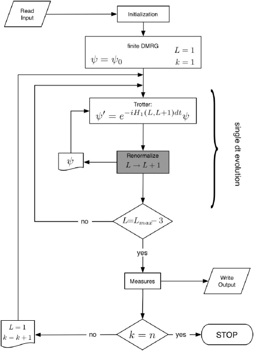
To compute the system time evolution using the first order Trotter expansion of Eq. (13), one should perform one half sweep for each time interval : at the -th step one has to apply , forming the usual left-to-right sweep. When arriving at the end of the chain, the system has been evolved of a time; one then goes on with the next time iteration, applying the corresponding evolution operators in a right-to-left sweep. Attention must be paid for the border links: at the first step both and have to be applied; an analogous situation happens at the last step. The procedure for one complete time evolution is depicted in Fig. 2. Notice that, since at each step the operator is computed on the two current free sites and (or when the block is composed of just one site), its representation is given in terms of a matrix, and most remarkably it is exact. More generally, if the border block dimension is such that it can be treated exactly, it can be convenient to perform its evolution as a whole and then switch the sweep direction. As stated before, to increase the simulation precision, one can expand the time evolution operator to the second order Trotter expansion, as in Eq. (14). The implementation of this expansion requires sweeps for each time interval : in the first is applied, in the second , finally a third half sweep is needed to apply again. In order to acquire further precision one may go to the fourth order (see Eq. (15)). In this case are needed, thus the computational time is respectively five times or fifteen times longer than the one needed by using Eq. (14) or Eq. (15).
Finally, we want to remark again that this algorithm for the time evolution is a small modification of the finite-system procedure: the main difference is the computation of a factor of the Trotter expansion instead of performing the diagonalization procedure at each step. This means that a typical t-DMRG sweep is much less time consuming that a finite-system one. Notice also that the measurements are performed in the same way as in the finite-system algorithm.
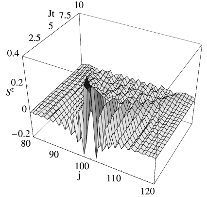
To conclude this section, we provide a simple and intuitive example which explains how the time-dependent algorithm works. We consider the time evolution of the on-site magnetization of an excited state for a spin-1 Heisenberg chain.13 In order to study the dynamics of this excitation, first we run the finite-system DMRG algorithm, thus obtaining the ground state of a -sites chain. We then perform a preliminary sweep to apply on for a single site located at the center of the chain, namely we choose . In this way we set up the initial state , that is a localized wave packet consisting of all wave vectors. We then perform the t-DMRG algorithm with being the Heisenberg hamiltonian, and instantaneously measure the local magnetization for each site : . The initial wave packet spreads out as time progresses; different components move with different speeds, given by the corresponding group velocity (see Fig. 3).
IV Numerical examples
In this section we report some numerical examples on the convergence of the DMRG outputs with respect to the user fixed parameters , and . Let us first focus on the static DMRG algorithm. The main source of error is due to the step-by-step truncation of the Hilbert space dimension of the system block from to . The parameter must be set up very carefully, since it represents the maximum number of states used to describe the system block. It is clear that, by increasing , the output becomes closer and closer to the exact solution, which is eventually reached in the limit of (in that case the algorithm would no longer perform truncation, and the only source of error would be due to inevitable numerical roundoffs). As an example of the output convergence with , in Fig. 4 we plotted the behavior of the ground state energy in the one-dimensional spin 1 Bose-Hubbard model as a function of (see Ref. for a detailed description of the physical system). The convergence is exponential with , as can be seen in the figure. In the inset the CPU-time dependence with is shown and the dashed line shows a power law fit of data, with .
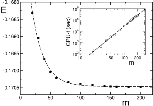
Numerical simulation presented here and in the following figures have been performed on a GHz PowerPC 970 processor with GB RAM memory.42
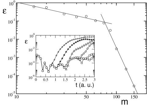
We now present an example of convergence of the t-DMRG with and . We consider the dynamical evolution of the block entanglement entropy in a linear chain (see Ref. for more details). The state of the system at time is the anti-ferromagnetic state. The initial state evolves with the Hamiltonian of the model from an initial product state to an entangled one. This entanglement can be measured by the von Neumann entropy of the reduced density matrix of the block :
| (17) |
In the example we calculate for a block of size in a chain of length . The time evolution has been calculated form to with a fixed Trotter time step that ensures that the Trotter error is negligible with respect to the truncation error.

Since the model can be solved analytically, we are able to compare the exact results with the t-DMRG data. In Fig. 5 we show as a function of time for various values of , from to , and compared with the exact data. In the inset we present the CPU-time as a function of , which behaves as a power-law with , confirming the estimate given in the inset of Fig. 4. The deviation as a function of and of time is shown in Fig. 6. The typical fast convergence of the DMRG result with is recovered only when is greater than a critical value (two distinct regimes are clear in Fig. 6). This is due to the amount of entanglement present in the system: an estimate of the number of states needed for an accurate description is given by . Thus, it is always convenient to keep track of entropy to have an initial guess for the number of states needed to describe the system.41 On the other hand, if is increased too much, the Trotter error will dominate and smaller is needed to improve accuracy.
V Technical issues
In this section we explain some technicalities regarding the implementation of DMRG and t-DMRG code. They are not essential in order to understand the algorithm, but they can be useful to anyone who wants to write a code from scratch, or to modify the existing ones. Some of these parts can be differently implemented, in part or completely skipped, depending on the computational complexity of the physical system under investigation.
V.1 Hamiltonian diagonalization
The ground state of the Hamiltonian is usually found by diagonalizing a matrix of dimensions . Typically the DMRG algorithm is used when one is only interested in the ground state properties (at most in few low-energy eigenstates). The diagonalization time can thus be greatly optimized by using Lanczos or Davidson methods: these are capable to give a small number () of eigenstates close to a previously chosen target energy in much less time than exact diagonalization routines. Moreover they are optimized for large sparse matrices, (that is the case of typical super-block Hamiltonians) and they do not require as input the full matrix. What is needed is just the effect of it on a generic state , which lives in a dimensional Hilbert space. The Hamiltonian in Eq. (1) can be written as:
| (18) |
where and act respectively on the left and on the right enlarged block. Thus, only this matrix multiplication has to be implemented:
| (19) |
In this way it is possible to save a great amount of memory and number of operations, since the dimensions of and are , and not . As an example, a reasonable value for simulating the evolution of a spin chain () is . This means that, in order to store all the complex numbers of in double precision, Gbytes of RAM is needed. Instead, each of the two matrices and requires less than kbytes of RAM.
V.2 Guess for the wave function
Even by using the tools described in the previous paragraph, the most time consuming part of a DMRG step remains the diagonalization procedure. The step-to-step wave function transformation required for the t-DMRG algorithm, which has been described in the previous section, can also be used in the finite-system DMRG, in order to speed up the super-block diagonalization.43 Indeed the Davidson or Lanczos diagonalization methods are iterative algorithms which start from a generic wave function, and then recursively modify it, until the eigenstate closest to the target eigenvalue is reached (up to some tolerance value, fixed from the user). If a very good initial guess is available for the diagonalization procedure, the number of steps required to converge to the solution can be drastically reduced and the time needed for the diagonalization can be reduced up to an order of magnitude.
In the finite-system algorithm the system is changing much less than in the infinite algorithm, and an excellent initial guess is found to be the final wave function from the previous DMRG step, after it has been written in the new basis for the current step. White’s prediction is used in order to change the basis of the previous ground state with the correct operators , as in Eq. (16). It is also possible to speed up the diagonalization in the infinite-system algorithm, but here the search for a state prediction is slightly more complicated (see, e.g., Refs. ).
V.3 Symmetries
If the system has a global reflection symmetry, it is possible to take the environment block equal to the system block, in the infinite-system procedure. Namely, the right enlarged block is simply the reflection of the left one. To avoid the complication of the reflection we can consider an alternative labelling of the sites, as shown in Fig. 7. In this case left and right enlarged blocks are represented by exactly the same matrix.

If other symmetries hold, for example conservation of angular momentum or particle number, it is possible to take advantage of them, such to considerably reduce the CPU-time for diagonalization. The idea is to rewrite the total Hamiltonian in a block diagonal form, and then separately diagonalize each of them. If one is interested in the ground state, he simply has to compare the ground state energies inside each block, in order to find the eigenstate corresponding to the lowest energy level. One may also be interested only in the ground state with given quantum numbers (for example in the Bose-Hubbard model one can fix the number of particles); in this case one has to diagonalize the block Hamiltonian corresponding to the wanted symmetry values. In order to perform this task, it is sufficient to divide the operators for the left and right block into different symmetry sectors. Then the multiplication will take into account only the sectors’ combination which preserves the total quantum number. When finding the reduced density matrix , its eigenstates have also to be symmetry-labelled. Attention must be paid when truncating to the reduced basis: it is of crucial importance to retain whole blocks of eigenstates with the same weight, inside a region with given quantum numbers. This helps in avoiding unwanted artificial symmetry breaking, apart from numerical roundoff errors.
V.4 Sparse Matrices
Operators typically involved in DMRG-like algorithms (such as block Hamiltonians, updating matrices, observables) are usually represented by sparse matrices. A well written programming code takes advantage of this fact, thus saving large amounts of CPU-time and memory. Namely, there are standard subroutines which list the position (row and column) and the value of each non null element for a given sparse matrix.
V.5 Storage
Both the static and the time dependent DMRG require to store a great number of operators: the block Hamiltonian, the updating matrices, and if necessary the observables for each possible block length. One useful way to handle all these operators is to group each of them in a register, in which one index represents the length of the block. Operatively, we store all these operators in the fast-access RAM memory. However, for very large problems one can require more than the available RAM, therefore it is necessary to store these data in the hard disk. The read/write operations from hard disk have to be carefully implemented, e.g., by performing them asyncronously, since a non optimal implementation may dramatically slow down the program performance.
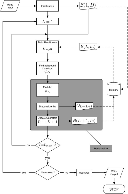
V.6 Algorithm Schemes
Acknowledgments
We thank J.J. Garcia-Ripoll and C. Kollath for some technical comments while developing the DMRG code and for feedback. We also thank G.L.G. Sleijpen32 for providing us with the Fortran routine to find the ground state. This work has been performed within the “Quantum Information” research program of Centro di Ricerca Matematica “Ennio de Giorgi” of Scuola Normale Superiore and it has been partially supported by IBM 2005 Scholars Grants – Linux on Power and by NFS through a grant from the ITAMP at Harvard University and the Smithsonian Astrophysical Observatory. SM acknowledges support from the Alexander Von Humboldt Foundation. GDC acknowledges support from the European Commission through the FP6-FET Integrated Project SCALA, CT-015714.
REFERENCES
1. R. Feynman, Int. J. Theor. Phys. 21, 467 (1982).
2. See, e.g., A Guide to Monte Carlo Simulations in Statistical Physics, D.P. Landau and K. Binder, Cambridge University Press (2000). A.W. Sandvik and J. Kurkijärvi, Phys. Rev. B 43, 5950 (1991).
3. H.A. van der Vorst, Computational Methods for large Eigenvalue Problems, in P.G. Ciarlet and J.L. Lions (eds), Handbook of Numerical Analysis, Volume VIII, North-Holland (Elsevier), Amsterdam (2002).
4. S.R. White, Phys. Rev. Lett. 69, 2863 (1992);
5. S.R. White, Phys. Rev. B 48, 10345 (1993).
6. I. Peschel, X. Wang, M. Kaulke, and K. Hallberg, eds., Density-Matrix Renormalization (Springer Verlag, Berlin, 1999).
7. U. Schollwöck, Rev. Mod. Phys. 77, 259 (2005).
8. K.G. Wilson, Rev. Mod. Phys. 47, 773 (1975).
9. S. Östlund and S. Rommer, Phys. Rev. Lett. 75, 3537 (1995).
10. G. Vidal, Phys. Rev. Lett. 91, 147902 (2003).
11. G. Vidal, Phys. Rev. Lett. 93, 040502 (2004).
12. A.J. Daley, C Kollath, U. Schollwöck, and G. Vidal, J. Stat. Mech. P04005 (2004).
13. S.R. White and A.E. Feiguin, Phys. Rev. Lett. 93, 076401 (2004).
14. A.E. Feiguin and S.R. White, Phys. Rev. B 72, 020404 (2005).
15. S.R. Manmana, A. Muramatsu, and R.M. Noack, AIP Conf. Proc. 789, 269 (2005), arXiV:cond-mat/0502396.
16. J.J. Garcia-Ripoll, New J. Phys. 8, 305 (2006).
17. U. Schollwöck and S.R. White, in G.G. Batrouni and D. Poilblanc (eds), Effective models for low-dimensional strongly correlated systems, p. 155, AIP, Melville, New York (2006).
18. G. Vidal, J.I. Latorre, E. Rico, and A. Kitaev, Phys. Rev. Lett. 90, 227902 (2003). J.I. Latorre, E. Rico, and G. Vidal, Quant. Inf. and Comp. 4, 48 (2004).
19. P. Calabrese and J. Cardy, J. Stat. Mech.: Theor. Exp. P04010 (2005).
20. G. De Chiara, S. Montangero, P. Calabrese, and R. Fazio, J. Stat. Mech.: Theor. Exp. P03001 (2006).
21. R. Orus and J.I. Latorre, Phys. Rev. A 69, 052308 (2004).
22. S. Montangero, Phys. Rev. A 70, 032311 (2004).
23. S.Bose, Phys. Rev. Lett. 91, 207901 (2003).
24. D. Rossini, T. Calarco, V. Giovannetti, S. Montangero, and R. Fazio, Phys. Rev. A 75, 032333 (2007).
25. A. Osterloh, L. Amico, G. Falci, and R. Fazio, Nature (London) 416, 608 (2002).
26. K. Hallberg, Adv. Phys. 55, 477 (2006).
27. G. Vidal, arXiV:cond-mat/0512165.
28. A.L. Malvezzi, Braz. J. of Phys. 33, 55 (2003).
29. R.M. Noack and S.R. Manmana, AIP Conf. Proc. 789, 93 (2005), arXiV:cond-mat/0510321.
30. If mirror symmetry does not hold the right enlarged block must be built up independently.
31. If is bigger than we do not truncate the basis at the first step. The truncation starts when and is the number of spins in the enlarged block.
32. To find the ground state we used the JDQZ routine implemented by D. Fokkema, G.L.G. Sleijpen, and H.A. van der Vorst http://www.math.ruu.nl/people/sleijpen/ .
33. M.C. Chung and I. Peschel, Phys. Rev. B 62, 4191 (2000).
34. F. Verstraete, D. Porras, and J.I. Cirac, Phys. Rev. Lett. 93, 227205 (2004).
35. P. Schmitteckert and U. Eckern, Phys. Rev. B 53, 15397 (1996).
36. M. Rizzi, D. Rossini, G. De Chiara, S. Montangero, and R. Fazio, Phys. Rev. Lett. 95, 240404 (2005).
37. M.A. Cazalilla and J.B. Marston, Phys. Rev. Lett. 88, 256403 (2002); Phys. Rev. Lett. 91, 049702 (2003).
38. M. Suzuki, Prog. Theor. Phys. 56, 1454 (1976).
39. H.F. Trotter, Proc. Am. Math. Soc. 10, 545 (1959).
40. U. Schollwöck, J. Phys. Soc. Jpn. 74 (Suppl.), 246 (2005).
41. D. Gobert, C. Kollath, U. Schollwöck, and G. Schütz, Phys. Rev. E 71, 036102 (2005).
42. See for example: http://www-03.ibm.com/servers/eserver/bladecenter/ .
43. S.R. White, Phys. Rev. Lett. 77, 3633 (1996).
44. U. Schollwöck, Phys. Rev. B 58, 8194 (1998).
45. L. Sun, J. Zhang, S. Qin, and Y. Lei, Phys. Rev. B 65, 132412 (2002).