Thermodynamic transitions in inhomogeneous $d$-wave superconductors

Abstract

We study the spectral and thermodynamic properties of inhomogeneous $d$-wave superconductors within a model where the inhomogeneity originates from atomic scale pair disorder. This assumption has been shown to be consistent with the small charge and large gap modulations observed by scanning tunnelling spectroscopy (STS) on Bi₂Sr₂CaCu₂O_8+x. Here we calculate the specific heat within the same model, and show that it gives a semi-quantitative description of the transition width in this material. This model therefore provides a consistent picture of both surface sensitive spectroscopy and bulk thermodynamic properties.

Introduction. There is accumulating evidence from STS that at least some of the families of superconducting cuprate materials are ”intrinsically” inhomogeneous at the nanoscalecren ; davisinhom1 ; Kapitulnik1 ; davisinhom2 , in the sense that all samples of the given material exhibit electronic disorder over length scales of $\sim$ 25Å  which cannot be removed by any standard annealing procedure. In particular, differential conductance maps of Bi₂Sr₂CaCu₂O_8+x(BSCCO) reveal the existence of spectral peaks reminiscent of the coherence peaks of a homogeneous $d$-wave superconductor whose energy varies by a factor of 2-3 over the sample. There is currently widespread interest in this phenomenon, but no consensus as to its origin, nor even as to whether the gaps between these peaks may be taken to correspond directly to the local superconducting order parameter in the sample, or whether some are related to a second, competing orderKivelsonRMP . While these experiments have been proposed as evidence of a general nanoscale inhomogeneity in cuprates, there have been several criticisms. One class of objections points out that other materials, particularly YBa₂Cu₃O_7-δ(YBCO) exhibit much narrower NMR linewidths, suggesting that in this material at least, the electronic inhomogeneity cannot be a pronounced property of the bulkBobroffcritique . A stronger critique has been offered by Loram et al.Loram even with regard to the BSCCO material. These authors point out that if one associates with each ”gap patch” a local doping corresponding to the hole density required to produce a gap of that size in the average phase diagram, then the distribution of the doping would be of order $\Delta p\sim$0.1. Such a large range of local doping levels would in turn produce a large inhomogeneous distribution of regions with different $T_{c}$’s, sufficient to yield a transition width $\Delta T_{c}$ of order the average $T_{c}$ itself. Since this is contrary to specific heat measurementsjunod99 ; Loram2 , these authors conclude that the inhomogeneity is either a surface phenomenon, or represents a distribution of antinodal scattering lifetimes rather than of order parameters. Clearly it is very important to determine whether results from surface sensitive probes reflect the bulk properties of these materials.

Recently, localized resonances were imaged by STS at a bias of -960 meV and identified as the O interstitials primarily responsible for doping the BSCCO materialDavisScience05 . This work also noted the strong positive correlation between the positions of these dopants and the local spectral gap, and furthermore argued that the charge inhomogeneity in the sample was considerably smaller than anticipated on the basis of previous scanning tunnelling topographs integrated to smaller bias voltages. Nunner et al.NAMH05 then argued that these and a number of other experimental observationsnunner2 could be explained by the simple hypothesis that the disorder caused by the dopant atoms was primarily in the Cooper rather than density channel, i.e. that each dopant modulated the BCS pair interaction on an atomic scale.

In this Letter we argue that the lack of strong charge modulations within the pair disorder model of Ref. NAMH05, also allows one to avoid the argument of Loram et al.Loram regarding the transition width. The model, with parameters chosen to reproduce the gap maps and other correlations of the STS data on BSCCO, is shown to yield results within mean field theory which are consistent with a relative specific heat transition width, $\Delta T_{c}/T_{c}$, of $\sim 20\%$, despite the fact that at $T=0$ gap modulations of order 100% are observed. The observed widths must therefore be attributable to pair disorder alone since the samples are homogeneous at the mesoscale (as determined, e.g., by optical and scanning electron microscopy). Predictions of the theory for the formation and persistence of superconducting islands near the transition should be verifiable by high-temperature STS measurements.

Model. There are many studies of inhomogeneous superconductivityBalatskyRMP , only few of which are directly relevant to the questions addressed below. If one adds nonmagnetic disorder to an ordinary $s$-wave superconductor, one expects only small changes in superconducting one-particle properties such as the gap and $T_{c}$ due to Anderson’s argumentAndersontheorem . Nevertheless, as disorder increases and the mean free path $\ell$ becomes comparable to the Fermi wavelength $\lambda_{F}$, localization effects can destroy superconductivity. Recently, local aspects of this transition were studied by Ghosal et al. Ghosaletal , who showed using numerical solutions of the Bogoliubov-de Gennes (BdG) equations including nonmagnetic disorder that near the transition the highly disordered system separates into islands with finite order parameter surrounded by an insulating sea. In the $d$-wave case, where ordinary disorder is pair breaking and the transition occurs when $\ell\sim\xi_{0}$, where $\xi_{0}$ is the coherence length, several numerical studies have investigated local properties of disordered systemsFranzetal ; Atkinson1 ; Ghosaletaldwave ; Atkinson2 . Only Ref. Franzetal, considered the finite temperature transition, however, pointing out that the inhomogeneity induced by ordinary disorder (in this case the suppression of the order parameter around strong scattering centers) strongly affects the transition, leading to a $T_{c}$ onset (defined by the formation of superconducting islands as temperature $T$ is reduced from above), considerably higher than the $T_{c}$ predicted by the usual disorder-averaged theory of $T_{c}$ suppression, analogous to the theory of Abrikosov and GorkovAG . The width of the transition was not discussed explicitly in this work, nor was the effect of pairing disorder considered.

More recently, it has been proposed that $T_{c}$ can even be increased by local inhomogeneities compared to its value for the homogeneous systempodolsky ; aryanpour . Within a weak coupling BCS framework it was shown that periodic modulations of the pairing and/or electron density can lead to a substantial enhancement of $T_{c}$ when the characteristic modulation length scale is of order $\xi_{0}$podolsky . This agrees with recent numerical calculations for the attractive Hubbard model with various disorder distributions of the interaction, verifying that $T_{c}$ enhancement by inhomogeneity is a general result arising from the proximity effectaryanpour . These calculations did not investigate the details of the transition below the $T_{c}$ where the local order parameter $\Delta$ first nucleates.

In the following model calculation we use the standard $d$-wave BCS Hamiltonian

$$\hat{H}\!=\!\sum_{{\langle ij\rangle}\sigma}\!t_{ij}\hat{c}_{i\sigma}^{\dagger}\hat{c}_{j\sigma}+\!\sum_{i\sigma}\!(V_{i}-\mu)\hat{c}_{i\sigma}^{\dagger}\hat{c}_{i\sigma}\!+\!\sum_{\langle ij\rangle}\!\left(\Delta_{ij}\hat{c}_{i\uparrow}^{\dagger}\hat{c}_{j\downarrow}^{\dagger}\!+\!\mbox{H.c.}\!\right)\!,\!$$ (1)

where in the first term we include nearest $t$ and next-nearest $t^{\prime}=-0.3t$ neighbor hopping. For the chemical potential $\mu$, we set $\mu=-t$ in order to model the Fermi surface of BSCCO near optimal doping $\sim 16\%$. $\sum_{\langle ij\rangle}$ denotes summation over neighboring lattice sites $i$ and $j$. Disorder is included by the impurity potential $V_{i}=V_{0}f_{i}$ where $f_{i}=\sum_{s}\exp(-r_{is}/\lambda)/r_{is}$, $r_{is}$ being the distance from a defect $s$ to the lattice site $i$ in the plane. Distances are measured in units of $\sqrt{2}a$, where $a$ is the Cu-Cu distance. Note that the particular Yukawa form of $f_{i}$ is merely a convenient way to vary the smoothness of the potential landscape through the parameter $\lambda$. The $d$-wave order parameter $\Delta_{ij}=g_{ij}\langle\hat{c}_{i\uparrow}\hat{c}_{j\downarrow}-\hat{c}_{j\downarrow}\hat{c}_{i\uparrow}\rangle/2$ is determined self-consistently by iterations of

$$\Delta_{ij}=\frac{g_{ij}}{2}\sum_{n}\left(u_{n}(i)v_{n}(j)+v_{n}(i)u_{n}(j)\right)\tanh(\frac{E_{n}}{2T}),$$ (2)

until convergence is achieved. Here, $\{E_{n},u_{n},v_{n}\}$ is the eigensystem resulting from diagonalization of the BdG equations associated with Eq.(1). The pairing interaction $g_{ij}$ varies in space relative to its homogeneous value $g_{0}=1.16t$ as $g_{ij}=g_{0}+\delta g(f_{i}+f_{j})/2$, where $\delta g$ is the modulation amplitude and $i,j$ are nearest neighbors. In the following, when including potential ($\tau_{3}$ channel, $V_{0}\neq 0$) or pair ($\tau_{1}$ channel, $\delta g\neq 0$) disorder, we make sure to adjust $\mu$ and $g_{0}$, respectively, in order to maintain the same doping and average gap as the corresponding homogeneous system. Note that in this approach the inclusion of spatial pair potential variations is purely phenomenological. However, a likely candidate for the pairing modulations is the oxygen dopants. Various possible microscopic origins for this unusual disordered state have been discussed in Refs. NAMH05, ; nunner2, . There it was also argued that $\tau_{3}$ disorder alone cannot account for the STM data.

(a)

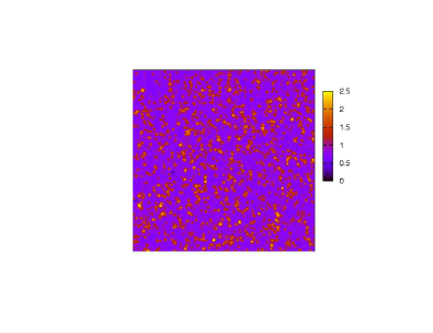
(b)

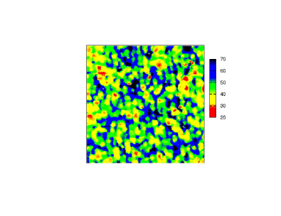
(c)

(d)

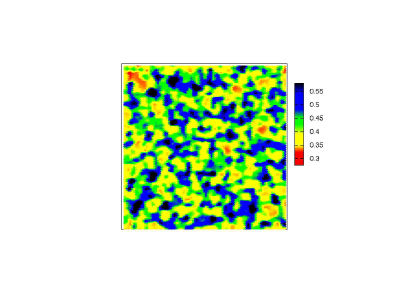
Figure 1: (Color online.) (a) Experimental $dI/dV$ map [arb. units] at -960 meV of an optimally doped BSCCO sample from Ref. DavisScience05, . (b) Experimental gap map [meV] in the same region as (a). (c) The theoretical impurity potential extracted from (a) assuming distance from plane $r_{z}=0.5$ and $\lambda=0.5$. (d) The gap map resulting from using (c) as the ’pairing potential’ in the BdG equations with $\delta g=1.5t$. Both (c) and (d) are shown in units of $t$.

Results. Fig. 1 shows, in a field of view (FOV) of $49\mbox{nm}\times 49\mbox{nm}$, the experimental LDOS at -960 meV (a), and the corresponding gap map (b) obtained by McElroy et al.DavisScience05 . The bright resonances in 1(a) reveal the location of the oxygen dopants. In Fig. 1(c) we show the impurity potential generated by using each of these dopants (833 in the above FOV) as a defect located out of the CuO₂ plane. This map resembles (a) as it should. The experimental FOV is modeled as a $90\times 90$ lattice system rotated 45 degrees with respect to the 3.83 Å  long Cu-Cu bonds, i.e. it includes $2\times 90\times 90$ sites and is aligned with the experimental FOVcomment1 . The theoretical gap map (as extracted from the LDOS) using (c) as a $\tau_{1}$ potential with $\delta g=1.5t$ at $T=0$ is shown Fig. 1(d). We find that gap maps consistent with experiment are found for $1.0<\delta g/t<2.0$. The correlation coefficient between the gap maps 1(b) and 1(d) is 0.17comment3 , a reasonably large value given the simplicity of the pure $\tau_{1}$ calculation and the fact that the correlation between the dopant positions and the experimental gap map is 0.3DavisScience05 .

(a)

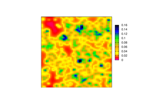
(b)

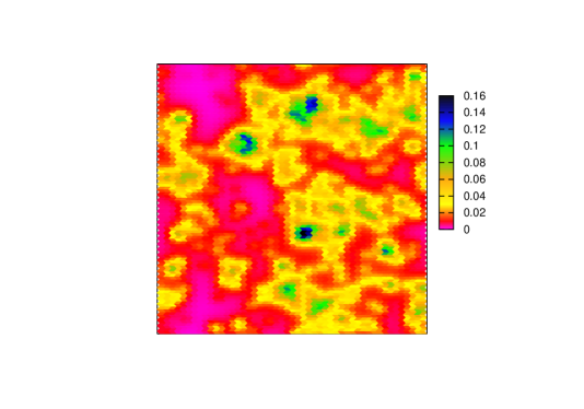
(c)

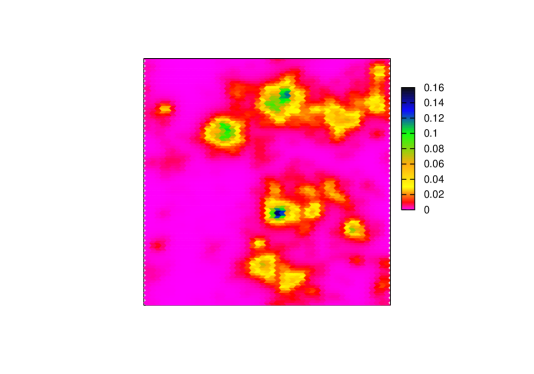
(d)

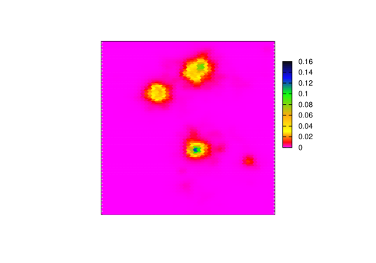
Figure 2: (Color online) OP maps, parameters from Fig. 1(d): $T\!=\!0.18t$ (a), $T\!=\!0.20t$ (b), $T\!=\!0.22t$ (c), and $T\!=\!0.24t$ (d).

Now we turn to the discussion of the results for $T\neq 0$. Below, we set $N=50$ (corresponding to the upper left 5/9th square of each image in Fig.1) and study the resulting order parameter (OP) maps, entropy $S(T)$, and specific heat $C(T)$ with focus on the temperature region near $T_{c}$. The number of iterations necessary for converged results increases dramatically near $T_{c}$, whereas just a few degrees away from $T_{c}$ we typically find that 25-50 iterations suffice. In Fig. 2, we show the OP map $\Delta_{i}=\left(\Delta_{i,i+\hat{x}}+\Delta_{i,i-\hat{x}}-\Delta_{i,i+\hat{y}}-\Delta_{i,i-\hat{y}}\right)/4,$ for temperatures near $T_{c}$. The bulk transition temperature for the homogeneous system is $T_{c0}=0.182t$. Here, one clearly sees how separate islands of finite $\Delta_{i}$ start forming above $T_{c0}$ when cooling down and eventually overlap at lower $T$. In principle, STS measurements at $T$ close to $T_{c}$ should be able to probe these superconducting islands.

In order to address the effect of the inhomogeneity on the transition widths, we first calculate the quasiparticle entropy $S(T)$ according to the well-known expression

$$S\!=\!-2\!\sum_{E_{n}>0}\!\left[f(E_{n})\ln f(E_{n})\!+\!f(-E_{n})\ln(f(-E_{n}))\right],$$ (3)

where $f(E)$ is the Fermi distribution function. From the resulting entropy $S(T)$ curve we extract the specific heat at constant volume $C(T)$ by the usual expression $C(T)=T(\partial S/\partial T)$. Fig. 3(a) compares the electronic specific heat for the clean and pair disordered systems described by different disorder strengths $\delta g$. In Fig. 3(b) we compare $C(T)$ for the different Nambu channels $\tau_{1}$ and $\tau_{3}$.

Figure 3: (Color online) Specific heat $C(T)$ for the impurity distribution of Fig. 1(c) vs $T$: (a) clean $50\times 50$ BdG system (solid, black line), ”infinite” clean system (dashed, black line), and $\tau_{1}$ disordered with $\delta g=1.0t$ (thick solid, blue line); $\delta g=1.5t$ (thick dashed, red line); $\delta g=2.0t$ (thick dash-dotted, black line). (b) Comparison of $C(T)$ for the Nambu channels $\tau_{1}$ and $\tau_{3}$ with otherwise identical impurity parameters.

We can check the BdG results by comparing to the pure ”infinite” system result (black, dashed line in Fig. 3(a)) obtained by replacing $E_{n}\rightarrow E_{\bf k}\equiv\sqrt{\epsilon_{{\bf k}}^{2}+\Delta_{{\bf k}}^{2}}$, with $\epsilon_{{\bf k}}$ the normal state dispersion with hopping integrals and chemical potential identical to the values given above, and $\Delta_{{\bf k}}=\Delta_{0}(T)(\cos k_{x}-\cos k_{y})/2$ with $\Delta_{0}(T)$ solved selfconsistently from the usual gap equation. It is clear that the $50\times 50$ BdG lattice problem is large enough to capture the sharp transition width of the clean system.

Conventional potential disorder corresponding to $\sim 10\%$ dopant atoms causes only negligible broadening in the specific heat transition width compared to the pair disordered case. This is shown in Fig. 3(b), where both curves are produced from the impurity distribution in Fig. 1(c). The transition is sharp because potential scatterers cause local suppressions of the order parameter, whereas in interstitial regions $\Delta$ decreases with temperature in a manner similar to the pure system. We have also studied distributions of strong scatterers at the percent level, and find similarly sharp transitions. On the other hand, potential disorder smooth on a scale of $\xi_{0}$ can lead to large modulations of $\mu$ which, even within BCS theory, will give larger transition widths. In this case, however, the associated local spectra are not consistent with STS measurements, as shown in Ref. NAMH05, .

As evident from 3(a), pairing disorder with parameters fixed to yield reasonable variations of the gap size and graininess at low temperatureNAMH05 leads to a broadened transition width similar to the experimental observationsLoram .

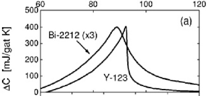
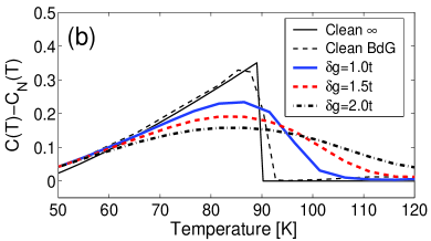
Figure 4: (Color online) (a) Specific heat transitions vs $T$ for YBCO and BSCCO optimally doped powders, from Ref. Loram, . (b) $C(T)-C_{N}(T)$ ($N$: normal state) vs $T$ with parameters from Fig.3(a), assuming that $T_{c0}=0.182t$ equals $T_{c}=90$K.

This is shown more clearly in Fig. 4, where we compare the experimental specific heat $C(T)$ for clean YBCO and optimally doped BSCCO near $T_{c}$Loram with our results for the clean and pair disordered case. It is clear that in the case of YBCO, the transition is extremely narrow, and the deviations from the mean-field treatment discussed here are consistent with weak 3DXY critical fluctuations over a range of a few degreessalamon3DXY ; hardy3DXY . On the other hand, in the case of BSCCO, it has been clear for some time that the 3DXY description of the specific heat transition is not appropriate, despite the fact that according to a naive application of the Ginzburg criterion 3DXY fluctuations should be more visiblejunod99 , and it has in fact been discussed as closer to a Bose-Einstein condensate (BEC) with specific heat exponent of $\alpha=-1$, although measured values are closer to $\alpha=-0.7$junod99 . This interpretation remains controversial, however. Other authors have suggested that a 3DXY divergence in $C(T)$ cut off by bulk nanoscale inhomogeneities over a small range $\Delta T_{c}/T_{c}\sim 0.03$ could be consistent with the dataSchneider ; Loram . Here we have put forward a similar scenario, but our microscopic model implies that the inhomogeneities dominate over a larger range $\Delta T_{c}/T_{c}\sim 0.1-0.2$ to be consistent with STS. Additional contributions from critical fluctuations must be added to the mean field effects discussed here to obtain a complete description.

Conclusions. We have presented theoretical calculations for $d$-wave superconductors with atomic scale pair disorder, using impurity parameters appropriate to reproduce semi-quantitatively the gap maps produced by STM experiments on optimally doped BSCCO, and shown that the experimental specific heat transition in this system can be explained by this model as well. This suggests that substantial nanoscale electronic inhomogeneity is characteristic of the bulk BSCCO system.

We acknowledge valuable discussions with J. C. Davis, M. Gabay, N. Goldenfeld, J. Loram, and Z. Tešanović, and thank J. C. Davis and K. McElroy for sharing their data. Partial support for this research (B. M. A. and P. J. H.) was provided by ONR N00014-04-0060. T. S. N. was supported by the A. v. Humboldt Foundation.

References

- (1) T. Cren et al., Phys. Rev. Lett. 84, 147 (2000).
- (2) S.-H. Pan et al., Nature 413, 282 (2001).
- (3) C. Howald, P. Fournier, and A. Kapitulnik, Phys. Rev. B 64, 100504(R) (2001).
- (4) K. M. Lang et al., Nature 415, 412 (2002).
- (5) S. A. Kivelson et al., Rev. Mod. Phys. 75, 1201 (2003).
- (6) J. Bobroff et al., Phys. Rev. Lett. 89, 157002 (2002).
- (7) J. W. Loram, J. L. Tallon, and W. Y. Liang, Phys. Rev. B 69, 060502R (2004).
- (8) A. Junod, A. Erb, and C. Renner, Physica C 317-318, 333 (1999).
- (9) J. W. Loram et al., Physica C 341-348, 831 (2000).
- (10) K. McElroy et al., Science 309, 1048 (2005).
- (11) T. S. Nunner et al., Phys. Rev. Lett. 95, 177003 (2005).
- (12) T. S. Nunner et al., Phys. Rev. B 73, 104511 (2006).
- (13) see, e.g. A. V. Balatsky, I. Vekhter, and J.-X. Zhu, cond-mat/0411318.
- (14) P. W. Anderson, Phys. Rev. Lett. 3, 328 (1959).
- (15) A. Ghosal, M. Randeria, and N. Trivedi, Phys. Rev. B 65, 014501 (2001).
- (16) M. Franz et al., Phys. Rev. B 56, 7882 (1997).
- (17) W. A. Atkinson, P. J. Hirschfeld, and A. H. MacDonald, Phys. Rev. Lett. 85, 3922 (2000).
- (18) A. Ghosal, M. Randeria, and N. Trivedi, Phys. Rev. B 63, 020505 (2000).
- (19) W. A. Atkinson, P. J. Hirschfeld, and L. Zhu, Phys. Rev. B 68, 054501 (2003).
- (20) A. A. Abrikosov and L. P. Gor’kov, Zh. Eksp. Teor. Fiz. 39, 1781 (1960) [Sov. Phys. JETP 12, 1243 (1961)].
- (21) M. R. Norman et al., Phys. Rev. B 52, 615 (1994).
- (22) I. Martin, D. Podolsky, and S. A. Kivelson, Phys. Rev. B 72, 060502 (2005).
- (23) K. Aryanpour et al., Phys. Rev. B 73, 104518 (2006).
- (24) A small mismatch is introduced here because the experimental FOV is slightly skewed, and will be close to, but not exactly equal to, a system.
- (25) See Ref. DavisScience05 for a definition of the correlation function.
- (26) This value of the correlation is sensitive to the details of the impurity potential: for instance, if one uses the raw LDOS data in Fig 1(a) as input, it increases to 0.3.
- (27) G. Mozurkewich, M. B. Salamon, and S. E. Inderhees, Phys. Rev. B46, 11914 (1992); A. Junod et al., Physica C 211, 304 (1993).
- (28) S. Kamal et al., Phys. Rev. Lett. 73, 1845 (1994).
- (29) T. Schneider, cond-mat/0302024.