Diffusion of a granular pulse in a rotating drum

Abstract

The diffusion of a pulse of small grains in an horizontal rotating drum is studied through discrete elements methods simulations. We present a theoretical analysis of the diffusion process in a one-dimensional confined space in order to elucidate the effect of the confining end-plate of the drum. We then show that the diffusion is neither subdiffusive nor superdiffusive but normal. This is demonstrated by rescaling the concentration profiles obtained at various stages and by studying the time evolution of the mean squared deviation. Finally we study the self-diffusion of both large and small grains and we show that it is normal and that the diffusion coefficient is independent of the grain size.

I Introduction

One of the most surprising features of mixtures of grains of different size, shape or material is their tendency to segregate (i.e., to unmix) under a wide variety of conditions Makse et al. (1998); J.B.Knight et al. (1993); Duran (2000); Ristow (2000). Axial segregation has been extensively studied experimentally Oyama (1939); Hill and Kakalios (1995); Hill et al. (1997a); Choo et al. (1997, 1998); Ristow and Nakagawa (1999); Shinbrot and Muzzio (2000); S.J.Fiedor and Ottino (2003); Newey et al. (2004); Khan et al. (2004); Losert et al. (2005); Taberlet et al. (2005a); Khan and Morris (2005a), numerically Shoichi (1998); Rapaport (2002); Taberlet et al. (2004); Taberlet et al. (2005b) and theoretically Savage (1993); Zik et al. (1994); Levitan (1997); Levine (1999); Aranson et al. (1999); Elperin and Vikhansky (1999). Yet, full understanding is still lacking. Axial segregation occurs in an horizontal rotating drum partially filled with an inhomogeneous mixture of grains. This phenomenon (also known as banding) is known to perturb industrial processes such as pebble grinding or powder mixing. After typically a hundred rotations of the drum the grains of a kind gather in well-defined regions along the axis of the drum, forming a regular pattern. When the medium consists of a binary mixture of two species of grains differing by their size, bands of small and large particles alternate along the axis of the drum. The bands of small grains can be connected through a radial core which runs throughout the whole drum Cantelaube and bideau (1995); Hill et al. (1997b). The formation of the radial core occurs quickly in the first few rotations as the small grains migrate under the surface.

Unlike radial segregation, axial segregation requires a transport of grains along the axis of the drum. Since the grains are initially mixed, they must travel along the axis of the drum to form bands. This underlines the importance of the transport mechanisms in a rotating drum. Much theoretical work as been devoted to axial segregation, most of which assumes a normal diffusion of the grains along the axis Savage (1993); Zik et al. (1994); Levitan (1997); Levine (1999); Aranson et al. (1999); Elperin and Vikhansky (1999). This hypothesis has recently been challenged by Khan et al. Khan and Morris (2005a) who have reported remarkable experimental results. These authors studied the diffusion of an initial pulse of small grains among larger grains in a long drum. Since direct visualisation is not possible (because the small grains are buried under the surface), these authors used a projection technique. Using translucent large grains and opaque small grains, they recorded the shadow obtained when a light source is placed behind the drum. They found the diffusion process to be subdiffusive and to scale approximatively as $t^{1/3}$. They also studied the self-diffusion of salt grains and found again a sub-diffusive process with an similar $t^{1/3}$ power law. In this article, we report numerical findings on the diffusion of a pulse of small grains. Interestingly, our results are in contradiction with those of Khan et al. Khan and Morris (2005a) since we observed normal diffusion.

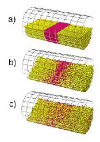
Figure 1: (Color online) Snapshots of the DEM simulation taken after 0 rotations (a), 30 rotations (b) and 100 rotations (c). A initial pulse of small (red oneline) grains is inserted a the center of a rotating drum otherwise partially filled with large grains (yellow oneline). For clarity we used here an initial pulse of length $l=25d_{S}$ in a drum of length $L=120d_{S}$. Note that longer drums are used later.

The outline of the paper is as follow. First we will describe the simulation method. A theoretical analysis of one-dimensional diffusion in a confined space is then presented. We present concentration profiles and mean squared deviation and show that the diffusion process is neither subdiffusive or superdiffusive. An instability in the average position is described. Finally, we report results on the self-diffusion of both small and large grains.

II Description of the simulation

This article presents results based on the soft-sphere molecular dynamics (MD) method, one of the Discrete Elements Methods (DEM). This method deals with deformable frictional spheres colliding with one another. Although not flawless, it has been widely used in the past two decades and has proven to be very reliable Schafer et al. (1996); Taberlet et al. (2004). Here we study the diffusion of a pulse of small grains among larger grains in an horizontal rotating drum (see Fig. 1). We follow the positions of individual small grains and in the following, it is understood that we constantly refer to the small grains. In particular, the “concentration” means concentration of small grains.

II.1 Parameters of our simulations

The mixture consists of two species of ideally spherical grains differing by their size. The small grains have a diameter $d_{S}=5$ mm and the large grains have a diameter of $2d_{S}$. The density is the same for both kinds of beads: $\rho=0.6\,\mbox{g}/\mbox{cm}^{3}$. The length of the drum, $L$, is varied from $L=60d_{S}$ to $L=420d_{S}$ and its radius is set to $20\,d_{S}$. The rotation speed is set to $0.5\,\mbox{rot}\mbox{s}^{-1}$. The grains are initially placed in a cubic grid. The small grains are placed in the middle of the drum around $x=0$ and the large grains fill up the space between the pulse of small grains and the end plates. The number of small grains can be varied but unless otherwise mentioned is set to $N=10\,300$, which corresponds to an initial pulse of length $l=25d_{S}$. The number of large grains depends of course on the length of the drum. The simulations run for typically a few hundreds of rotations.

The rotation is started and the medium compacts to lead to an average filling fraction of 37%. Radial segregation occurs rapidly (typically after five rotations of the drum) and the initial pulse is buried under the surface. The concentration profiles can be obtained at any time step. Knowing the exact position of every grain allows one to accurately compute the average position $\langle x\rangle$ and the mean squared deviation $\langle x^{2}\rangle$. Note that periodic boundary conditions could be used in order to avoid the effect of the end plates. However, the confinement would still play a role since the position of individual grains would still be limited. Moreover it may lead to nonphysical spurious effects.

II.2 The molecular dynamics method

The forces schemes used are the dashpot-spring model for the normal force $F_{ij}^{n}$ and the regularized Coulomb solid friction law for the tangential force Frenkel and Smit (1996) $F_{ij}^{t}$: respectively, $F_{ij}^{n}=k_{ij}^{n}\delta_{ij}-\gamma_{ij}^{n}\dot{\delta}_{ij}$ and $F_{ij}^{t}=\mbox{min}(\mu F_{ij}^{n},\gamma^{t}v^{s}_{ij})$, where $\delta_{ij}$ is the virtual overlap between the two particles in contact defined by: $\delta_{ij}=R_{i}+R_{j}-r_{ij}$, where $R_{i}$ and $R_{j}$ are the radii of the particles $i$ and $j$ and $r_{ij}$ is the distance between them . The force acts whenever $\delta_{ij}$ is positive and its frictional component is oriented in the opposite direction of the sliding velocity. $k_{ij}^{n}$ is a spring constant, $\gamma_{ij}^{n}$ a viscosity coefficient producing inelasticity, $\mu$ a friction coefficient, $\gamma^{t}$ a regularization viscous parameter, and $v^{s}_{ij}$ is the sliding velocity of the contact. If $k_{ij}^{n}$ and $\gamma_{ij}^{n}$ are constant, the restitution coefficient, $e$, depends on the species of the grains colliding. In order to keep $e$ constant the values of $k_{ij}^{n}$ and $\gamma_{ij}^{n}$ are normalized using the effective radius $R_{\mbox{eff}}$ defined by $1/R_{\mbox{eff}}=1/R_{i}+1/R_{j}$: $k_{ij}^{n}=k_{0}^{n}R_{0}/R_{\mbox{eff}}$ and $\gamma_{ij}^{n}=\gamma_{0}^{n}R_{\mbox{eff}}^{2}/R_{0}^{2}$. The particle/wall collisions are treated in the same fashion as particle/particle collisions, but with one particle having infinite mass and radius. The following values are used: $R_{0}=4$ mm, $k_{0}^{n}=400\;\mbox{Nm}^{-1}$, (leading to $e\simeq 0.9$), $\gamma^{t}=6\;\mbox{kg}\mbox{s}^{-1}$ and $\mu=0.3$. The value of $e$ was varied (from 0.4 to 0.9), which seemed to have only very little influence on the diffusion process.

The equations of motion are integrated using the Verlet method with a time step $dt=1/30\,\Delta t$, where $\Delta t$ is the duration of a collision ($\Delta t\approx 10^{-3}$s). The simulations are typically run for $10^{7}$ time steps, corresponding to a few hundreds of rotations.

III 1D confined diffusion

Before analyzing any results, one should quantify the influence of the end-plates. The limited space imposes some constraints on the diffusion process: the position $x$ along the axis of the drum can only range from $-L/2$ to $L/2$ which imposes a limit to the mean squared deviation. In order to clarify the effect of the confinement we present in this section a theoretical analysis of an initial Dirac distribution (corresponding to the initial pulse) diffusing in a confined 1D space. Note that an initial pulse function could also be used. However, this would add a degree of complexity to the problem without much benefit. In this brief section we only intend to qualitatively describe the effect of the confinement rather than studying it in details. The concentration, defined for $x\in[-L/2,L/2]$, is given by Carslaw and Jaeger (1959):

$$c(x,t)=\displaystyle\frac{1}{\sqrt{4\,\pi\,D\,t}}\;\displaystyle\sum_{n=-\infty}^{\infty}\exp^{\displaystyle\frac{-(x+n\,L)^{2}}{4\,D\,t}}.$$

Note that the exact solution for an initial pulse of nonzero width can be obtained by convoluating this solution to the initial pulse function.

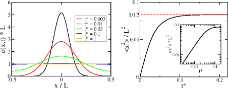
Figure 2: (Color online) Left: concentration profiles obtained at various stages for a confined 1D diffusion process. Right: mean squared deviation versus dimensionless time. At short times the function is a linear function of time but at longer time $\langle x^{2}\rangle$ saturates. Inset: the data plotted on a log-log scale.

We can now plot the concentration profiles for various times (see Fig. 2). Note that the time and position can be made dimensionless (using $t^{*}=t\,L/D^{2}$ and $x^{*}=x/L$). One can see that at short time the distribution is almost a Gaussian but at longer times, the confinement plays a important role. The distribution flattens and eventually reaches a constant value of $c(x)=1/L$, which corresponds to a mean squared deviation $\langle x^{2}\rangle_{\infty}=L^{2}/12$. Figure 2 also shows the time evolution of the mean squared deviation defined here by $\langle x^{2}\rangle=\int_{0}^{L}c(x,t)\,x^{2}\,dx$. The function is clearly linear at short time (as confirmed by the log-log scale inset) but saturates a longer times. This behavior was expected but can lead to erroneous conclusions. Indeed, the curvature observed in $\langle x^{2}\rangle(t)$ could be mistaken for a sign of a subdiffusive process whereas it is solely due to the confinement. Note that Khan et al. Khan and Morris (2005a) used a rather long tube in their experiments, meaning that the confinement did not affect their results.

IV Results

IV.1 Concentration profiles

We now present results obtained in our 3D numerical simulations. The position of every grain at any time step is known, which allows one to compute the concentration profiles. The drum is divided in virtual vertical slices of length $d_{S}$ and the number of grains whose center is in a given slice is computed. Figure 3 shows concentration profiles of small grains measured at short times for a drum of length $L=420\,d_{S}$. Note that the profiles tend toward Gaussian distributions as the grains slowly diffuse in the drum.

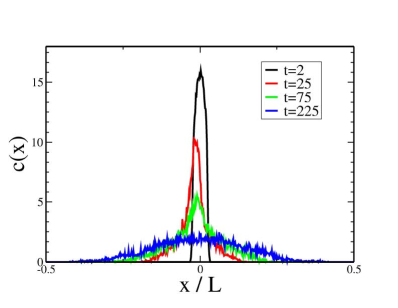
Figure 3: (Color online) Concentration profiles at different time obtained with a drum of length $L=420\,d_{S}$.

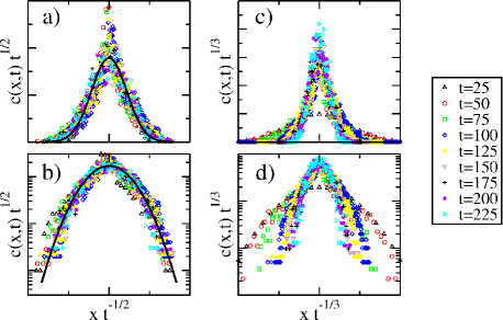
Figure 4: (Color online) Rescaled concentration profiles (in arbitrary units) at different times obtained with a drum of length $L=420\,d_{S}$. The data is rescaled using $t^{1/2}$ for (a) and (b), and $t^{1/3}$ for (c) and (d). (a) and (c): linear scale, (b) and (d): semilog scale. The solid line on (a) and (b) is a Gaussian fit at $t=225$ rotations. On can see that the $t^{1/2}$ rescaling leads to a good collapse unlike the $t^{1/3}$ rescaling. This is particularly clear on the semilog plots.

Note that no axial segregation is visible at any point. Indeed, except for the obvious one at $x=0$, there is no peak in the concentration. We believe that the number of small grains is too small compared to that of large grains to trigger axial segregation.

A very good test to check whether the diffusion process is subdiffusive, normal or superdiffusive is to try to collapse various concentration profiles at different times onto one unique curve. This should be done by dividing the position by some power of the time ($t^{\alpha}$) and for reasons of normalization (i.e. mass conservation) by simultaneously multiplying the concentration by $t^{\alpha}$. The process is subdiffusive if $\alpha<1/2$, normal if $\alpha=1/2$ and super-diffusive if $\alpha>1/2$. Using the profiles taken at “short times” (i.e., before the confinement plays a role), we were able to obtain an excellent collapse of our data using the value $\alpha=1/2$. Figures 4(a) and 4(b) shows the data in a linear and semilog scales. Figures 4(c) and 4(d) shows similar plots obtained using $\alpha=1/3$, as suggested by Khan et al. Khan and Morris (2005a). The first conclusion that can be drawn is that the collapse is excellent for $\alpha=1/2$ and poor for $\alpha=1/3$. This is particularly clear on the semilog plots. The profiles on Fig. 4(d) tend to narrow with increasing time whereas no trend is visible on Fig. 4(b). This clearly shows that in our simulations the diffusion is a normal diffusion process. Moreover, the collapsed data can be well fitted by a Gaussian distribution, as clearly evidenced by the semilog plot on Fig. 4(b).

IV.2 Mean squared deviation

The collapse of the different curves on Fig. 4 is a good indication that the diffusion process in normal. An even better test is to plot the time evolution of the mean squared deviation defined here by $\langle x^{2}\rangle=1/N\,\sum_{i}(x_{i}-x_{i}^{0})^{2}$ where $x_{i}^{0}$ is the initial position of the grain number $i$. Figure 5a is a plot of the mean squared deviation versus time obtained for various values of $L$. Of course the saturation value $\langle x^{2}\rangle_{\infty}$ is different for different values of $L$ but one can see that the initial slope is the same for all curves. This shows that the diffusion coefficient is well defined at “short times” and does not depend on the length of the drum. Figure 5(b) is a rescaled plot of the same data. The time is divided by $L^{2}$ and the mean squared deviation by $\langle x^{2}\rangle_{\infty}$. One can see that all data collapse at short times, showing again that the diffusion coefficient is well defined and that it is independent of $L$.

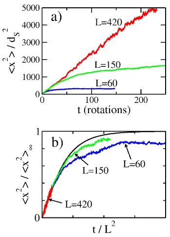
Figure 5: (Color online) (a) Mean squared deviation versus time (in arbitrary units). (b) Rescaled data. The different curves correspond to different values of the drum length: Blue oneline: $L=60\,d_{S}$, green online $L=150\,d_{S}$ red oneline : $L=420\,d_{S}$. The solid line in (b) is the theoretical prediction.

One can see on Fig. 5(b) that the mean squared deviation does not reach the theoretical saturation value $\langle x^{2}\rangle_{\infty}$. This is an indication that in the final state the concentration is not uniform. Indeed although no segregation bands are visible there is still a signature of axial segregation. The concentration profile in the steady state obtained for $L=60\,d_{S}$ is shown on Fig. 6. One can see that the initial central peak has diffused but the concentration is not even in the final state: the concentration drops near the end plate, which has also been observed experimentally. This explains why the saturation value $\langle x^{2}\rangle_{\infty}=L^{2}/12$ is not reached in our simulations. Note, however, that for longer drums this effect becomes negligible.

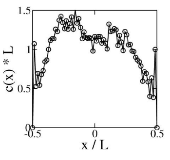
Figure 6: (Color online) Steady state concentration profile for $L=60d_{S}$ after 150 rotations. The distribution is not perfectly uniform: the concentration in small grains drops near the end plates.

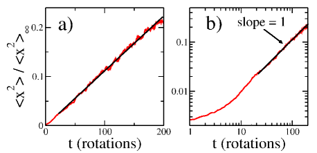
Figure 7: (Color online) Mean squared deviation versus time in a linear (right) and log-log (left) scale for $L=420d_{S}$. Except for a brief transient during which radial segregation occurs $\langle x^{2}\rangle$ is a linear function of time the data plotted in a log-log plot scale is extremely well fitted by a line of slope 1.

The rescaled plot on Fig. 5b allows one to decide which time frame should be considered “short times”. In particular it is obvious from that picture that the run performed with $L=420\,d_{S}$ has not yet been affected by the end-plates after 200 rotations. Therefore, it allows one to study the diffusion process without considering the consequences of the confinement. Figure 7 shows the mean squared deviation versus time in linear and log-log scales for a drum length $L=420\,d_{S}$. Both plots clearly demonstrate that the diffusion is normal. Indeed, the data on Fig. 7 is well-fitted by a straight line on a linear scale. Similarly, after a short transient corresponding to the time it takes for radial segregation to be completed (approximatively 10 rotations here), the data plotted in a log-log scale is perfectly fitted by a line of slope 1 for over a decade. These observations show without a doubt that the diffusion process in our simulations is neither subdiffusive nor superdiffusive but simply normal.

V Self-diffusion

In this section we will study the self-diffusion process. We would like to compare results obtained with three runs. The first run consists of monodisperse small particles, the second of large particles and the third one is the pulse experiment described above. The rotation speed, filling ratio and drum size are identical all three cases. In order to save computational time, we used a rather short drum ($L=60d_{S}$). The major difference between a self-diffusion numerical experiment and the diffusion of a pulse is that no radial segregation can exist in the self-diffusion. Since the mixture is monodisperse there cannot exist any form of segregation. It is therefore interesting to compare the two numerical experiments and elucidate the role of the radial segregation in the diffusion process.

What should be measured in a self-diffusion experiment? Of course, there is no initial pulse in the drum but one can be arbitrarily defined. Indeed, one can track the grains whose initial position were within a given distance from the center of the drum. This would allow to plot “virtual concentration profiles.” More simply, we can use the definition used before for the mean squared deviation $\langle x^{2}\rangle=1/N\,\sum_{i}(x_{i}-x_{i}^{0})^{2}$. Note, however, that the end plates play the same role as before. Indeed, the position is still limited. Moreover, the grains initially located near an end plate will “feel” the end plates at early stages. It is therefore necessary to measure the mean squared deviation of grains initially centered around $x=0$. For both self-diffusion simulations we used the grains located within a distance of $10d_{S}$ from the center of the drum ($x=0$).

Figure 8 is a plot of $\langle x^{2}\rangle$ versus time for all three runs. Rather surprisingly, all three curve collapse. This shows that the diffusion process is independent of the grain size, which is very interesting. One could expect the diffusion coefficient to scale with the grain diameter and the two self-diffusion coefficients to be different but it is obviously not the case. Instead, our simulations show that $d_{S}$ is not a relevant length scale regarding the diffusion process.

Maybe even more interestingly, the data collapse shows that radial segregation does not seem to affect the diffusion process. Indeed, the diffusivity is the same in the pulse experiment (where radial segregation exist) as in the self-diffusion experiments (where no segregation can exist).

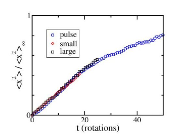
Figure 8: (Color online) Mean squared deviation versus time for the pulse experiment (blue oneline), self-diffusion of small (red oneline) and large (black) grains. One can see all three curves collapse, showing that the self-diffusion is normal and that the diffusion coefficient is independent of the grain size.

VI Discussion and conclusion

The diffusion of an initial pulse seems to be very helpful in understanding the basic mechanisms leading to axial segregation. It is however difficult to obtain precise measurements in an experimental system. Khan et al. Khan and Morris (2005a) developed a clever projection technique which allows one to observe the hidden core of small grains. The shadow projected by the opaque small grains is clearly related to the concentration in small grains but one can question whether the link between the two is a linear relation or a more complex one.

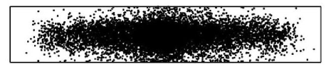
Figure 9: View of the small grains projected perpendicularly to the free surface for $L=280d_{s}$ after 75 rotations (i.e., before the confinement plays a role).

Our numerical simulations show consistent results indicating that the diffusion is normal. This conclusion is strongly supported by a collapse of concentrations profiles rescaled by $t^{1/2}$. Moreover, the mean squared deviation is clearly a linear function of time as long as the confinement does not play a role. These results are in strong contradiction with those obtained experimentally by Khan et al. Khan and Morris (2005a). These authors found a subdiffusive process which scales approximatively as $t^{1/3}$. The origin of this discrepancy remains unknown.

It could originate from the force models used in our simulations. In particular, it would be very interesting to test the consistency of our results using the Hertz modelor a tangential spring friction model Schafer et al. (1996) . The discrepancy might also originate in the projection method used by Khan et al. Khan and Morris (2005a) which is an indirect measurement of the concentration. However, it seems unlikely that the details of the projection techniuqe would change the diffusion power laws. One interesting check for that method would be to apply the projection technique to our numerical data. Figure 9 shows a projection (perpendicularly to the free surface) of the core of small grains obtained for $L=280d_{s}$ after 75 rotations. This image looks rather differents from those of Khan et al. Khan and Morris (2005a). In particular, one can observe individual grains, which is not possible using their projection technique. Applying the projection technique to our numerical data is not straightforward and the definition of such a procedure would obviously drastically influence the outcome. Note, however, that Khan et al. have also observed a subdiffusive self-diffusion using direct imaging, which does not involve projection. This supports the idea that the 1/3 power law which they reported is not an artifact of their projection technique and that the origin of the discrepancy between the experiments and the simulations may be due to some unaccounted for physical effect.

After stimulating discussions with these authors, we believe that there are a number a physical differences between our two system that might lead to different results. One difference between the two systems is the ratio of the drum diameter to the avarage particle diameter $\delta=D/\bar{d}$. In our simulations $\delta=26$ and in their experiments $\delta\approx 100$. The discrepancy might also be caused by the difference in the shape of the grains although a subdifussive process was observed experimentally using bronze beads. Finally, the experiments were conducted in a humidity-controlled room and the capillary bridges between the grains might have modified the diffusion process.

In conclusion, our numerical results showed that the diffusion along the axis of the drum is normal. Having studied the effect of the confinement, we can conclude that the curvature observed in the mean squared deviation is not a sign of subdiffusion. The rescaled concentration profiles lead to the same conclusion that the diffusion process is normal. The study of self-diffusion shows that the diffusivity is independent of the grain size and is not affected by radial segregation. This results may shed some light on the mechanisms of formation of segregation bands since it indicates that the transport of grains along the axis of the drum is identical for both species of grains. We hope that these results will inspire theoretical models and help understanding the puzzling phenomenon of axial segregation.

VII Acknowledgements

The authors would like to thank M. Newey, W. Losert, Z. Khan and S.W. Morris for fruitful discussions.

References

- Makse et al. (1998) H. A. Makse, R. C. Ball, H. E. Stanley, and S. Warr, Phys. Rev. E 58, 3357 (1998).
- J.B.Knight et al. (1993) J.B.Knight, H.M.Jaeger, and S.R.Nagel, Phys. Rev. Lett. 70, 3728 (1993).
- Duran (2000) J. Duran, Sand, Powders and Grains: An Introduction to the Physics of Granular Material (Springer, New York, 2000).
- Ristow (2000) G. Ristow, Pattern Formation in Granular Materials (Springer, New York, 2000).
- Oyama (1939) Y. Oyama, Bull. Inst. Phys. Chem. Res. Rep. 5, 600 (1939).
- Hill and Kakalios (1995) K. M. Hill and J. Kakalios, Phys. Rev. E 52, 4393 (1995).
- Hill et al. (1997a) K. M. Hill, A. Caprihan, and J. Kakalios, Phys. Rev. Lett. 78, 50 (1997a).
- Choo et al. (1997) K. Choo, M. W. Baker, T. C. A. Moltena, and S. W. Morris, Phys. Rev. Lett. 79, 2975 (1997).
- Choo et al. (1998) K. Choo, T. C. A. Moltena, and S. Morris, Phys. Rev. E 58, 6115 (1998).
- Ristow and Nakagawa (1999) G. H. Ristow and M. Nakagawa, Phys. Rev. E 59, 2044 (1999).
- Shinbrot and Muzzio (2000) T. Shinbrot and F. Muzzio, Phys. Today 53,p. 25 (2000).
- S.J.Fiedor and Ottino (2003) S.J.Fiedor and J. Ottino, Phys. Rev. Lett. 91, 244301 (2003).
- Newey et al. (2004) M. Newey, J. Ozik, S. V. der Meer, E. Ott, and W. Losert, Europhys. Lett. 66, 205 (2004).
- Khan et al. (2004) Z. S. Khan, W. Tokaruk, and S. Morris, Europhys. Lett. 66, 212 (2004).
- Losert et al. (2005) W. Losert, M. Newey, N. Taberlet, and P. Richard, in Powders & Grains 2005, edited by Garcia-Rojo, Hermann, and McNamara (Balkema, Rotterdam, 2005), p. 845.
- Taberlet et al. (2005a) N. Taberlet, P. Richard, M. Newey, and W. Losert, in Powders & Grains 2005, edited by R. Garcia-Rojo, H.J. Herrmann, and S. McNamara (Balkema, Rotterdam, 2005a), p. 853.
- Khan and Morris (2005a) Z. S. Khan and S. W. Morris, Phys. Rev. Lett. 94, 048002 (2005a).
- Shoichi (1998) S. Shoichi, Mod. Phys. Lett. B 12, 115 (1998).
- Rapaport (2002) D. C. Rapaport, Phys. Rev. E 65, 061306 (2002).
- Taberlet et al. (2004) N. Taberlet, W. Losert, and P. Richard, Europhys. Lett. 68, 522 (2004).
- Taberlet et al. (2005b) N. Taberlet, M. Newey, P. Richard, and W. Losert, unpublished (2005b).
- Savage (1993) S. Savage, in Disorder and Granular Media, edited by D. Bideau and A. Hansen (North-Holland, Amsterdam, 1993), p. 255.
- Zik et al. (1994) O. Zik, D. Levine, S. G. Lipson, S. Shtrikman, and J. Stavans, Phys. Rev. Lett. 73, 644 (1994).
- Levitan (1997) B. Levitan, Phys. Rev. E 58, 2061 (1997).
- Levine (1999) D. Levine, Chaos 9, 573 (1999).
- Aranson et al. (1999) I. S. Aranson, and L. S. Tsimring, Phys. Rev. Lett. 82, 4643 (1999).
- Elperin and Vikhansky (1999) T. Elperin and A. Vikhansky, Phys. Rev. E 60, 1946 (1999).
- Cantelaube and bideau (1995) F. Cantelaube and D. Bideau, Europhys. Lett. 30, 133 (1995).
- Hill et al. (1997b) K. M. Hill, A. Caprihan, and J. Kakalios, Phys. Rev. E 56, 4386 (1997b).
- Schafer et al. (1996) J. Schäfer, S. Dippel, and D. Wolf, J. Phys. I 6, 5 (1996).
- Frenkel and Smit (1996) D. Frenkel and B. Smit, Understanding Molecular Simulations. From Algorithms to Applications (Academic Press, San Diego, California, 1996).
- Carslaw and Jaeger (1959) H. Carslaw and J. Jaeger, Conduction of Heat in Solids (Oxford University Press, Oxford, U.-K., 1959).