A Fiber Bundle Model of Traffic Jams

Abstract

We apply the equal load-sharing fiber bundle model of fracture failure in composite materials to model the traffic failure in a system of parallel road network in a city. For some special distributions of traffic handling capacities (thresholds) of the roads, the critical behavior of the jamming transition can be studied analytically. This has been compared with that for the asymmetric simple exclusion process in a single channel or road.

1 Introduction

Traffic jams or congestions occur essentially due to the excluded volume effects (among the vehicles) in a single road and due to the cooperative (traffic) load sharing by the (free) lanes or roads in multiply connected road networks (see e.g., [1]). We will discuss here briefly how the Fiber Bundle Model (FBM) for fracture failure in composite materials (see e.g, [2]) can be easily adopted for the study of (global) traffic jam in a city network of roads. In the equal-load-sharing FBM, the load carried by the failed fibers is transferred and shared uniformly by the other surviving fibers in the bundle and therefore the dynamics of failure propagation in the system is analytically tractable [2]. Using this model for the traffic network, it is shown here that the generic equation for the approach of the jamming transition in FBM corresponds to that for the Asymmetric Simple Exclusion Processes (ASEP) leading to the transport failure transition in a single channel or lane (see e.g., [3]).

2 Model

Let the suburban highway traffic, while entering the city, get fragmented equally through the various narrower streets within the city and get combined again outside the city (see Fig. 1). Let the input traffic current be denoted by $I_{O}$ and the total output traffic current be denoted by $I_{T}$. In the steady state, without any global traffic jam, $I_{T}=I_{O}$. In case, $I_{T}$ falls below $I_{O}$, the global jam starts and soon $I_{T}$ drops to zero. This occurs if $I_{O}>I_{c}$, the traffic current in the network beyond which global traffic jam occurs. The steady state flow picture then looks as shown in Fig. 2. Let us assume that the parallel roads within the city have got different thresholds for traffic handling capacity: $i_{c_{1}},i_{c_{2}},\ldots,i_{c_{N}}$ for the $N$ different roads (the $n$-th road gets jammed if the traffic current $i$ per road exceeds $i_{c_{n}}$). Initially $i=I_{O}/N$ and increases as some of the roads get jammed and the same traffic load $I_{i}$ has to be shared equally by a lower number of unjammed roads. Next, we assume that the distribution $\rho(i_{c})$ of these thresholds is uniform (see Fig. 3) upto a maximum threshold current (corresponding to the widest road traffic current capacity), which is normalized to unity (sets the scale for $I_{c}$).

Figure 1: The highway traffic current $I_{O}$ gets fragmented into $i^{\prime}s$ and the narrower roads having threshold current $i_{c_{n}}\leq i$ gets congested or blocked and this extra traffic load per uncongested roads get equally distributed, causing further blocking of some more roads.

The jamming dynamics in this model starts from the $n$-th road (say in the morning) when the traffic load $i$ per city roads exceeds the threshold $i_{c_{n}}$ of that road. Due to this jam, total number of intact or uncongested roads decreases and rest of these roads have to bear the entire traffic load in the system. Hence effective traffic load or stress on the uncongested roads increases and this compels some more roads to fail or get jammed. These two sequential operations, namely the stress or traffic load redistribution and further failure in service of roads continue till an equilibrium is reached, where either the surviving roads are strong (wide) enough to share equally and carry the entire traffic load on the system (for $I_{O}<I_{c}$) or all the roads fail (for $I_{O}\geq I_{c}$) and a (global) traffic jam occurs in the entire) road network system (to be brought back perhaps in the night when the load $I_{O}$ decreases much below $I_{c}$).

3 Jamming dynamics

This jamming dynamics can be represented by recursion relations in discrete time steps. Let us define $U_{t}(i)$ to be the fraction of uncontested roads in the network that survive after (discrete) time step $t$, counted from the time $t=0$ when the load (at the level $I_{O}=iN$) is put in the system (time step indicates the number of stress redistributions). As such, $U_{t}(i=0)=1$ for all $t$ and $U_{t}(i)=1$ for $t=0$ for any $i$; $U_{t}(i)=U^{*}(i)\neq 0$ for $t\to\infty$ if $I_{O}<I_{c}$, and $U_{t}(i)=0$ for $t\to\infty$ if $I_{O}>I_{c}$.

Figure 2: Traffic jam (global) in the network of roads occurs when $I_{O}~{}>~{}I_{c}$, the threshold traffic capacity of the city road-network.

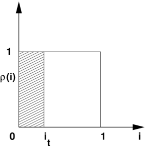
Figure 3: The simple model considered here assumes uniform density $\rho(i)$ of the road traffic flow capacity distribution up to a cutoff capacity (normalized to unity). At any traffic load per road level $i_{t}$ at time $t$, the fraction $i_{t}$ of roads fails and fraction $1-i_{t}$ survives.

Therefore $U_{t}(i)$ follows a simple recursion relation (see Fig. 3)

$$U_{t+1}=1-i_{t};\ \ i_{t}=\frac{I_{O}}{U_{t}N}$$

$${\rm or,}\ \ U_{t+1}=1-\frac{i}{U_{t}}.$$ (1)

In equilibrium $U_{t+1}=U_{t}=U^{*}$ and thus (1) is quadratic in $U^{*}$ :

$$U^{*^{2}}-U^{*}+i=0.$$

The solution is

$$U^{*}(i)=\frac{1}{2}\pm(i_{c}-i)^{1/2};i_{c}=\frac{1}{4}.$$

Here $i_{c}=I_{c}/N$ is the critical value of traffic current (per road) beyond which the bundle fails completely. The quantity $U^{*}(i)$ must be real valued as it has a physical meaning: it is the fraction of the roads that remains in service under a fixed traffic load $i$ when the traffic load per road lies in the range $0\leq i\leq i_{c}$. Clearly, $U^{*}(0)=1$. The solution with ($+$) sign is therefore the only physical one. Hence, the physical solution can be written as

$$U^{*}(i)=U^{*}(i_{c})+(i_{c}-i)^{1/2};\ U^{*}(i_{c})=\frac{1}{2}\ {\rm and}\ i_{c}=\frac{1}{4}.$$ (2)

For $i>i_{c}$ we can not get a real-valued fixed point as the dynamics never stops until $U_{t}=0$ when the network gets completely jammed.

4 Critical behavior

(a) At $i<i_{c}$

It may be noted that the quantity $U^{*}(i)-U^{*}(i_{c})$ behaves like an order parameter that determines a transition from a state of partial failure of the system($i\leq i_{c}$) to a state of total failure ($i>i_{c}$) :

$$O\equiv U^{*}(i)-U^{*}(i_{c})=(i_{c}-i)^{\beta};\beta=\frac{1}{2}.$$ (3)

To study the dynamics away from criticality ($i\rightarrow i_{c}$ from below), we replace the recursion relation (1) by a differential equation

$$-\frac{dU}{dt}=\frac{U^{2}-U+i}{U}.$$

Close to the fixed point we write $U_{t}(i)=U^{*}(i)$ + $\epsilon$ (where $\epsilon\rightarrow 0$). This gives

$$\epsilon=U_{t}(i)-U^{*}(i)\approx\exp(-t/\tau),$$ (4)

where $\tau=\frac{1}{2}\left[\frac{1}{2}(i_{c}-i)^{-1/2}+1\right]$. Thus, near the critical point (for jamming transition) we can write

$$\tau\propto(i_{c}-i)^{-\alpha};\alpha=\frac{1}{2}.$$ (5)

Therefore the relaxation time diverges following a power-law as $i\rightarrow i_{c}$ from below.

One can also consider the breakdown susceptibility $\chi$, defined as the change of $U^{*}(i)$ due to an infinitesimal increment of the traffic stress $i$

$$\chi=\left|\frac{dU^{*}(i)}{di}\right|=\frac{1}{2}(i_{c}-i)^{-\gamma};\gamma=\frac{1}{2}.$$ (6)

Hence the susceptibility diverges as the applied stress $i$ approaches the critical value $i_{c}=\frac{1}{4}$. Such a divergence in $\chi$ can be clearly observed in the numerical study of these dynamics.

(b) At $i=i_{c}$

At the critical point ($i=i_{c}$), we observe a different dynamic critical behavior in the relaxation of the failure process. From the recursion relation (1), it can be shown that decay of the fraction $U_{t}(i_{c})$ of uncongested roads that remain in service at time $t$ follows a simple power-law decay :

$$U_{t}=\frac{1}{2}(1+\frac{1}{t+1}),$$ (7)

starting from $U_{0}=1$. For large $t$ ($t\rightarrow\infty$), this reduces to $U_{t}-1/2\propto t^{-\delta}$; $\delta=1$; a power law, and is a robust characterization of the critical state.

5 Universality class of the model

The universality class of the model can be checked (cf. [2]) taking two other types of road capacity distributions $\rho(i)$: (I) linearly increasing density distribution and (II) linearly decreasing density distribution of the current thresholds within the limit $0$ and $1$. One can show that while $i_{c}$ changes with different strength distributions ($i_{c}=\sqrt{4/27}$ for case (I) and $i_{c}=4/27$ for case II), the critical behavior remains unchanged: $\alpha=1/2=\beta=\gamma$, $\delta=1$ for all these equal (traffic) load sharing models.

6 Transport in ASEP

Figure 4: The transport current $I$ in the one dimensional lane or road is possible if, say, the $i$-th site is occupied and the $(i+1)$-th site is vacant. The inter-site hopping probability is indicated by $J$.

Let us consider the simplest version of the asymmetric simple exclusion process transport in a chain (see Fig. 4). Here transport corresponds to movement of vehicles, which is possible only when a vehicle at site $i$, say, moves to the vacant site $i+1$. The transport current $I$ is then given by (see e.g., [3])

$$I=J\rho_{i}(1-\rho_{i+1}),$$ (8)

where $\rho_{i}$ denotes the site occupation density at site $i$ and $J$ denotes the inter-site hopping probability. The above equation can be easily recast in the form

$$\rho_{i+1}=1-{\frac{\sigma}{\rho_{i}}},$$ (9)

where $\sigma=I/J$. Formally it is the same as the recursion relation (1) for the density of uncongested roads in the FBM model discussed above; the site index here in ASEP plays the role of time index in FBM.

7 Summary and discussion

We have applied here the equal load-sharing fiber bundle model of fracture failure in composite materials to model the traffic failure in a network of parallel roads in a city. For some special distributions of traffic handling capacities (thresholds) of the roads, namely uniform and also linearly increasing or decreasing density of road capacities, the critical behavior of the jamming transition has been studied analytically. This dynamics of traffic jam progression (given by the recursion relation (1), for uniform density of road capacity, as shown in Fig. 3 ) has been compared with that for the asymmetric simple exclusion process (9) in a single channel or road; the exact correspondence indicates identical critical behavior in both the cases. The same universality for other cases of $\rho(i)$ in FBM suggests similar behavior for other equivalent ASEP cases as well.

References

- [1] D. Chowdhury, L. Santen and A. Schadschnider, Phys. Rep. 329 199 (2000)
- [2] S. Pradhan and B. K. Chakrabarti, Int. J. Mod. Phys. B 17 5565 (2003)
- [3] R. B. Stinchcombe, Adv. Phys. 50 431 (2001).