The fate of orbitons coupled to phonons

Abstract

The key feature of an orbital wave or orbiton is a significant dispersion, which arises from exchange interactions between orbitals on distinct sites. We study the effect of a coupling between orbitons and phonons in one dimension using continuous unitary transformations (CUTs). Already for intermediate values of the coupling, the orbiton band width is strongly reduced and the spectral density is dominated by an orbiton-phonon continuum. However, we find sharp features within the continuum and an orbiton-phonon anti-bound state above. Both show a significant dispersion and should be observable experimentally.

I Introduction

In correlated electron systems, orbital degeneracy is discussed as an interesting source for very rich physics Tokura and Nagaosa (2000); Khomskii (2005); Khaliullin (2005). The orbital degeneracy may be lifted by a coupling to phonons Jahn and Teller (1937) and/or by superexchange processes Kugel and Khomskii (1973). The latter give rise to an intimate connection between spin and orbital degrees of freedom. Spin-orbital models predict interesting ground states such as orbital order or quantum-disordered orbital-liquid states, and one may expect novel elementary excitations: dispersive low-energy orbital waves termed orbitons Ishihara et al. (2005). Experimentally, the observation of orbitons has been claimed on the basis of Raman data of the orbitally ordered compounds LaMnO₃ Saitoh et al. (2001) and RVO₃ (R=La, Nd, Y) Miyasaka et al. (2005); Sugai and Hirota (2006). In LaMnO₃, the bosonic orbitons are treated similar to magnons in a long-range spin-ordered state, whereas the orbital excitations of RVO₃ are discussed in terms of one-dimensional (1D) fermions equivalent to the spinons of a 1D Heisenberg chain Saitoh et al. (2001); Miyasaka et al. (2005); Ishihara et al. (2005).

The role attributed to phonons varies largely. For the case of LaMnO₃, it has been argued that the orbiton-phonon coupling constant $g$ is small, only giving rise to a small shift of the orbiton band Saitoh et al. (2001); Ishihara et al. (2005). The dynamical screening of orbitons by phonons and the mixed orbiton-phonon character of the true eigen modes has been studied by van den Brink van den Brink (2001) using self-consistent second order perturbation theory (SOPT) in the orbiton-phonon coupling $g$. He interpreted the Raman peaks observed at about 160 meV in LaMnO₃ Saitoh et al. (2001) in terms of phonon satellites of the orbiton band, assuming weak coupling $g$. In contrast, Allen and Perebeinos Allen and Perebeinos (1999) argued that the coupling $g$ is so strong that the eigen modes can be described in terms of local crystal-field excitations (‘vibrons’). Then, the spectral density consists of a series of phonon sidebands (Franck-Condon effect) with a center frequency $>1$ eV Allen and Perebeinos (1999). Experimentally, the orbiton interpretation of the Raman features observed at about 160 meV in LaMnO₃ has been strongly questioned based on the comparison with infrared data Grüninger et al. (2002); Rückamp et al. (2005), which clearly indicate that these features should be interpreted in terms of multiphonons.

The ‘non-local’ collective character of the orbital excitations is relevant if the energy scale of the superexchange is larger than the coupling to the phonons. At present, a systematically controlled quantitative description of the gradual transition from well-defined dispersive orbitons at $g$=0 to predominantly ‘local’ crystal-field excitations for strong coupling is still lacking. The SOPT treatment is valid at small $g$. Qualitatively, it shows (i) a polaronic reduction of the orbiton band width van den Brink (2001) due to the dressing of the orbiton by a phonon cloud yielding a heavy quasi-particle, and (ii) a transfer of spectral weight from the orbiton band to phonon side-bands, i.e., to a broad and featureless orbiton-phonon continuum (see below). This suggests that signatures of collective behavior are rapidly washed out with increasing $g$.

We perform a well-controlled calculation of the spectral line shape of the orbitons at larger values of $g$ which elucidates the collective character of the excitations. Our study is based on continuous unitary transformations (CUTs) Głazek and Wilson (1993); Wegner (1994); Knetter and Uhrig (2000) realized in a self-similar manner Mielke (1997) in real space Reischl et al. (2004). For clarity and simplicity, we restrict ourselves to the minimal model in one spatial dimension (1D). We find that well-defined, dispersive features appear in the orbiton-plus-one-phonon continuum for intermediate values of $g$. Additionally, a sharp orbiton-phonon anti-bound state (ABS) is formed above the continuum. Both phenomena should allow to observe dispersive signatures of orbitons in experiment.

II Model

We study the following Hamiltonian in one dimension

$$H_{0} = \sum_{i}\left(\omega_{\rm orb}^{\rm ex}+\omega_{\rm orb}^{\rm JT}\right)c^{\dagger}_{i}c^{\phantom{\dagger}}_{i}-\frac{J}{4}\sum_{i}\left(c^{\dagger}_{i+1}c^{\phantom{\dagger}}_{i}+c^{\dagger}_{i-1}c^{\phantom{\dagger}}_{i}\right)$$ (1)

$$+ \omega_{\rm ph}\sum_{i}b^{\dagger}_{i}b^{\phantom{\dagger}}_{i}+2g\sum_{i}c^{\dagger}_{i}c^{\phantom{\dagger}}_{i}\left(b^{\dagger}_{i}+b^{\phantom{\dagger}}_{i}\right)$$

where $c$ and $b$ are bosonic operators that represent orbitons and phonons, respectively, $\omega_{\rm orb}^{\rm ex}$ and $\omega_{\rm orb}^{\rm JT}=4g^{2}/\omega_{\rm ph}$ denote the contributions to the local orbiton energy from superexchange and from a static Jahn-Teller deformation van den Brink (2001), $J$ the superexchange coupling constant, $\omega_{\rm ph}$ the phonon energy, and $g$ the coupling between orbitons and phonons. The Jahn-Teller energy $\omega_{\rm orb}^{\rm JT}=4g^{2}/\omega_{\rm ph}$ results from the static distortion of the local environment of the transition-metal ion with orbital degeneracy. This distortion lifts the degeneracy such that the orbitals are split into a low-lying orbital termed ground state orbital and a higher-lying one. The orbital excitation consists in lifting an electron from the ground state orbital into the higher-lying one. This is the effect of the creation operator $c^{\dagger}$. The superexchange $J$ acts as a hopping amplitude of the orbiton, giving rise to a dispersion.

The Hamiltonian (1) is the bosonic version of the well-investigated 1D Holstein model of coupled electrons and phonons yielding polarons, see e.g. Refs. Hohenadler et al., 1967; Fehske et al., 2006. At $T=0$, Eq. (1) can be studied with a single orbiton so that its statistics does not matter and the fermionic and the bosonic model are equivalent.

The dynamic orbiton-phonon interaction (last term in Eq. (1)) corresponds to the creation or annihilation of a local distortive phonon if an orbiton is present. This is qualitatively the most important term linking the orbiton and the phonon degrees of freedom because it represents an interaction of one orbiton with one phonon. Of course, a hybridization term linear in both the operators of the orbiton and of the phonon will also be present. The hybridization makes orbital effects visible in the phonon channel and vice versa. This fact is important for assessing the possibility to observe phonons or orbitons by certain experimental probes. But such a hybridization term does not change the character of the excitations qualitatively. One may imagine that the bilinear term has been transformed away beforehand by a Bogoliubov diagonalization.

Compared to the complex Hamiltonian studied by van den Brink for LaMnO₃ van den Brink (2001), our model is stripped to the minimum by allowing only for one local (optical) phonon, by being one-dimensional, and by omitting the bilinear hybridization term between orbitons and phonons discussed above. The locality of the phonon ensures that all dispersive effects result from the orbital channel. We expect that our results will be generic for higher dimensions also because we do not focus on particular one-dimensional aspects. For example we consider a single orbital excitation, not a dense liquid of excitations prone to display specific one-dimensional physics such as Luttinger-liquid behavior. For the same reason, we do not need to consider the formation of ‘biorbitons’, the equivalent of the bipolarons studied in the context of the Holstein model. Hence we are convinced that our model contains the generic features, while it is clear and simple enough to allow for the controlled computation of line shapes.

In the literature on the Holstein model, the crossover from local polarons to large polarons is treated mainly by numerical techniques Hohenadler et al. (1967); Fehske et al. (2006). The focus has been on $\omega_{\rm ph}\leq W$ where $W$ is the bare electron (here: orbiton) band width (in 1D $W$=$J$), whereas $\omega_{\rm ph}\geq W$ is reasonable for the description of orbitons in transition-metal oxides . Then, the continua of different number of phonons do not overlap in energy, allowing for the formation of bound states below the scattering states or of anti-bound states above them. Our calculation elucidates the regime $\omega_{\rm ph}\geq W$ and has the merit to provide an explicit interpretation of the features found. Thereby, the understanding of the nature of the excitations is enhanced.

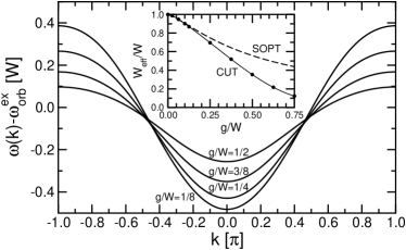
Figure 1: Dispersion $\omega(k)$ of the dressed orbitons for $\omega_{\rm ph}=W$ using the truncation $({{}^{2}V},e\!=\!9)$. Inset: Effective band width $W_{\rm eff}$ as obtained by CUT and by SOPT. For small values of $g$ one has $\delta W_{\rm eff}\propto-g^{2}$ for $W<\omega_{\rm ph}$ and $\delta W_{\rm eff}\propto-g^{4/3}$ for $W=\omega_{\rm ph}$ in 1D.

Figure 2: Effect of the different truncation schemes on the orbiton dispersion $\omega(k)$ for $\omega_{\rm ph}=W$. Upper panel: the difference $\delta\omega(k)=\omega(^{2}\Gamma,e\!=\!9)\,-\,\omega(^{2}V,e\!=\!9)$ at constant extension $e\!=\!9$. Lower panel: $\delta\omega(k)=\omega(^{2}V,e\!=\!7)\,-\,\omega(^{2}V,e\!=\!9)$ at constant structure $S={{}^{2}V}$.

III Method

We choose the CUT approach Głazek and Wilson (1993); Wegner (1994); Knetter and Uhrig (2000); Reischl et al. (2004) because it is an analytical approach which provides an effective model that can be understood more easily. The CUT is defined by

$$\partial_{l}H(l)=[\eta(l),H(l)]$$ (2)

to transform $H(l=0)=H_{0}$ from its initial form to an effective Hamiltonian $H(\infty)$ at $l=\infty$. Here $l$ is a continuous running variable which parametrizes the unitary transformation $U(l)$ yielding $H(l)=U(l)^{\dagger}HU(l)$. The infinitesimal anti-Hermitian generator of the transformation is denoted by $\eta(l)$. The properties of the effective Hamiltonian depend on the choice of the generator.

In this work a quasi-particle-conserving CUT is used which maps the Hamiltonian $H_{0}$ to an effective Hamiltonian $H(\infty)$ which conserves the number of quasi-particlesKnetter and Uhrig (2000); Reischl et al. (2004). This is suggested from the physics of our model. The free orbital wave will be dressed by the interaction with the phononic degrees of freedom. The elementary excitations of the interacting model are orbiton excitations with a cloud of phonons renormalizing the properties of the bare orbital waves.

The following choice for the matrix elements of the infinitesimal generator $\eta$

$$\eta_{i,j}(l)={\rm sgn}\left(q_{i}-q_{j}\right)H_{i,j}(l)$$ (3)

in an eigen basis of $H_{\rm ph}=\omega_{\rm ph}\sum_{i}b^{\dagger}_{i}b^{\phantom{\dagger}}_{i}$ is appropriate. The $q_{i}$ are the eigen values of $H_{\rm ph}$Knetter and Uhrig (2000). Obviously, the flow (2) stops if either $q_{i}=q_{j}$ or $H_{i,j}=0$ for pairs of $i$ and $j$. Given that there is convergence for $l\to\infty$, i.e. $H(\infty)$ exists, this tells us that $H(\infty)$ is block diagonal, i.e. it conserves the phonon number.

The convergence is not as easy to see generally. But assuming an almost diagonal, non-degenerate Hamiltonian with $q_{i}\leq q_{j}\Leftrightarrow H_{i,i}\leq H_{j,j}$ the leading order in the non-diagonal matrix elements fulfills

$$\partial_{l}H_{i,j} = -{\rm sgn}\left(q_{i}-q_{j}\right)(H_{i,i}-H_{j,j})H_{i,j}(l)$$ (4a)

$$= -|H_{i,i}-H_{j,j}|H_{i,j}(l)$$ (4b)

implying convergence according to

$$H_{i,j}\propto\exp(-|H_{i,i}-H_{j,j}|l)\ .$$ (5)

The general derivations of convergence are given in Refs. Mielke, 1998; Knetter and Uhrig, 2000.

The commutators required for the flow (2) are computed using the standard bosonic algebra. The truncation of the proliferating terms in the flow equation will be discussed below. We consider

$$H(\ell) = \sum_{i,n}J_{n}c^{\dagger}_{i+n}c^{\phantom{\dagger}}_{i}+\omega_{\rm ph}\sum_{i}b^{\dagger}_{i}b^{\phantom{\dagger}}_{i}$$

$$+ \sum_{i,n_{1},n_{2}}\left(\Gamma_{n_{1},n_{2}}c^{\dagger}_{i+n_{1}}c^{\phantom{\dagger}}_{i+n_{2}}b^{\dagger}_{i}+{\rm h.c.}\right)$$

$$+ \sum_{i,n_{1},n_{2},n_{3}}V_{n_{1},n_{2}}^{n_{3}}c^{\dagger}_{i+n_{1}}c^{\phantom{\dagger}}_{i+n_{2}}b^{\dagger}_{i+n_{3}}b^{\phantom{\dagger}}_{i}$$

$$+ \sum_{i,n_{j}}\left({}^{2}\Gamma_{n_{1},n_{2}}^{n_{3},n_{4}}c^{\dagger}_{i+n_{1}}c^{\phantom{\dagger}}_{i+n_{2}}b^{\dagger}_{i+n_{3}}b^{\dagger}_{i+n_{4}}b^{\phantom{\dagger}}_{i}+{\rm h.c.}\right)$$

$$+ \sum_{i,n_{j}}{}^{2}V_{n_{1},n_{2}}^{n_{3},n_{4},n_{5}}c^{\dagger}_{i+n_{1}}c^{\phantom{\dagger}}_{i+n_{2}}b^{\dagger}_{i+n_{3}}b^{\dagger}_{i+n_{4}}b^{\phantom{\dagger}}_{i+n_{5}}b^{\phantom{\dagger}}_{i}\ .$$

The only finite amplitudes at $\ell$=0 are $J_{0}(\ell\!=\!0)\!=\!\omega_{\rm orb}^{\rm ex}+\omega_{\rm orb}^{\rm JT}$, $J_{1}(\ell\!=\!0)\!=\!-J/4$, and $\Gamma_{0,0}(\ell\!=\!0)\!=\!2g$. The generator $\eta(\ell)$ is chosen to be

$$\eta(\ell) = \sum_{i,n_{1},n_{2}}\left(\Gamma_{n_{1},n_{2}}c^{\dagger}_{i+n_{1}}c^{\phantom{\dagger}}_{i+n_{2}}b^{\dagger}_{i}-{\rm h.c.}\right)$$

$$+ \sum_{i,n_{j}}\left({}^{2}\Gamma_{n_{1},n_{2}}^{n_{3},n_{4}}c^{\dagger}_{i+n_{1}}c^{\phantom{\dagger}}_{i+n_{2}}b^{\dagger}_{i+n_{3}}b^{\dagger}_{i+n_{4}}b^{\phantom{\dagger}}_{i}-{\rm h.c.}\right)\ .$$

In the following we denote the considered truncations by $(S,e)$ with the structure $S\in\{\Gamma,V,{{}^{2}\Gamma},{{}^{2}V}\}$ and the spatial extension $e$. The structure $S$ is defined by the maximum number of creation and annihilation operators appearing in the flowing Hamiltonian, e.g. $S={{}^{2}V}$ for $H(\ell)$ given in Eq. III. The spatial extension $e$ is defined for a given operator $c^{\dagger}_{i+n_{1}}c^{\phantom{\dagger}}_{i+n_{2}}b^{\dagger}_{i+n_{3}}\ldots b^{\phantom{\dagger}}_{i}$ by the distance between the leftmost and the rightmost local operator, i.e. for $e$=9 only the exchange amplitudes $J_{n}$ with $n\!\in\!\{-4;-3;\ldots;3;4\}$ are finite. We considered $e\!\in\!\{1,3,5,7,9\}$ for the numerical evaluation. We have found that $e$=9 and $S={{}^{2}V}$ is sufficient to obtain numerically stable, accurate results (see below, Figs. 2, 5, and 6).

IV Results

IV.1 Orbiton Dispersion

In Fig. 1, the dispersion of the dressed orbitons is shown for $\omega_{\rm ph}\!=\!W$ using the truncation $({{}^{2}V},e\!=\!9)$. With increasing $g/W$ the effective band width $W_{\rm eff}$ is strongly reduced (see inset). The orbiton becomes dynamically dressed by a phonon cloud enhancing its effective mass. Already for $g/W$=1/2 we find $W_{\rm eff}/W$=0.35 in CUT. In contrast, the approximate perturbative result $W_{\rm eff}/W$=0.56 obtained by SOPT clearly underestimates the reduction of the band width. For $g/W$=3/4 we find $W_{\rm eff}/W$=0.1 in CUT, a factor of 4 smaller than in SOPT. This indicates that for $g\gtrapprox 0.75W$ the excitation may be regarded as ‘local’ for practical purposes, i.e. rather as a vibron than as a propagating orbiton.

The dependence of the orbiton dispersion on the truncation level is depicted in Fig. 2. The upper panel shows the difference $\delta\omega(k)=\omega(^{2}\Gamma,e\!=\!9)\,-\,\omega(^{2}V,e\!=\!9)$, illustrating the dependence on the structure $S$. Clearly, $\delta\omega(k)$ increases with $g$ but remains small ($\delta\omega/W_{\rm eff}<1$%) for all considered values of $g$. The truncation error resulting from the finite spatial extension $e$ of the operators is even smaller, as shown in the lower panel of Fig. 2. This reflects the fact that the physics of the model becomes more local with increasing $g$, hence less extended operators are sufficient to describe the orbiton dispersion. This is underlined by the observation that the truncation error related to the extension $e$ is smaller for $g/W=1/2$ than for $g/W=3/8$.

IV.2 Spectral Properties

For the orbiton line shape, we transform the local orbiton creation operator $\mathcal{O}^{\rm loc}=c_{0}^{\dagger}$ to an effective one by the same CUT as applied to $H_{0}$. We study all terms with one orbiton operator plus up to four phonon operators

$$\mathcal{O}(\ell) = \sum_{r}A_{r}c^{\dagger}_{r}+\sum_{r_{1},r_{2}}\left(B_{r_{1}}^{r_{2}}c^{\dagger}_{r_{1}}b^{\dagger}_{r_{2}}+C_{r_{1}}^{r_{2}}c^{\dagger}_{r_{1}}b^{\phantom{\dagger}}_{r_{2}}\right)$$

$$+ \ldots$$

$$+ \sum_{r_{j}}\left(K_{r_{1}}^{r_{2},r_{3},r_{4},r_{5}}c^{\dagger}_{r_{1}}b^{\dagger}_{r_{2}}b^{\dagger}_{r_{3}}b^{\dagger}_{r_{4}}b^{\dagger}_{r_{5}}+\ldots\right)+{\rm h.c.}\ .$$

Initially, the only finite value is $A_{0}(\ell=0)=1$. Finally, at $T=0$, there are five types of contributions (omitting spatial indices): $c^{\dagger}$, $c^{\dagger}b^{\dagger}$, $c^{\dagger}b^{\dagger}b^{\dagger}$, $c^{\dagger}b^{\dagger}b^{\dagger}b^{\dagger}$, and $c^{\dagger}b^{\dagger}b^{\dagger}b^{\dagger}b^{\dagger}$. For each type we sum the moduli squared of all coefficients, yielding the spectral weights given in Fig. 3.

The sum of all contributions has to equal unity. The inset of Fig. 3 shows that the sum of the five considered contributions is very close to 1 for $g/W\leq 1/2$ so that higher-order terms are indeed not important in this parameter range. For small values of $g/W$, the spectral weight resides almost entirely in the fundamental orbiton band, i.e., the eigen mode is a well-defined orbital wave. With increasing $g/W$ spectral weight is transferred to the orbiton-phonon continua, which reflects the change of the excitation character from an orbital wave to a vibronic excitation with increasing $g$. Already for $g/W$=1/2 the orbiton-plus-one-phonon band dominates the spectrum. This agrees roughly with the result obtained for the local limit of both orbitons and phonons van den Brink (2001).

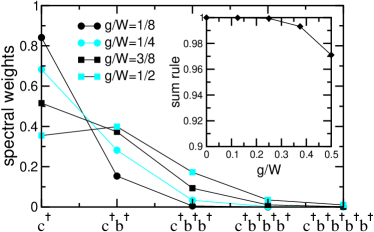
Figure 3: (Color online) Spectral weights of the orbiton quasi-particle band and of the orbiton-plus-$n$-phonon continua ($n$=1-4) for $\omega_{\rm ph}/W=1$ using the truncation $({{}^{2}V},e\!=\!9)$. Inset: The sum of the weights of the five considered contributions obeys the sum rule very well. Lines are guides to the eye only.

Figure 4: The $k$-resolved spectral weight of the orbiton quasi-particle band (top) and of the orbiton-plus-one-phonon sideband (bottom) for $\omega_{\rm ph}\!=\!W$ using the truncation $({{}^{2}V},e\!=\!9)$.

Figure 5: Effect of the truncation on the $k$-resolved spectral weight of the orbiton quasi-particle band for $\omega_{\rm ph}/W=1$. Upper panel: the difference $\delta I=I({{}^{2}\Gamma},e\!=\!9)\,-\,I({{}^{2}V},e\!=\!9)$ at constant extension $e=9$. Lower panel: $\delta I=I({{}^{2}V},e\!=\!7)\,-\,I({{}^{2}V},e\!=\!9)$ at constant structure $S={{}^{2}V}$.

Figure 6: Effect of the truncation on the $k$-resolved spectral weight of the orbiton-plus-one-phonon sideband for $\omega_{\rm ph}/W=1$. Upper panel: the difference $\delta I=I({{}^{2}\Gamma},e\!=\!9)\,-\,I({{}^{2}V},e\!=\!9)$ at constant extension $e=9$. Lower panel: $\delta I=I({{}^{2}V},e\!=\!7)\,-\,I({{}^{2}V},e\!=\!9)$ at constant structure $S={{}^{2}V}$.

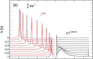
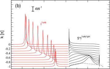
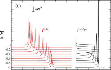
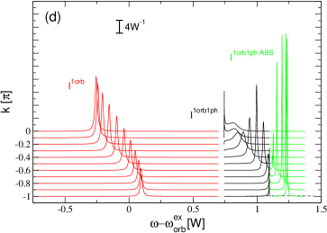
Figure 7: (Color online) Spectral density of one orbiton (red) and the orbiton-plus-one-phonon continuum (black) for $\omega_{\rm ph}/W=1$ using the truncation $({{}^{2}V},e\!=\!9)$. An orbiton-phonon anti-bound state (green) is shown where it has gained substantial weight. (a) $g/W$=1/8. (b) $g/W$=1/4. (c) $g/W$=3/8. (d) $g/W$=1/2. The $\delta$-functions are broadened by $\Gamma=0.01W$. The dashed lines depict the orbiton-plus-one-phonon continuum in SOPT for $k=-\pi$.

Now we turn to momentum ($k$) and frequency ($\omega$) resolved spectral properties. The $k$-resolved spectral weights of the dressed orbiton and of the orbiton-plus-one-phonon continuum are plotted in Fig. 4. The dependence of these two quantities on the truncation level is illustrated in Figs. 5 and 6. Again, the differences between different truncations are small for all considered values of $g$. As mentioned above, the physics becomes more local with increasing $g$, explaining the larger sensitivity on the spatial extension observed for $g/W$=1/8.

The corresponding $k$-resolved spectral densities are shown in Fig. 7. The transfer of spectral weight away from the orbiton band is largest at the Brillouin zone boundary, see top panel of Fig. 4, where the orbiton band is energetically close to the continuum, see Fig. 7a. For small values of $g/W$, the spectral weight ‘leaks’ into the continuum where it appears as a broad hump. For $g/W$=1/8, the results of SOPT and CUT for the line shape and the spectral weight still agree well with each other, see Fig. 7a. With increasing $g/W$, the effective orbiton band width $W_{\rm eff}$ is reduced so that the separation between the orbiton band and the orbiton-plus-one-phonon continuum increases. At the same time, a sharp resonance appears within the continuum, displaying a clear dispersion.

For $g/W$=1/2, the orbiton-plus-one-phonon sector dominates the spectrum, cf. Fig. 3. Its spectral weight is almost independent of $k$, in contrast to the behavior observed for smaller values of $g/W$, see bottom panel of Fig. 4. The relative suppression of the orbiton-plus-one-phonon continuum close to the Brillouin zone boundary reflects the transfer of spectral weight to the orbiton-plus-two-phonon continuum.

IV.3 Anti-Bound State

Interestingly, a very sharp dispersive feature is pushed out of the continuum to higher energies. Because it is built from states with one orbiton and one phonon and because it develops from the scattering states in the continuum, but lying at higher energies, this feature is identified as an anti-bound state (ABS) of one orbiton and one phonon.

The appearance of an ABS is also found in SOPT, though at different energies and with different weights (not shown). It occurs for all momenta and arbitrarily weak couplings $g$ due to the 1D van Hove singularities. In contrast, the sharp resonance seen within the orbiton-phonon continuum at intermediate couplings is totally missed by the SOPT which stays broad and featureless, see dashed lines in Fig. 7.

For $g/W$=1/2 the total dispersion – from the peak maxima in the continuum at $k$=0 to the ABS at $k$=$-\pi$ – is even larger than the renormalized band width $W_{\rm eff}$ of the orbiton band. This surprising result indicates that the dispersion of collective orbital excitations may very well be observed experimentally even for intermediate values of the phonon coupling $g$.

The dispersion of the anti-bound state and of the resonance in the orbiton-phonon continuum comes as a surprise since we started from entirely local phonons. How can an ABS of an orbiton and of an immobile phonon propagate ? Since in our model (1) a single orbiton cannot influence the macroscopic number of phonons we can exclude that some hopping amplitude of the phonons is induced by $g$. Hence we are led to the conclusion that there must be an important momentum-dependent effective interaction between an orbiton and a phonon. A pair of orbiton and phonon undergoes correlated hopping. In the Hamiltonian $H_{0}$ in (1) before the CUT, this hopping can presumably be understood as a virtual process where the orbiton-phonon pair is intermediately de-excited to a single orbiton which can hop. Momentum-dependent matrix elements are certainly also present; but they alone cannot explain the dispersion of the ABS.

In the literature on the Holstein model, the appearance of sharp subbands which are qualitatively similar to our results has been reported for $W$ significantly larger than $\omega_{\rm ph}$ and large values of the coupling constant.Hohenadler et al. (1967); Fehske et al. (2006) However, the identification of the anti-bound state by our CUT approach is essential in order to understand why the dispersion in higher subbands is larger than in the elementary orbiton/polaron band.

V Summary

Our work is intended to provide information on the nature of orbital excitations in the presence of substantial orbiton-phonon coupling in principle. We do not aim at any particular compound. Therefore, we have concentrated on a simplified model in one dimension without hybridization or phonon dispersion. As indicated in the discussion following Eq. (1), we expect that our findings apply qualitatively also to more specific, extended models. In two or three dimensions, the line shape at the band edges will change and the anti-bound state will form only beyond a certain threshold of the orbiton-phonon interaction. The presence of hybridization will imply that the orbiton line shape occurs as a weak feature also in experimental probes coupling directly to the distortions and vice versa. Finally, a finite phonon dispersion will contribute to the mobility of the collective states. In case continua start to overlap, effects of finite life times due to decay will be observable. These points summarize what we expect for the modifications of our findings in real systems.

We investigated the gradual transition from a propagating orbital wave to a ‘local’ vibron with increasing phonon coupling $g$. We found already for intermediate couplings a substantial reduction of the orbiton band width. The orbiton-phonon continuum is not a featureless hump as suggested by second order perturbation theory (Born approximation), but displays a relatively sharp, dispersive resonance and an anti-bound state. For $g/W$=1/2, the orbiton-plus-one-phonon sector carries more spectral weight than the orbiton itself, but it also shows the larger dispersion. Thus the collective character is seen rather in the orbiton-phonon sector than in the fundamental orbiton sector. This may turn out as a major advantage for experiments, since phonons and orbiton-plus-phonon features appear in separate frequency ranges, facilitating the correct assignment. Our results demonstrate that signatures of collective orbital excitations are not limited to compounds in which the phonon coupling $g$ is very small.

We acknowledge fruitful discussion with H. Fehske and G. Khalliulin and the financial support of the DFG in SFB 608 in which this project has been started.

References

- Tokura and Nagaosa (2000) Y. Tokura and N. Nagaosa, Science 288, 462 (2000).
- Khomskii (2005) D. I. Khomskii, Physica Scripta 72, CC8 (2005).
- Khaliullin (2005) G. Khaliullin, Prog. Theor. Phys. Suppl. 160, 155 (2005).
- Jahn and Teller (1937) H. A. Jahn and E. Teller, Phys. Roy. Soc. Lond. A 161, 220 (1937).
- Kugel and Khomskii (1973) K. I. Kugel and D. I. Khomskii, Sov. Phys. JETP 37, 725 (1973).
- Ishihara et al. (2005) S. Ishihara, Y. Murakami, T. Inami, K. Ishii, J. Mizuki, K. Hirota, S. Maekawa, and Y. Endoh, New J. Phys. 7, 119 (2005).
- Saitoh et al. (2001) E. Saitoh, S. Okamoto, K. T. Takahashi, K. Tobe, K. Yamamoto, T. Kimura, S. Ishihara, S. Maekawa, and Y. Tokura, Nature 410, 180 (2001).
- Miyasaka et al. (2005) S. Miyasaka, S. Onoda, Y. Okimoto, J. Fujioka, M. Iwama, N. Nagaosa, and Y. Tokura, Phys. Rev. Lett. 94, 076405 (2005).
- Sugai and Hirota (2006) S. Sugai and K. Hirota, Phys. Rev. B 73, 020409(R) (2006).
- van den Brink (2001) J. van den Brink, Phys. Rev. Lett. 87, 217202 (2001).
- Allen and Perebeinos (1999) P. B. Allen and V. Perebeinos, Phys. Rev. Lett. 83, 4828 (1999).
- Grüninger et al. (2002) M. Grüninger, R. Rückamp, M. Windt, P. Reutler, C. Zobel, T. Lorenz, A. Freimuth, and A. Revcolevschi, Nature 418, 39 (2002).
- Rückamp et al. (2005) R. Rückamp, R. Rückamp, E. Benckiser, M. W. Haverkort, H. Roth, T. Lorenz, A. Freimuth, L. Jongen, A. Möller, G. Meyer, et al., New J. Phys. 7, 144 (2005).
- Głazek and Wilson (1993) S. D. Głazek and K. G. Wilson, Phys. Rev. D 48, 5863 (1993).
- Wegner (1994) F. J. Wegner, Ann. Physik 3, 77 (1994).
- Knetter and Uhrig (2000) C. Knetter and G. S. Uhrig, Eur. Phys. J. B 13, 209 (2000).
- Mielke (1997) A. Mielke, Europhys. Lett. 40, 195 (1997).
- Reischl et al. (2004) A. Reischl, E. Müller-Hartmann, and G. S. Uhrig, Phys. Rev. B 70, 245124 (2004).
- Hohenadler et al. (1967) M. Hohenadler, M. Aichhorn, and W. von der Linden, Phys. Rev. B 68, 184304 (1967).
- Fehske et al. (2006) H. Fehske, A. Alvermann, M. Hohenadler, and G. Wellein, in Polarons in Bulk Materials and Systems with Reduced Dimensionality, edited by G. Iadonisi and J. Ranninger (IOS Press, 2006), Proceedings of the International School of Physics Enrico Fermi Course CLXI, p. 285.
- Mielke (1998) A. Mielke, Eur. Phys. J. B 5, 605 (1998).