Coarse-graining a restricted solid-on-solid model

Abstract

A procedure suggested by Vvedensky for obtaining continuum equations as the coarse-grained limit of discrete models is applied to the restricted solid-on-solid model with both adsorption and desorption. Using an expansion of the master equation, discrete Langevin equations are derived; these agree quantitatively with direct simulation of the model. From these, a continuum differential equation is derived, and the model is found to exhibit either Edwards-Wilkinson or Kardar-Parisi-Zhang exponents, as expected from symmetry arguments. The coefficients of the resulting continuum equation remain well-defined in the coarse-grained limit.

I Introduction

Driven, non-equilibrium interfaces have received much attention in recent years. Various models have been used to describe such systems. hhz ; barabasi . These models may usually be assigned to one of a small number of universality classes, each characterised by a set of scaling exponents. To each universality class corresponds a continuum Langevin equation; such an equation may therefore be identified for each lattice model if the exponents are known, for example, from kinetic Monte Carlo (KMC) simulations. This procedure, however, faces difficulties when crossover effects are important kotrlsmil . To overcome this, Vvedensky vved03a has suggested using a combination of an expansion of the master equation vk ; fk ; vzl and the dynamic renormalisation group (DRG) fns ; kpz to coarse-grain the resulting description, thereby directly obtaining a continuum Langevin equation in the large-scale, long-time limit. This program is a particular realization of a program suggested by Anderson pwa .

In this paper we implement this procedure for a restricted solid-on-solid (RSOS) model with both adsorption and desorption. The master equation is expanded to obtain a set of discrete Langevin equations; these are then numerically integrated and compared to direct KMC simulations of the model, with which they are found to be in quantitative agreement. In the up/down symmetric case, an ad hoc procedure and the DRG both lead to the Edwards-Wilkinson (EW) equation

$$\frac{\partial}{\partial t}\phi(x,t)=\nu_{2}\frac{\partial^{2}}{\partial x^{2}}\phi(x,t)+\sqrt{D}\eta(x,t)$$ (1)

as the macroscopic description of the model; here, $\eta$ is a zero-average Gaussian noise field with unit variance. For the asymmetric case, DRG arguments lead to the Kardar-Parisi-Zhang (KPZ) equation,

$$\frac{\partial}{\partial t}\phi(x,t)=\nu_{2}\frac{\partial^{2}}{\partial x^{2}}\phi(x,t)+\lambda_{2}\left(\frac{\partial}{\partial x}\phi(x,t)\right)^{2}+\sqrt{D}\eta(x,t)$$ (2)

as the coarse-grained description. This is consistent with symmetry arguments and simulations kk . The coefficients of the coarse-grained continuum equations remain well-defined in the macroscopic limit.

II The model

The model is a simple generalisation of the RSOS model introduced by Kim and Kosterlitz kk , and a special case of that introduced by Hinrichsen et al hlmp . It is described (in one dimension for simplicity) by a vector $\mathbf{h}(t)$ of $L$ time-dependent, integer-valued heights $h_{i}(t)$, $i=1,2,\dots,N$; time is also a discrete variable. The dynamical evolution is given by the following rules: At each time step, an integer $1\leq i\leq L$ is randomly chosen; with probability $p$ the height $h_{i}$ is increased by 1, and with probability $q$ attempt it is decreased by 1, provided that the resulting configuration does not violate $|h_{i}-h_{i\pm 1}|\leq 1$. Finally, periodic boundary conditions are imposed. The allowed transitions, together with the associated probabilities (equivalently, the rates) are shown in fig. 1.

Figure 1: Allowed transitions and associated transition rates.

The transition rate from configuration $\mathbf{h}$ to $\mathbf{h}+\mathbf{r}$ is given by

$$\begin{split}W(\mathbf{h};\mathbf{r})=\sum_{i}\Bigg{[}&\Big{\{}q\delta(r_{i}-1)\theta(\Delta^{+}h_{i})\theta(-\Delta^{-}h_{i})\\ &+p\delta(r_{i}+1)\theta(-\Delta^{+}h_{i})\theta(\Delta^{-}h_{i})\Big{\}}\mathcal{F}_{i}\Bigg{]},\end{split}$$ (3)

with $\mathcal{F}_{i}=\prod_{j\neq i}\delta(r_{j})$, the discrete derivatives $\Delta^{\pm}h_{i}=\pm\left(h_{i\pm 1}-h_{i}\right)$, and

$$\theta(x)=\begin{cases}1,&x\geq 0\\ 0,&x<0,\end{cases}$$ (4)

for integer (or zero) $x$. The temporal evolution of the probability density $P(\mathbf{h},t)$ is given by the master equation

$$\begin{split}\frac{\partial}{\partial t}P\left(\mathbf{h},t\right)=\int\mathrm{d}^{L}r\,&\Big{[}W\left(\mathbf{h}-\mathbf{r};\mathbf{r}\right)P\left(\mathbf{h}-\mathbf{r},t\right)\\ &\qquad-W\left(\mathbf{h};\mathbf{r}\right)P\left(\mathbf{h},t\right)\Big{]}.\end{split}$$ (5)

In Ref. pk , the special case $q=1$, $p=0$ is studied, and the KPZ equation derived as the coarse-grained description. However, the treatment of Ref. pk leads to ill-defined coefficients precisely in the coarse-grained limit. In particular, the authors find the coarse-grained description to be eqn. (2) with $\nu_{2}$, $\lambda_{2}$ and $D$ proportional to different powers of a parameter, $a$, which controls the degree of coarse-graining; indeed, their results are valid as $a\rightarrow 0$. Such a problem does not arise in our approach.

III A variant of the van Kampen expansion

An often-used method for deriving Fokker-Planck equations for stochastic processes is the van Kampen expansion vk ; fk ; vzl . The method as described in vk ; fk is not directly applicable to systems such as the RSOS model because it requires a small parameter, $1/\Omega$, in which to expand. In effect, it assumes the existence of a macroscopic law along with stochastic corrections to it, the relative size of which is controlled by the expansion parameter vk . In stochastic growth models, this is not the case; it is impossible to separate the time evolution into deterministic and stochastic parts: the stochastic evolution is all there is. A more extended discussion of this point may be found in Refs. thesis ; christophalvin , where it is shown that eqn. (5) may nevertheless be approximated by a Fokker-Planck equation, which corresponds to the Itô Langevin equation

$$\frac{\mathrm{d}}{\mathrm{d}t}h_{i}=K^{(1)}_{i}(\mathbf{h})+\sqrt{K^{(2)}_{ij}(\mathbf{h})}\,\eta_{j}(t)$$ (6)

where summation over repeated indices is implied and the jump moments are defined by

$$K^{(n)}_{i_{1}\dotsi_{n}}(\mathbf{h})=\int\mathrm{d}\mathbf{r}\,r_{i_{1}}\dots r_{i_{n}}W(\mathbf{h};\mathbf{r}).$$

Eqn. (6) is essentially a set of simultaneous coupled Langevin equations. Obtaining a continuum version is conceptually similar to the (inverse of the) method of lines used to solve partial differential equations. However, in the case of discrete interface models, the jump moments $K^{(n)}$ contain non-analytic step functions which necessitate a regularisation procedure. This is done in the next section.

IV Discrete Langevin equations

To apply eqn. (6), the first two jump moments are needed. These can be calculated from $W$ given by eqn. (3) and are

$$K^{(1)}_{i}(\mathbf{h}) =q\,\theta(\Delta^{+}h_{i})\theta(-\Delta^{-}h_{i})-p\,\theta(-\Delta^{+}h_{i})\theta(\Delta^{-}h_{i})$$ (7a)

and

$$K^{(2)}_{ij}(\mathbf{h}) =\left[q\,\theta(\Delta^{+}h_{i})\theta(-\Delta^{-}h_{i})+p\,\theta(-\Delta^{+}h_{i})\theta(\Delta^{-}h_{i})\right]\delta_{ij},$$ (7b)

where $\delta_{ij}$ is a Kronecker delta.

Eqns. (7a) and (7b) are not completely specified by the lattice transition rules of sec. II, but must be extended to non-integer values of the $h_{i}$. Furthermore, in deriving eqn. (6), the implicit assumption that $W(\mathbf{h};\mathbf{r})$ is analytic in $\mathbf{h}$ was made, which in turn implies that the extension of $\theta(x)$ to non-integers must be differentiable. This continuation of the $K^{(n)}$ to noninteger arguments is known as regularisation vzl ; nagatani ; vved03a ; vved03b . We choose the representation of $\theta$ given by

$$\theta(x)=\lim_{\Delta\rightarrow 0^{+}}\theta_{\Delta}(x),$$ (8)

where, following nagatani ; vved03a ; vved03b ,

$$\theta_{\Delta}(x)=\frac{\Delta}{a}\ln\left[\frac{\exp\left((x+a)/\Delta\right)+1}{\exp\left(x/\Delta\right)+1}\right].$$ (9)

The parameter $a$ is the value of $x$ below which $\theta(x)=0$ and must therefore satisfy $0<a<1$ in order to agree with the lattice rules; it is otherwise free at this stage. $\Delta$ is effectively a “smoothing” parameter, and $\theta_{\Delta}$ is an analytic function of $x$ at the origin for all $\Delta>0$. More details may be found in vved03a .

In some cases, such as the Wolf-Villain model analysed in christophalvin , the lattice rules can be used to infer the value of $a$. Here, simple arguments thesis show that $a=0$ leads to a discontinuous (non-analytic) dependence of $K^{(1)}(\mathbf{h})$ on $\mathbf{h}$; this is against the spirit of the model, so $a\neq 0$. Unfortunately, the argument cannot fix the exact value; this must be determined by comparing the results of numerical integration of eqn. (6) to simulations of the lattice model. Accordingly, fig. 2

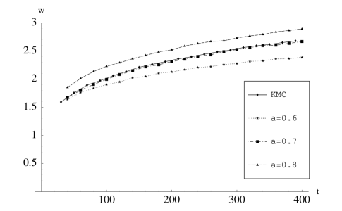
Figure 2: Variation of the evolution of the interfacial width with time for three values of $a$, as well as KMC simulation; $q=1$ and $p=0$, $L=100$. Both KMC and stochastic integration results averaged over 2000 runs.

shows a plot of $w$ against $t$ for $L=100$ with $q=1$ and $p=0$; results from a KMC simulation and numerical integration of the Langevin equations for each of $a=0.6$, $a=0.7$ and $a=0.8$ are presented. It is evident that $a\approx 0.7$ gives a result that agrees closely with the KMC simulation. To test this agreement in the case $q=p=0.5$, we simulate a system of size $L=1000$; fig. 3 shows the early-time behaviour. It again shows that $a\approx 0.7$ gives the best agreement between KMC simulations and the stochastic formulation.

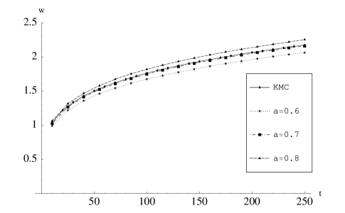
Figure 3: Early-time behaviour of the width for $L=1000$ and $q=p=0.5$ Both KMC and stochastic integration results averaged over 1000 runs.

In conclusion, the system of discrete Langevin equations with the choice $\approx 0.7$ gives quantitatively the same results as the original model.

V The continuum limit

The continuum (coarse-grained) limit of the symmetric case $q=p$ may be taken using a simple ad hoc method, which is direct but physically opaque and cannot be extended to the asymmetric case. The DRG is necessary to analyse the full model; it is considerably more general and conceptually clear, but correspondingly more complicated to carry out. The analysis presented in this section confirms the results of symmetry arguments and constitutes the final step in the identification of the SDE corresponding to the RSOS model.

V.1 Ad hoc approach

Using the regularisation of sec. IV, the step functions may be expanded about $x=0$ as

$$\theta_{\Delta}(x)=\sum_{n=0}^{\infty}b_{n}(\Delta)x^{n}.$$ (10)

Replacing the set $h_{i}(t)$ by a function of a continuous argument $x$, $\phi(x,t)$ (which coincides with $h_{i}(t)$ for $x=i$), and expanding the discrete derivatives transforms the discrete set of SDEs of eqn. (6) into a (partial) stochastic differential equation for $\phi(x,t)$.

By using power counting arguments (see thesis for details), we find that the relevant terms in this equation are, at most,

$$\frac{\partial\phi}{\partial t}=\nu_{2}\frac{\partial^{2}\phi}{\partial x^{2}}+\nu_{4}\frac{\partial^{4}\phi}{\partial x^{4}}+\nu_{6}\frac{\partial^{6}\phi}{\partial x^{6}}+\kappa_{13}\frac{\partial\phi}{\partial x}\frac{\partial^{3}\phi}{\partial x^{3}}+\lambda_{2}\left(\frac{\partial\phi}{\partial x}\right)^{2}+\lambda_{13}\frac{\partial}{\partial x}\left(\frac{\partial\phi}{\partial x}\right)^{3}+\kappa_{22}\left(\frac{\partial^{2}\phi}{\partial x^{2}}\right)^{2}+\sqrt{D}\eta,$$ (11)

where $\eta$ is gaussian noise with unit variance and the coefficients may be found explicitly as functions of the $b_{n}$. The coefficients $\nu_{2},\nu_{4},\nu_{6},\lambda_{13}$ and $D$ are proportional to $q+p$, while the rest are proportional to $q-p$; this is consistent with arguments based on up/down reflection symmetry.

In the symmetric case $q=p$, the only surviving terms are given by $\nu_{2}=12\nu_{4}=360\nu_{6}=b_{0}b_{1}$, $\lambda_{13}=(3b_{0}b_{3}+b_{1}b_{2})/3$ and $D=1$. The coefficients $b_{n}$ may be found explicitly from eqn. (9). These satisfy the following inequality :

$$b_{n}(\Delta)\leq\frac{A_{n}(\Delta)}{\Delta^{n-1}},$$ (12)

where $A_{n}\rightarrow\mathrm{const}$ as $\Delta\rightarrow 0^{+}$.

A simple scaling approach would involve rescaling space, time and the field as $x\rightarrow\epsilon x$, $t\rightarrow\epsilon^{z}t$ and $\phi\rightarrow\epsilon^{\alpha}\phi$, respectively, followed by taking the limit $\epsilon\rightarrow 0^{+}$. Instead, following vved03a ; vved03b , we will take the two limits $\epsilon\rightarrow 0$ and $\Delta\rightarrow 0$ together. Putting $\Delta=\epsilon^{\delta}$ with $\delta>0$ to be determined, the limit $\epsilon\rightarrow 0^{+}$ is well-defined only if $z=2$, $\alpha=1/2$ and $\delta=1/2$. The space-time scaling is diffusive (EW), while the value of $\delta$ has no direct physical significance. At the limit, the only surviving terms are the $\nu_{2}$ term and the noise; all the others vanish. We therefore conclude that the coarse-grained limit of the symmetric RSOS model is the EW equation .

Unfortunately, this direct coarse-graining procedure cannot be applied to the asymmetric case. In the next section, both the symmetric and asymmetric version of the model are studied using DRG arguments.

V.2 Dynamic renormalisation group

An equation corresponding to the limit of eqn. (11) for $q=p$ has previously been analysed by das Sarma and Kotlyar dsk ; however, the DRG flow equation for $\lambda_{13}$ is not derived in Ref. dsk .

For this section, eqn. (11) will be generalised to $d$ dimensions in the obvious way. Defining $K_{d}=S_{d}/(2\pi)^{d}$, $S_{d}=2\pi^{d/2}/\Gamma\left(d/2\right)$ and $g=\lambda_{13}D/\nu_{2}^{2}$, we find, to first order in $g$ (which plays the role of an effective coupling constant)

$$\frac{\mathrm{d}\nu_{2}}{\mathrm{d}l} =\nu_{2}\left(z-2+\frac{1}{2}gK_{d}\frac{d+2}{d}\right),$$ (13a)

$$\frac{\mathrm{d}\lambda_{13}}{\mathrm{d}l} =\lambda_{13}\left(2\alpha+z-4-\frac{1}{2}gK_{d}\frac{d^{2}+6d+20}{d(d+2)}\right),$$ (13b)

$$\frac{\mathrm{d}D}{\mathrm{d}l} =D\left(z-d-2\alpha\right)$$ (13c)

(the non-renormalisation of $D$ is a well-known consequence of the fact that the deterministic part of the equation is conservative). The flow equation for $g$ is given by

$$\frac{\mathrm{d}g}{\mathrm{d}l}=-g\left(d+g\frac{K_{d}}{2d(d+2)}\left(3d^{2}+14d+28\right)\right).$$ (14)

For any positive $g\left(l\!=\!0\right)$ (which is the case here thesis ), $g=0$ is an attractive fixed point . This fixed point corresponds to $z=2$ and $\alpha=(2-d)/2$, with $\lambda_{13}=0$, that is, it is the fixed point of the EW universality class, in agreement with the ad hoc approach of the previous section (as well as symmetry arguments and computer simulations).

Application of the full machinery of the DRG to eqn. (11) is unnecessary because definite conclusions may be reached by inspection of the equation. In terms of the Fourier transform of $\phi(x,t)$, which we denote by the same symbol $\phi(\mathbf{k},\omega)$, eqn. (11) (generalised to $d$ dimensions) becomes

$$G_{0}(\mathbf{k},\omega)\phi(\mathbf{k})=\eta(\mathbf{k},\omega)+\int_{\mathbf{q},\Omega}M_{2}(\mathbf{q},\mathbf{k}-\mathbf{q})\phi(\mathbf{q})\phi(\mathbf{k}-\mathbf{q})+\int_{\mathbf{q},\mathbf{q}^{\prime}\,\Omega,\Omega^{\prime}}\left[M_{3}(\mathbf{k},\mathbf{k}-\mathbf{q}-\mathbf{q}^{\prime},\mathbf{q},\mathbf{q}^{\prime})\phi(\mathbf{q})\phi(\mathbf{q}^{\prime})\phi(\mathbf{k}-\mathbf{q}-\mathbf{q}^{\prime})\right].$$ (15)

where the argument $\omega$ has been suppressed for $\phi$, the bare response function is

$$G_{0}(\mathbf{k},\omega)=\nu_{2}k^{2}-\nu_{4}k^{4}+\nu_{6}k^{6}-i\omega,$$

and the two vertices are

$$M_{3}\left(\mathbf{k}_{1},\mathbf{k}_{2},\mathbf{k}_{3},\mathbf{k}_{4}\right)=\lambda_{13}\left[\mathbf{k}_{1}\cdot\mathbf{k}_{4}\right]\left[\mathbf{k}_{2}\cdot\mathbf{k}_{3}\right]$$ (16)

and

$$\begin{split}M_{2}\left(\mathbf{k}_{1},\mathbf{k}_{2}\right)=&-\lambda_{2}\left(\mathbf{k}_{1}\cdot\mathbf{k}_{2}\right)+\kappa_{22}(\mathbf{k}_{1})^{2}(\mathbf{k}_{2})^{2}\\ &+\frac{1}{2}\kappa_{13}(\mathbf{k}_{1}\cdot\mathbf{k}_{2})\left[(\mathbf{k}_{1})^{2}+(\mathbf{k}_{2})^{2}\right].\end{split}$$ (17)

In the long-wavelength limit $k\rightarrow 0$ the 2-vertex of eqn. (17) will be dominated by the $\lambda_{2}$ (KPZ) term, with the $\kappa_{ij}$ terms playing the role of higher-order corrections. Similarly, the 3-vertex is of higher order than the KPZ term; in addition, it has been shown to be irrelevant previously. Therefore, the KPZ term $\lambda_{2}$ determines the universality class of the model.

Since $\lambda_{2},\kappa_{ij}\propto(q-p)$, if $q=p$ then $M_{2}=0$ initially. If only vertices with an odd number of legs are present in the bare (unrenormalized) equation then vertices with an even number of vertices cannot be produced under renormalization. Therefore, if $q=p$ the KPZ term is not present and the coarse-grained dynamics of the system is described by the EW equation. If $q\neq p$, the dynamics is described by the KPZ equation. This result is consistent with symmetry arguments and simulation results thesis .

VI Summary

We have implemented a procedure suggested by Vvedensky (and in more general terms by Anderson pwa ) to obtain macroscopic equations from microscopic models.

Discrete Langevin equations are first derived and numerically integrated; they are found to be in quantitative agreement with KMC simulations of the underlying model. Next, these equations are expanded leading to a continuum Langevin equation, from which it is shown that the coarse-grained description of the model is the KPZ equation with the coefficient of the nonlinear term $\lambda_{2}$ vanishing in the symmetric case, so that the EW equation is obtained. The coefficients appearing in the equation are well-defined in the coarse-grained limit.

The advantage of this procedure over the identification of the universality class by direct determination of the exponents from simulations is that slow convergence to the asymptotic regime is not a problem. In addition, the DRG approach allows, in principle, investigation of crossover effects (although this has not been pursued here). Application of this procedure to other models would be a fruitful area for the future.

- (1) T. Halpin-Healey and Y.-C. Zhang, Phys. Rep. 254 215 (1995)
- (2) A.-L. Barabási and H. E. Stanley Fractal Concepts in Surface Growth (Cambridge University Press, Cambridge, 1995)
- (3) M. Kotrla and P. Smilauer, Phys. Rev. B 53 13777 (1996)
- (4) D. D. Vvedensky, Phys. Rev. E 67 025102 (2003)
- (5) D. D. Vvedensky, A. Zangwill, C. N. Luse and M. R. Wilby, Phys. Rev. E 48 852 (1993)
- (6) N. G. van Kampen, Stochastic Processes in Physics and Chemistry (North Holland, Amsterdam, 1992)
- (7) R. F. Fox and J. Keizer, Phys. Rev. A 43 1709 (1991)
- (8) D. Forster, D. R. Nelson and M. J. Stephen, Phys. Rev. A 16 732 (1977)
- (9) M. Kardar, G. Parisi and Y.-C. Zhang, Phys. Rev. Lett. 56 889 (1986)
- (10) P. W. Anderson, Basic Notions of Condensed Matter Physics, Benjamin/Cummings (California, 1984), p. 212
- (11) J. M. Kim and J. M. Kosterlitz, Phys. Rev. Lett 62, 2289 (1989)
- (12) H. Hinrichsen, R. Livi, D. Mukamel and A. Politi, Phys. Rev. Lett. 79 2710 (1997)
- (13) K. Park and B. Kahng, Phys. Rev. E 51 796 (1995)
- (14) A. Lazarides, PhD Thesis, Department of Mathematics, Imperial College London (2005)
- (15) C. Baggio, A. L.-S. Chua, C. A. Haselwandter and D. D. Vvedensky, Phys. Rev. E 72 051103 (2005)
- (16) D. D. Vvedensky, Phys. Rev. E 68 010601 (2003)
- (17) T. Nagatani, Phys. Rev. E 58 700 (1998)
- (18) S. Das Sarma and R. Kotlyar, Phys. Rev. E 50 4275 (1994)