Relationship between Fragility, Diffusive Directions and Energy Barriers in a Supercooled Liquid

Abstract

An analysis of diffusion in a supercooled liquid based solely in the density of diffusive directions and the value of energy barriers shows how the potential energy landscape (PEL) approach is capable of explaining the $\alpha$ and $\beta$ relaxations and the fragility of a glassy system. We find that the $\beta$ relaxation is directly related to the search for diffusive directions. Our analysis shows how in strong liquids diffusion is mainly energy activated, and how in fragile liquids the diffusion is governed by the density of diffusive directions. We describe the fragile-to-strong crossover as a change in the topography of the PEL sampled by the system at a certain crossover temperature $T_{\times}$.

, ,

1 Introduction

The study of slow dynamics in disorder systems and, in particular, the study of the glass transition in supercooled liquids is a topic of considerable interest in condensed matter physics. In general, liquids are divided in two different classes depending on the properties of their glass transitions, strong and fragile [1]. Strong liquids experience a gentle increase in the relaxation upon cooling, often according to the Arrhenius law, close to the glass transition temperature $T_{g}$. On the other hand, fragile liquids, experiment a sharp rise of the viscosity, increasing by several orders of magnitude in a very narrow interval of temperature close to $T_{g}$. The glass transition temperature is not related to any dynamical transition and is experimentally defined as the one where the value of the viscosity is $10^{13}$ P. For strong liquids, nothing special happens close to $T_{g}$ and the glass transition shows a conventional behavior where no transition may be defined. However, fragile systems seem to present a divergence behavior close to $T_{g}$ indicating that some kind of new dynamical mechanism may be responsible for the onset of the glassy phase. Theoretical attempts conducted to study this possible new transition have been mainly focused in two different approaches: the mode coupling theory (MCT) [2], and the potential energy landscape (PEL) [3].

MCT studies structural arrest in supercooled liquids as a purely dynamic singularity happening as a result of a feedback between shear-stress, diffusion and viscosity. The idealized MCT predicts structural arrest to take place at a temperature $T_{\mbox{\scriptsize MC}}>T_{g}$ [4, 5]. To restore ergodicity below $T_{\mbox{\scriptsize MC}}$ additional hopping or activated mechanism have been introduced into the theory [6], avoiding the kinetic singularity. MCT accurately describes important aspects of relaxation dynamics in liquids above their melting temperatures, in particular, the behavior of the intermediate scattering function and the $\alpha$ and $\beta$ relaxations. The $\beta$ relaxation plateau is related to the time expended by the particle to break the cage formed by neighboring particles. The accuracy of the MCT predictions above $T_{g}$ has been verified experimentally and using computer simulations [7, 8, 9].

The potential energy landscape (PEL) approach has been studied using the concept of an inherent structure (IS) [10] (i.e., the configurations at the local minimum of the system’s potential energy). Several numerical and theoretical studies have provided evidence of a relation between the dynamics of the supercooled liquid and the PEL. It was found that correlation functions display stretching in time in the same temperature range in which the systems explores local minima of the PEL with deeper and deeper energy [11, 12], a thermodynamic description of the supercooled liquid was performed in terms of the IS configurational entropy [13], fragility was related to properties of the PEL [14] and the diffusion process was analyzed in terms of the visited inherent structures [15].

There was no connection between both theories (MCT and PEL). Basically there has not been a clear definition of $T_{\mbox{\scriptsize MC}}$ from the potential energy landscape point of view and a precise landscape-based definition of hopping and activated dynamics has been lacking [16]. This situation has recently changed due to the instantaneous normal mode approach to the PEL [17]. This approach relates the diffusive processes to the number of accessible paths in the multidimensional energy landscape [18, 19, 20]. In particular, a key point is the temperature dependence of the fraction of negative eigenvalues of the Hessian calculated at the saddle points of the PEL [21, 22]. It was found that this fraction approaches zero at $T_{\mbox{\scriptsize MC}}$, but is appreciable at larger temperatures. Since the negative eigenvalues correspond to diffusive directions on the PEL, the following scenario was proposed for the dynamics of supercooled liquids close to the glass transition: For $T>T_{\mbox{\scriptsize MC}}$ the system lies close to saddles in the configuration space and the relevant dynamic process is a diffusion among the saddle points along paths at almost constant potential energy, where there is no need to overcome any energetic barrier (“border dynamics”). That implies that the factors impeding free diffusion of the particles are related to finding these paths (entropic factors), rather than due to energetic factors. However, below $T_{\mbox{\scriptsize MC}}$, there are few paths available and diffusion is dominated by hopping processes allowing the system to evolve from minimum to minimum (minimum-to-minimum dynamics). This implies that a sharp slowing down on the dynamics should take place close to $T_{\mbox{\scriptsize MC}}$ if the energetic barriers to be crossed by the system are high enough [23].

2 Analytic approach to the PEL

To check if this proposed mechanism is correct we are going to study the problem analytically, relating the properties of the PEL—the density of diffusive directions and value of the energy barriers—directly to the fragile and strong characteristics of supercooled liquids, and to the $\alpha$ and $\beta$ relaxations predicted by MCT.

We consider particles following a Brownian motion in three-dimensional space. In the absence of any other kind of interaction the mean square displacement is given by

$$\langle r^{2}(t)\rangle=6T[t-(1-e^{-t})].$$ (1)

Here we set the Boltzmann constant $k=1$, and take the particle masses $m=1$. For very short times ($t\ll 1$), the particles behave as free particles $\langle r^{2}(t)\rangle=3Tt^{2}$, and for longer periods of time ($t\gg 1$) the particles behave as diffusive particles in a random walk $\langle r^{2}(t)\rangle=6Tt$.

For particles in supercooled liquids such as Lennard-Jones systems, silica or water, the evolution is much more complicated due to non-trivial interactions among particles. These non-trivial interactions produce a very complicated energy landscape, making analytical results very difficult to obtain. However, a lot of information about these energy landscapes has been obtained using powerful numerical techniques such as Molecular Dynamics or Monte Carlo simulations. In particular, it has been proposed that the density of diffusive directions with temperature, $k(T)$, follows a power law [21]

$$k(T)=A(T-T_{\mbox{\scriptsize MC}})^{\gamma}.$$ (2)

The typical value $\Delta E$ of the energy barriers in hopping processes close to the mode coupling critical temperature, has been determined for different models [23, 24]. In all cases it has been found that a good approximation is given by

$$\Delta E\approx 10T_{\mbox{\scriptsize MC}}.$$ (3)

For long enough time (we consider a time $t$ to be long enough if $t>1$), the diffusion of a particle is no longer free, making the total system to evolve over the multidimensional PEL. From a thermodynamic point of view the diffusion of the particle takes place if the direction chosen on the PEL turns to be a diffusive one, or if the barrier is low enough to be overcome by means of an activated process. Considering Eqs. (2) and (3), the probability of diffusion of the particle at a temperature T from a time $t>1$ to a time $t+1$ is given by

$$P_{\mbox{\scriptsize diff}}=A(T-T_{\mbox{\scriptsize MC}})^{\gamma}+[1-A(T-T_{\mbox{\scriptsize MC}})^{\gamma}]e^{-\Delta E/T}.$$ (4)

Considering $P_{\mbox{\scriptsize diff}}$, it is possible to relate the total value of the mean square displacement $\langle R^{2}(t)\rangle$ (at time $t>1$) with the value of the random walk diffusion $\langle r^{2}(t)\rangle$ by

$$\langle R^{2}(t)\rangle=\sum_{i=1}^{t}{t-1\choose i-1}\langle r^{2}(i)\rangle P_{\mbox{\scriptsize diff}}^{i-1}(1-P_{\mbox{\scriptsize diff}})^{t-i}.$$ (5)

If $t<1$ the diffusion is the one given by a random walk, $\langle R^{2}(t)\rangle=\langle r^{2}(t)\rangle$.

3 Results for $\langle R^{2}(t)\rangle$

Next, we study $\langle R^{2}(t)\rangle$ from Eq. (5) for four different cases. Our standard case is going to be a binary mixture Lennard-Jones (BMLJ) system with density $\rho=1.2$, as the one studied in ref.[21] for which $T_{\mbox{\scriptsize MC}}=0.435$, $\gamma=0.94$ and $A\approx 0.05$. We will study four cases.

• Case (a): We consider the simplest system where only Brownian motion is present and there is no effect of the PEL. We take $k(T)=1$, implying that any direction chosen by the system is going to be a diffusive one.

• Case (b): The second system considered has a larger density of diffusive directions that the one studied in [21]. To do so we take $A\approx 0.5$. In this particular case $k(T)=1$ for $T>2.5$.

• Case (c): We consider the standard case from ref.[21] where $k(T)\not=1$ for every $T$ in this study.

• Case (d): We consider a case where there are no diffusive directions $A=0\Rightarrow k(T)=0$.

Results are presented in Fig. 1 For temperatures ranging from $T=5$ to $T=0.4386$. A clear relation between the $\beta$ relaxation time and the density of diffusive directions in the system, $k(T)$, is found in Fig. 1. In Case (a) all directions are diffusive and particles do not expend any $\beta$ relaxation time searching for a diffusive direction to scape, that is the reason why there is no plateau in Fig. 1(a). On the contrary, in Case (d), there are no diffusive directions and the particle expends a long time in the $\beta$ relaxation plateau. The only possible diffusion mechanism to scape from this plateau is by an activated process to overcome the $\Delta E$ barrier. So the $\beta$ relaxation time may be interpreted in terms of the PEL as a “search” for diffusive directions. This mechanism should be equivalent to the one described in the MCT where the particles “search” for directions to scape from the cage formed by surrounding particles.

Figure 1: $\ln\langle R^{2}(t)\rangle$ vs. $\ln(t)$ obtained from Eq. (5) for temperatures (from top to bottom) $T=5$, 4, 3, 2, 1, 0.8, 0.6, 0.55, 0.5, 0.475, 0.466, 0.454, 0.444, and 0.439. The values of the parameters are $\gamma=0.94$, $T_{\mbox{\scriptsize MC}}=0.435$, $\Delta E=10T_{\mbox{\scriptsize MC}}$ and (a)$k(T)=1$, (b)$A\approx 0.5$, (c)$A\approx 0.05$ and (d)$A=0$.

4 Results for $D(T)$

Once $\langle R^{2}(t)\rangle$ is known it is possible to determine the diffusion coefficient $D(T)$ as a function of temperature, considering that a straight line, with unit slope, fitted to the long time behavior of data in Fig. 1, intersects a vertical line at $\ln(t)=0$ at a height $\ln(6D)$. To study what is the mechanism in the PEL leading to the behavior of a supercooled liquid as strong or fragile, we study three different cases.

• Case (a): We study a system with no diffusive directions, where the only possibility for the system to diffuse is an activated process to overcome the energetic barrier $\Delta E\simeq 10T_{\mbox{\scriptsize MC}}$. We consider again a value $A=0\Rightarrow k=0$.

• Case (b): We consider the opposite case, where no activation process is available (since the energy barriers are extremely high) and the only diffusion mechanism is the search for diffusive directions. In order to study a system like that we take $\Delta E\simeq 10^{5}T_{\mbox{\scriptsize MC}}$ and $A\approx 0.05$.

• Case (c): Finally we consider the Binary Lennard Jones system considered in [21] where both diffusive mechanisms are available.

Results are presented in Fig. 2. We plot $\ln(6D)$ vs. $1/T$ in Fig. 2(a) and $\ln(6D)$ vs. $\ln(T-T_{\mbox{\scriptsize MC}})$ in Fig. 2(b). Note how Case (a) clearly shows a linear (Arrhenius behavior), typical of a strong liquid. Nothing special happens when $T=T_{\mbox{\scriptsize MC}}$, since the mechanisms of diffusion are always the same (activated processes). On the contrary Case (b) presents the typical behavior of a fragile liquid predicted by MCT. In this case, the transition to a glassy state at $T=T_{\mbox{\scriptsize MC}}$, is a singular one. Since the only mechanism of diffusion are the diffusive directions and those are equal to zero at $T=T_{\mbox{\scriptsize MC}}$ the system gets trapped in a glass state by dynamical arrest. Note how the barrier must be very high to get a really slowing down in the dynamics, making any kind of hopping impossible. This result agrees with predictions made in [23]. If the energy barriers are not high enough we are in Case (c) and we have a transition from strong to fragile behavior at $T=T_{\mbox{\scriptsize MC}}$ as the one predicted by [25] and observed numerically in [26]. Note how Case (c) is almost identical to Case (b) when the temperatures are far from $T_{\mbox{\scriptsize MC}}$ clearly indicating that the mechanisms of diffusion are governed mostly by “border dynamics,” that is, by evolution of the system through the diffusive direction of the PEL. However for $T<T_{\mbox{\scriptsize MC}}$, Case (c) behaves like Case (a), which means that the mechanisms of diffusion are now governed by activated processes to overcome the $\Delta E$ energy barriers. Case (c) is a clear example of crossover from “border dynamics” to “minimum-to-minimum dynamics.”

Figure 2: Figure 2(a) shows $\ln(6D)$ vs. $1/T$. Dashed line is a liner fit to the data for Case (a), dotted line marks the value $T=T_{\mbox{\scriptsize MC}}$. Figure 2(b) shows $\ln(6D)$ vs. $\ln(T-T_{\mbox{\scriptsize MC}})$. Dashed line is a liner fit to the data for Case (b). The values of the parameters in the different cases are Case (a) $\Delta E=10T_{\mbox{\scriptsize MC}}$, $A=0$, Case (b) $\Delta E=10^{5}T_{\mbox{\scriptsize MC}}$, $A\approx 0.05$ and Case (c) $\Delta E=10T_{\mbox{\scriptsize MC}}$, $A\approx 0.05$.

Results in Fig. 2 are easy to understand considering that, since $P_{\mbox{\scriptsize diff}}$ is the probability for a particle to diffuse, a $P_{\mbox{\scriptsize diff}}\not=0$ turns $t$ into a lower value, $P_{\mbox{\scriptsize diff}}t$. That means that instead of $\langle R^{2}(t)\rangle=6Tt$ for $t>>1$, we have $\langle R^{2}(t)\rangle=6TP_{\mbox{\scriptsize diff}}t$. For the Case (a) (strong glass), since $A=0$, we have $P_{\mbox{\scriptsize diff}}=e^{-\Delta E/T}$, making $\langle R^{2}(t)\rangle=6Te^{-\Delta E/T}t$, and getting a value of the diffusion coefficient $\ln(D)=\ln(T)-\Delta E/T$. For the Case (b) (fragile glass) it is possible to consider in good approximation that $P_{\mbox{\scriptsize diff}}=A(T-T_{\mbox{\scriptsize MC}})^{\gamma}$, obtaining $\ln(D)=\ln(T)+\ln(A)+\gamma\ln(T-T_{\mbox{\scriptsize MC}})$, which is the behavior expected by MCT. The constant value for $\Delta E$ given in Eq. (3) is valid only near $T_{\mbox{\scriptsize MC}}$. If we want to obtain results from our model in a larger range of temperatures, a non-constant value of $\Delta E$, as the one reported in [23], should be taken into account.

5 Crossover from Fragile to Strong

Numerical simulations and theoretical calculations have recently shown that the density of diffusive directions is not exactly zero at $T_{\mbox{\scriptsize MC}}$ [27, 28]. It has been argued that this density behaves as an Arrhenius exponential decay which is only zero at $T=0$ [29]. Actually, a close inspection of the data reported in Ref. [26] shows clearly that $k(T)$ is almost null at $T_{\mbox{\scriptsize MC}}$, but not exactly zero.

If we change the power law behavior in Eq. (2) by an exponential decay given by

$$k(T)=A^{*}e^{-\Delta E^{*}/T},$$ (6)

with $A^{*}$ constant and $\Delta E^{*}$ an energy scale, we obtain

$$P_{\mbox{\scriptsize diff}}=A^{*}e^{-\Delta E^{*}/T}+e^{-\Delta E/T}-A^{*}e^{-(\Delta E^{*}+\Delta E)/T}.$$ (7)

Equation (7) implies an Arrhenius behavior for $D(T)$, making impossible to find a crossover from fragile to strong. It means that there must be some crossover temperature $T_{\times}$ where $k(T)$ changes from a power-law to an Arrhenius-law, marking a change in the PEL topography and the beginning of a crossover from fragile to strong. Experimental results [30] have shown that $T_{\times}$ normally has a value very close to $T_{\mbox{\scriptsize MC}}$.

To study the effect of this possible change on topography we are going to modify the density of diffusive directions of Case (C), considering a new Case (D) with

$$k(T)= f_{0}e^{\Delta E[(1/T_{\mbox{\scriptsize MC}})-(1/T)]} \qquad T<T_{\times},$$

$$k(T)= A(T-T_{\mbox{\scriptsize MC}})^{\gamma} \qquad T>T_{\times},$$ (8)

where $f_{0}$ is the density of diffusive directions at $T_{\mbox{\scriptsize MC}}$, which is now set to a value different from zero ($f_{0}=0.001$). The crossover temperature, $T_{\times}$, is given by the lower root of the equation

$$f_{0}e^{\Delta E[(1/T_{\mbox{\scriptsize MC}})-(1/T_{\times})]}=A(T_{\times}-T_{\mbox{\scriptsize MC}})^{\gamma}.$$ (9)

A plot of $k(T)$ vs. $T$ is shown in Fig. 3a compared with the one corresponding to Case (C), where $k(T_{\mbox{\scriptsize MC}})$ is strictly equal to zero.

Results for $\ln(6D)$ vs. $1/T$ are given in Fig. 3b and compared to the behavior of the pure fragile system. Now the crossover from fragile to strong takes place at $T=T_{\times}$ (close to $T_{\mbox{\scriptsize MC}}$) and it is not so abrupt as the one in Fig. 2a. The qualitative behavior shown in Fig. 3b coincides with the result found for Silica by means of Molecular Dynamics Simulations [26]. However, the behavior reported in Fig. 2a is more similar to the one found for BMLJ [24], posibly indicating that for BMLJ $f_{0}\approx 0$ and $T_{\mbox{\scriptsize MC}}\approx T_{\times}$.

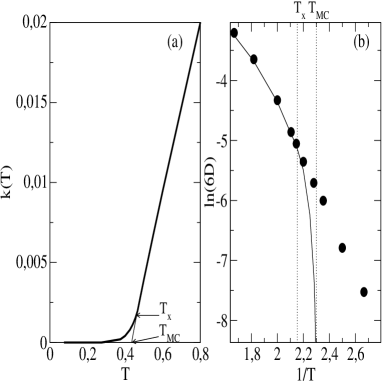
Figure 3: Figure 3(a) Density of diffusive directions $k(T)$ vs. temperature $T$ for Case (C) (thin line) and Case (D) (thick line). $T_{\mbox{\scriptsize MC}}$ marks the value $k(T)=0$ for Case (c) and $T_{\times}$ marks the change on topography of the PEL for Case (D). Figure 3(b) shows $\ln(6D)$ vs. $1/T$ for Case (D) (black points). Continuous line represents the behavior for the pure fragile glass former. $T_{\mbox{\scriptsize MC}}$ and $T_{\times}$ are marked with dotted lines.

6 Conclusions

To conclude, we have analyzed the diffusion in a supercooled liquid based solely on the density of diffusive directions and activated processes and have shown how the PEL provides an explanation for the $\beta$ and $\alpha$ relaxations and the fragility characteristics of a glassy system. The $\beta$ relaxation is directly related to the attempts of the system to move through the diffusive directions. The PEL shows that a “strong” liquid is one in which the main mechanisms of diffusion are “activated dynamics” and that a “fragile” liquid exhibits dynamics typical of supercooled liquids with diffusive directions but very high barriers where hopping is almost impossible. In this case PEL supports the same dynamical arrest behavior predicted by MCT. The crossover from fragile to strong is found to be related to a change on the topography of the PEL at a certain crossover temperature $T_{\times}$, where the density of diffusive directions changes from power-law to Arrhenius.

We would like to thank F. Sciortino and N. Giovambattista for useful discussions, and the Spanish Ministry of Education and the NSF Chemistry Program for support.

References

- [1] C.A. Angell, J. Phys. Chem. Solids 49, 863 (1988).
- [2] T. Geszti, J. Phys. C 16, 5805 (1983).
- [3] M. Goldstein , J. Chem. Phys. 51, 3728 (1969).
- [4] U. Bengtzelius, W. Götze and A. Sjölander, J. Phys. C 17 5915 (1984).
- [5] W. Götze and L. Sjögren, Rep. Prog. Phys. 55 241 (1992).
- [6] W. Götze and L. Sjögren, Transp. TheoryStat. Phys. 24 801 (1995).
- [7] W. Götze, J. Phys. Cond. Matt. 11 A1 (1999).
- [8] W. Kob, J. Phys. Cond. Matt. 11 R85 (1999).
- [9] W. Kob and H.C. Andersen, Phys. Rev. E 51 4626 (1995).
- [10] F. H. Stillinger and T. A. Weber, Science 225, 983 (1984); F. H. Stillinger, Science 267, 1935 (1995).
- [11] S. Sastry, P. G. Debenedetti and F. H. Stillinger, Nature (London) 393, 554 (1998).
- [12] S. Büchner and A. Heuer, Phys. Rev. E 60 6507 (1999).
- [13] F. Sciortino, W. Kob and P. Tartaglia, Phys. Rev. Lett. 83, 3214 (1999).
- [14] S. Sastry, Nature (London) 409, 164 (2001).
- [15] L. Angelani, G. Parisi, G. Ruocco and G. Viliani, Phys. Rev. Lett. 81 4648 (1998).
- [16] P. G, Debenedetti and F. H. Stillinger, Nature (London) 410, 259 (2001).
- [17] T. Keyes, J. Phys. Chem. 101, 2921 (1997); T. Keyes, G. V. Vijayadamodar and U. Zurcher, J. Chem. Phys. 106, 4651 (1997); W. X. Li and T. Keyes, J. Chem. Phys. 111, 5503 (1999); T. Keyes, J. Chowdahary and J. Kim, Phys. Rev. E 66, 051110 (2002).
- [18] C. Donati, F. Sciortino and P. Tartaglia, Phys. Rev. Lett. 85, 1464 (2000).
- [19] E. La Nave, A. Scala, F. W. Starr, H. E. Stanley and F. Sciortino, Phys. Rev. E 64, 036102 (2001).
- [20] S. D. Bembenek and B. B. Laird, J. Chem. Phys. 104, 5199 (1996).
- [21] L. Angelani, R. Di Leonardo, G. Ruocco, A. Scala and F. Sciortino, Phys. Rev. Lett. 85, 5356 (2000).
- [22] K. Broderix, K. K. Bhattacharya, A. Cavagna, A. Zippelius and I. Giardina, Phys. Rev. Lett. 85, 5360 (2000).
- [23] T. S. Grigera, A. Cavagna, I. Giardina and G. Parisi, Phys. Rev. Lett. 88, 055502 (2002).
- [24] L. Angelani, G. Ruocco, M. Sampoli and F. Sciortino, J. Chem. Phys. 119, 2120 (2003).
- [25] A. Gavagna, Europhys. Lett. 53, 490 (2001).
- [26] E. La Nave, H. E. Stanley and F. Sciortino, Phys. Rev. Lett. 88, 035501 (2002).
- [27] G. Fabricius and D. A. Stariolo, Phys. Rev. E 66, 031501 (2002).
- [28] M. S. Shell, P. G. Debenedetti and A. Z. Panagiotopoulos, Phys. Rev. Lett. 92, 035506 (2004).
- [29] B. Doliwa and A. Heuer, Phys. Rev. E 67, 031506 (2003).
- [30] See e.g., E. Rössler, K. -U. Hess and V. N. Novikov, J. of Non-Crystalline Solids 223, 207 (1998)