Modelling transient absorption and thermal conductivity in a simple nanofluid

Abstract

Molecular dynamics simulations are used to simulate the thermal properties of a model fluid containing nanoparticles (nanofluid). By modelling transient absorption experiments, we show that they provide a reliable determination of interfacial resistance between the particle and the fluid. The flexibility of molecular simulation allows us to consider separately the effect of confinement, particle mass and Brownian motion on the thermal transfer between fluid and particle. Finally, we show that in the absence of collective effects, the heat conductivity of the nanofluid is well described by the classical Maxwell Garnet equation model.

Many experimental studies have suggested that the thermal conductivity of colloidal suspensions referred to as “nanofluids” is unusually high Eastman ; Patel . Predictions of effective medium theories are accurate in some cases Putnam-poly but generally fail to account for the large enhancement in conductivity. In spite of a large number of - sometimes conflicting or controversial - suggestions and experimental findings Keblinski-Cahill , the microscopic mechanisms for such an increase remain unclear. Among the possibilities that were suggested, the Brownian motion prasher of a single sphere in a liquid leads to an increase in thermal conductivity of the order of $4-5\%$, and appears to be an attractive and generic explanation. The essential idea is that the Brownian velocity of the suspended particle induces a fluctuating hydrodynamic flow Alder ; Keblinski-flow , which on average influences (increases) thermal transport. This mechanism is different from transport of heat through center of mass diffusion, which was previously shown to be negligible Keblinski . However, some recent experimental high precision studies reported a normal conductivity in nanoparticle suspensions at very small volume fractions below 1% putnam , questioning the validity of this assumption.

In this work we use nonequilibrium molecular dynamics ”experiments” to explore further the transfer of heat in a model fluid containing nanoparticles. Our approach is closely related to experimental techniques, but we also make use of the flexibility allowed by molecular simulations to explore extreme cases in terms e.g. particle/fluid mass density mismatch. We concentrate on model systems that are expected to be representative of generic properties.

We start our study by mimicking the ”pump-probe” experiments that are used in nanofluids to estimate interfacial resistance, which is an essential ingredient in modelling the thermal properties of highly dispersed system pump-probe-Cahill . All atoms in our system interact through Lennard-Jones interactions

$$U_{lj}(r)=\bigg{\{}\begin{array}[]{lll}4\varepsilon((\sigma/r)^{12}-c(\sigma/r)^{6}),&r\leq r_{c}\\ 0,&r>r_{c}\end{array}$$ (1)

where $r_{c}=2.5\sigma$. The coefficient $c$ is equal to 1 for atoms belonging to the same phase, but can be adjusted to modify the wetting properties of the liquid on the solid particle barratbocquet ; barratchiaruttini . Within the solid particle, atoms are linked with their neighbors through a FENE (Finite extension non-linear elastic) bonding potential:

$$U_{FENE}(r)=\frac{k}{2}R_{0}\ln(1-(\frac{r}{R_{0}})^{2}),\qquad r<R_{0}$$ (2)

where $R_{0}=1.5\sigma$ and $k=30.0\varepsilon/\sigma^{2}$. The solid particle in the fluid was prepared as follows: starting from a FCC bulk arrangement of atoms at zero temperature, the atoms within a sphere were linked to their first neighbors by the FENE bond. Then the system was equilibrated in a constant NVE ensemble with energy value corresponding to a temperature $T=1$. The particle contains 555 atoms, surrounded by 30000 atoms of liquid. The number density in the system is $\rho=0.85\sigma^{-3}$. Taking $\sigma=0.3nm$ this corresponds to a particle radius of order $R_{part}\sim 1.5nm$ and to a system size $L\sim 10nm$.

The transient absorption simulation starts with an equilibrium configuration at temperature $T=1$, by ”heating” uniformly the nanoparticle. This heating is achieved by rescaling the velocities of all atoms within the solid particles, so that the kinetic energy per atom is equal to $3\epsilon$. We then monitor the kinetic energy per atom of the particle as a function of time, which we take as a measure of the particle temperature. The system evolves at constant energy, but the average temperature of the liquid, which acts essentially as a reservoir, is only very weekly affected by the cooling process. Within a few time steps the kinetic temperature of the particle drops to a value of $T_{p}\approx 2$. This evolution corresponds to the standard one for an isolated, harmonic system. As the particle was equilibrated at $T_{p}=1$, we have due to kinetic and potential energy equipartition $\langle E_{pot}(t=0)\rangle=1/2$. As we start our simulation with $\langle E_{k}(t=0)\rangle=3$, within a very short time the kinetic energy drops to a value of $1.5$, then the potential energy stored in the particle atoms positions yields its contribution of $1/2$ to the temperature, equilibrating it to a value of $2$. This first step does not involve any heat exchange with the liquid surroundings.

The subsequent decrease of the particle temperature, on the other hand, directly probes such exchanges. A quantitative understanding of this decay is particularly important, as it remains an essential experimental tool to quantify heat transfer across the particle-liquid interface. In figure 1, we compare the molecular dynamics simulation result for the temperature as a function of time, to the result of a continuum calculation involving the interfacial (Kapitza) thermal resistance as an adjustable parameter. The continuum calculation makes use of the standard heat transfer equations

$$C\frac{dT_{p}}{dt} = -4\pi R_{p}^{2}j(R_{p},t)$$ (3)

$$\frac{\partial T_{l}}{\partial t} = D_{th}\frac{1}{r^{2}}\frac{\partial}{\partial r}\bigg{(}r^{2}\frac{\partial T_{l}(r,t)}{\partial r}\bigg{)}$$ (4)

where $T_{l}(r,t)$ and $T_{p}$ are the liquid and particle temperatures, respectively. $C$ is the thermal capacity of the particle, $R_{p}$ its radius, $D_{th}$ is the thermal diffusion coefficient of the liquid. The above equations are solved with the following boundary conditions:

$$j(R_{p},t) = \frac{1}{R_{k}}\big{(}T_{l}(R_{p}^{+},t)-T_{p}(t)\big{)}$$ (5)

$$j(R_{\infty},t) = 0$$ (6)

where $R_{\infty}$ is chosen so that $\frac{4}{3}\pi R_{\infty}^{3}$ is equal to the volume of the simulation box from the previous section. The initial condition is

$$T_{p}(0) = 2$$ (7)

$$T_{l}(r,0) = 1$$ (8)

The temperature was assumed to be uniform inside the nanoparticle. This assumption is based on the simulation results, where the observed temperature profile inside the particle was found independent of position within statistical accuracy. We used data found in the literature barratchiaruttini ; palmer for the values of the fluid thermal diffusivity and conductivity. As the simulated particle is not exactly spherical, but presents some FCC facets, its radius for use in the calculation was estimated from the radius of gyration:

$$\langle R_{g}^{2}\rangle=\frac{1}{N}\sum_{1}^{N}(r_{i}-r_{CM})^{2}=\frac{3}{5}R_{p}^{2}$$ (9)

where $R_{g}^{2}$ is the measured radius of gyration of the particle atoms, and the second equality applies to an ideal sphere. In the range $T=1$ to $T=3.5$, we checked through equilibrium simulations that the heat capacity of the particle is very close to $3k_{B}TN$, as for an harmonic ideal solid.

The value of the interface thermal resistance (Kapitza resistance) appearing in equation 6 was adjusted to fit the simulation data. The value that fits the simulation results for the wetting system $m=1$ and $c=1$ was found to be $R_{K}\approx 0.8$. This number is in agreement with the thermal resistance for a wetting flat wall calculated in barratchiaruttini for a similar system with a different potential in the solid phase, and a completely different simulation method.

The same cooling simulation was performed using a non wetting particle ($c=0.5$). A substantial slowing down of the cooling rate was also observed, which can be attributed to an increased Kapitza resistance. The resulting value of $R_{K}$ is 3.2 (Lennard-Jones unit), again in agreement with previous determinations for flat surfaces barratchiaruttini . In real units, a value $R_{K}=1$ corresponds typically to an interfacial conductance $G=1/R_{K}$, of the order of $100\mathrm{MW/Km}^{2}$ . The method is therefore a sensitive probe of interfacial resistance, as usually assumed in experiments.

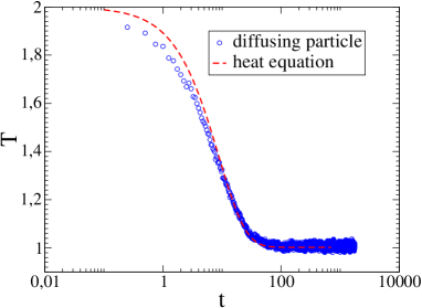
Figure 1: Comparison between the temperature evolution from simulations and the solution of the continuum heat equation. The value of the Kapitza resistance taken for the calculation is $R_{K}=0.8$.

In a second step, we explore the influence of thermal Brownian motion of the particle on the cooling process. First, let us recall that the naive idea, that diffusion could speed up cooling by displacing the particles towards cooler fluid regions is easily excluded. Quantitatively, diffusion of the particle and heat diffusion take place on very different time scales. The diffusion coefficient of the particle was measured, in our case, to be three orders of magnitude smaller than the heat diffusion coefficient in the fluid. We also suppressed diffusion by tethering the particle to its initial position with a harmonic spring of stiffness $k=30\epsilon/\sigma^{2}$. As expected, no effect is observable on the cooling rate. This measurement cannot probe for another possible effect - the influence of fluid flow on the cooling. As discussed in Acrivos the heat transfer from a sphere in a low Reynolds number velocity field is enhanced by the latter. Because of the diffusion velocity of the Brownian particle $v=\big{(}\frac{3k_{B}T}{m}\big{)}^{1/2}$, it can be viewed, at any given moment, as a particle in a velocity field prasher . To probe the influence of this phenomenon, we tether every single atom in the particle to its initial position with a harmonic spring ($k=30$) and compare the measured temperature evolution with the previous results. The cooling rate is still not influenced by this manipulation even if the center of mass is now “frozen” (fig. 2).

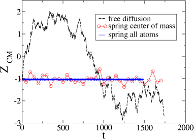
Figure 2: Evolution of the $Z$ coordinate of the particle center of mass for the different systems: free particle, particle confined by a spring attached to its center of mass and particle where all atoms are tethered to their initial position. The spring constant for all springs is $k=30$.

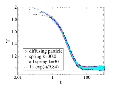
Figure 3: The evolution of the particle temperature for the different systems: free particle, particle confined by a spring attached to its center of mass and particle where all atoms are tethered to their initial position. Every curve is the mean value from 20 simulation runs. No effect is observed.

A final check on the influence of such velocity effects was attempted by modifying the mass of the atoms that constitute the nanoparticle. This artificial procedure reduces the thermal Brownian velocity, and when it is carried out we indeed observe a strong slowing down of the cooling process. However, this slowing down is again completely independent of the center of mass motion of the particle, which is controlled by the presence of the tethering springs. On the other hand, the effect of this mass density increase is easily understood in terms of an increase of the interfacial resistance. A higher mass of the particle atoms decreases the speed of sound in the solid and thus leads to a larger acoustic mismatch between the two media, which slows down the cooling. Numerically, we find that for a mass of $100$ times the mass of a liquid atom, the Kapitza resistance increases to $R_{K}=7.4$.

In summary, we have shown that the Brownian motion of the particle does not affect the cooling process. As a byproduct, we have shown that the mass density parameter provides a flexible numerical way of tuning the interfacial resistance, which will be used in the next section.

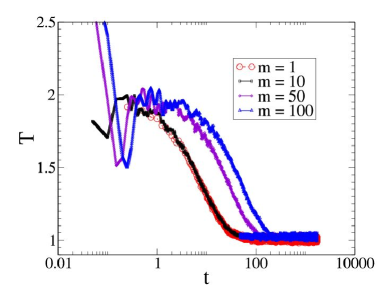
Figure 4: The evolution of the particle temperature as a function of the mass of the particle atoms. Every curve is the mean value from 20 simulation runs. The increased mass slows down heat exchange.

In this last section, we attempt direct measurements of the nanofluid heat conductivity using a nonequilibrium molecular dynamics simulation of heat transfer across a fluid slab containing one nanoparticle, with periodic boundary conditions in the $x$ and $y$ direction and confined by a flat repulsive potential in the $z$ direction.

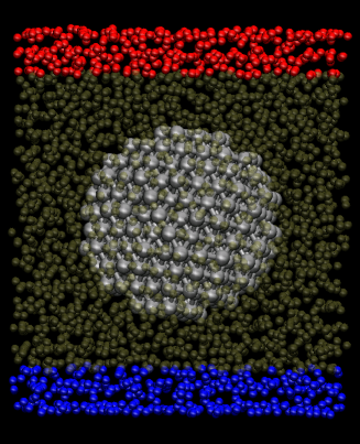
Figure 5: Snapshot of the system used to evaluate the thermal conductivity with a particle of 13% volume fraction.

Two slices of fluid are thermostated, using velocity rescaling, at different temperatures. To avoid any effect of thermophoresis or coupling of the thermostat the particle, the particle is constrained to stay at equal distance between the two thermostats using two different schemes. First, a confinement between two repulsive, parallel walls, that couple only to the particle atoms. The particle is then constrained to the mid-plane of the simulation cell, but free to diffuse within this plane. The second possibility is to tether the center of mass to a fixed point, as described above, so that any possible effect due to flow or diffusion is eliminated. The energy flux is measured by calculating the energy absorbed by the thermostats. The effective conductivity of the system was defined as:

$$\lambda_{eff}=\frac{J}{(T_{1}-T_{2})/L}$$ (10)

The temperatures of the two thermostats were $T_{1}=2$ and $T_{2}=1$. In order to compare the conductivity results for the different systems they were first equilibrated to the same pressure at a temperature $T=1.5$, then a non equilibrium run was performed for about 1500-2000 $\tau_{LJ}$ to make sure the pressure stays the same for the systems of different nature and finally a production run of about 30000 $\tau_{LJ}$ during which thermostats energy, particle diffusion and temperature profiles are monitored. Simulations were performed with two different volume fractions for the particle, 2% or 13%. The volume fraction is defined as the volume of the particle divided by the volume of the fluid outside the thermostats. As expected from the study above, no effect of the particle diffusion on the fluid conductivity was observed. The effective conductivity measured for the particle diffusing in 2D, the particle attached with a single spring or the particle where all atoms were attached to their initial positions has the same value within 1% which is below the error bar of the measurement (around 4-5%). Finally, we investigated the effect of the presence of the nanoparticle on the thermal conductivity of the fluid. For the smallest volume fraction ($\Phi\sim 2\%$), we were not able to detect any change in thermal conductivity compared to the bulk fluid. At the higher volume fraction ($\Phi\sim 13\%$), on the other hand, we observe a clear decrease in the heat conductivity associated with the presence of the nanoparticle (fig. 6). Clearly, this decrease must be interpreted in terms of interfacial effects. To quantify these effects, we use the Maxwell-Garnett approximation for spherical particles, modified to account account for the Kapitza resistance at the boundary between the two media. The resulting expression for the effective conductivity MG is

$$\frac{\lambda_{eff}}{\lambda_{l}}=\frac{\big{(}\frac{\lambda_{p}}{\lambda_{l}}(1+2\alpha)+2\big{)}+2\Phi\big{(}\frac{\lambda_{p}}{\lambda_{l}}(1-\alpha)-1\big{)}}{\big{(}\frac{\lambda_{p}}{\lambda_{l}}(1+2\alpha)+2\big{)}-\Phi\big{(}\frac{\lambda_{p}}{\lambda_{l}}(1-\alpha)-1\big{)}}$$ (11)

where $\lambda_{l}$ and $\lambda_{p}$ are the liquid and particle conductivities, $\Phi$ is the particle volume fraction and $\alpha=\frac{R_{K}\lambda_{l}}{R_{p}}$ is the ratio between the Kapitza length (equivalent thermal thickness of the interface) and the particle radius. This model predicts an increase in the effective conductivity for $\alpha>1$ and a decrease for $\alpha<1$, regardless of the value of the conductivity of the particles or of the volume fraction. The prediction depends very weekly on the ratio $\lambda_{p}/\lambda_{l}$, less than 1% for $10<\lambda_{p}/\lambda_{l}<100$. The minimum value of $\lambda_{eff}/\lambda_{l}$, obtained when $\alpha\to\infty$, is $\frac{1-\Phi}{1+\Phi/2}$ while the maximum possible enhancement (for $\lambda_{p}\to\infty$ and $R_{K}\to 0$) is $\frac{1+2\Phi}{1-\Phi}$.

As explained above, the Kapitza resistance can be modified by tuning either the liquid solid interaction coefficient $c$, or the mass density of the solid, or a combination thereof. Figure 6 illustrates the variation of the measured effective conductivity for several values of the Kapitza resistance, determined independently for various values of these parameters. It is seen that the observed variation (decrease in our case) in the effective conductivity is very well described by the Maxwell-Garnett expression. This expression also allows us to understand why the heat conductivity does not vary in a perceptible manner for the smaller volume fraction, for which the predicted change would be less than $3\%$, within our statistical accuracy.

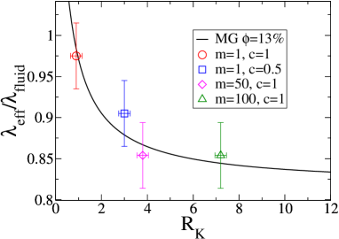
Figure 6: Comparison between the ratio of the effective conductivity to the conductivity of the pure liquid of the simulated systems and the values obtained from the Maxwell Garnett equation. The values of the Kapitza resistance for the simulations were obtained from the cooling rate of the particle.

Conclusion

We have explored some important aspects of the thermal properties of ”nanofluids”, at the level of model system and individual solid particles. The molecular modeling of transient heating experiments confirms that they are a sensitive tool for the determination of thermal boundary resistances. The effect of Brownian motion on the cooling process, on the other hand, was found to be negligible. By varying interaction parameters or mass density, we are able to vary the interfacial resistance between the particle and the fluid in a large range. This allowed us to estimate, over a large range of parameters, the effective heat conductivity of a model nanofluid in which the particles would be perfectly dispersed. Our results can be simply explained in terms of the classical Maxwell-Garnett model, provided the interfacial resistance is taken into account. The essential parameter that influences the effective conductivity turns out to be the ratio between the Kapitza length and the particle radius, and for very small particles a decrease in conductivity compared to bulk fluids is found. We conclude that large heat transfer enhancements observed in nanofluids must originate from collective effects, possibly involving particle clustering and percolation or cooperative heat transfer modes.

References

- [1] Eastman, J. A.; Choi, S. U. S.; Li, S.; Yu, W.; Thompson, L. J.; Appl. Phys. Lett. 2001, 78, 718.
- [2] Patel, H. E.; Das, S. K.; Sundararajan T.; Nair, A. S.; George, B.; Pradeep, T.; Appl. Phys. Lett. 2003, 83, 2931.
- [3] Putnam, S. A.; Cahill, D. A.; Ash, B. J.; Schadler, L. S.; J. Appl. Phys., 2003, 94, 6785.
- [4] Keblinski, P.; Eastman, J. A.; Cahill, D. A.; Materials Today, 2005, 8, 36.
- [5] Prasher, R.; Bhattacharya, P.; Phelan, P. E.; Phys. Rev. Lett. 2005, 94, 025901.
- [6] Alder, B.J.; Wainwright, T.E.; Phys. Rev. A, 1970, 1, 18.
- [7] Keblinski, P.; Thomin, J.; Phys. Rev. E 73, 010502 (2006)
- [8] Keblinski, P.; Phillot, S. R.; Choi, S. U.-S.; Eastman, J. A.; Int. J. of Heat and Mass Transf. 2002, 45, 855.
- [9] Putnam, S. A.; Cahill, D. G.; P. V. Braun, P. V.; Ge, Z.; Shimmin R. G.; J. Appl. Phys., in press
- [10] Wilson, O. M.; Hu, X.; Cahill, D. G.; Braun, P. V.; Phys. Rev. B 2002, 66, 224301.
- [11] Barrat, J.-L.; Bocquet, L.; Faraday Discussions 1999, 112, 121.
- [12] Barrat, J.-L.; Chiaruttini, F.; Molecular Physics 2003, 101, 1605.
- [13] Acrivos, A.; Taylor, T. D.; Physics of Fluids 1962, 5, 387.
- [14] Palmer, B. J.; Phys. Rev. E 1994, 49, 2049.
- [15] Nan, C. W.; Birringer, R.; Clarke, D. R.; Gleiter, H.; J. Appl. Phys., 1997, 81, 6692.