Dynamic structure factor of the Calogero-Sutherland model

Michael Pustilnik School of Physics, Georgia Institute of Technology, Atlanta, GA 30332
Abstract

We evaluate the dynamic structure factor $S(q,\omega)$ of a one-dimensional quantum Hamiltonian with the inverse-square interaction (Calogero-Sutherland model). For a fixed small $q$, the structure factor differs from zero in a finite interval of frequencies of the width $\delta\omega\propto q^{2}\!/m$. At the borders of this interval $S(q,\omega)$ exhibits power-law singularities with exponents depending on the interaction strength. The singularities are similar in origin to the well-known Fermi-edge singularity in the x-ray absorption spectra of metals.

pacs:
71.10.Pm, 02.30.Ik, 72.15.Nj

Fermi liquid theory proved to be extremely successful in describing interacting fermionsΒ Nozieres . The low-energy excitations of a normal Fermi liquid (FL) are classified the same way as the excitations of a reference system - a non-interacting Fermi gas. A weak residual interaction leads to a finite decay rate $1\!/\tau$ of FL’s quasiparticles. Formally, the rate can be defined as the width of the quasiparticle peak in the spectral function (imaginary part of a single-particle retarded Green function) $A(q,\omega)$. For FL, $A(q,\omega)$ at $T=0$ is a Lorentzian. Its width is easily evaluated in the second order of perturbation theory, which yields $1\!/\tau\propto\omega^{2}\!/\epsilon_{F}$, where $\omega(q)$ is the quasiparticle energy.

It is well-known, however, that in one dimension (1D) even a weak interaction breaks down the FL description (seeΒ 1D_books for recent reviews). A guide to understanding the properties of interacting 1D systems is provided by the Tomonaga-Luttinger model (TLM)Β TL , which plays the same role for the concept of the Luttinger liquidΒ Haldane as the Fermi gas does for FL. The TLM assumes a strictly linear fermionic dispersion relation. With this assumption, the TLM Hamiltonian can be diagonalized exactlyΒ TL , no matter how strong the interactions are. The corresponding elementary excitations are bosons, quanta of the waves of fermionic density. These bosons do not interact, have an infinite lifetime, and propagate without dispersion, $\omega(q)=uq$ (here $u$ is the plasma velocity). Therefore, a measurable quantity, the dynamic structure factor (density-density correlation function)Β structure_factor

$$S(q,\omega)=\int\!dx\,dt\,e^{i(\omega t-qx)}\bigl{\langle}\rho(x,t)\rho(0,0)\bigr{\rangle},$$ (1)

has an infinitely sharp peak, $S_{\text{TLM}}(q,\omega)\propto q\delta(\omega-uq)$.

Applications of TLM to the description of β€œreal” 1D fermions rely on the expansion of single-particle energies about the Fermi points $\pm\,p_{F}$Β 1D_books ; Haldane ,

$$\xi_{k}=\pm\,v_{F}k+k^{2}\!/2m+\ldots,\quad k=p\mp p_{F},$$ (2)

where the upper/lower sign corresponds to the right/left movers (throughout this Letter we use units with $\hbar=1$). The linear in $k$ term in Eq.Β (2) is accounted for in TLM. The $k^{2}$ term generates interaction between the bosons with the coupling constant $\propto 1\!/m$Β Haldane , which broadens the peak in $S(q,\omega)$. However, in contrast with FL theory, this broadening is inaccessible by perturbation theory.

This can be seen by considering a special limit of LL, that of non-interacting fermions with spectrum (2). In this case the structure factor differs from zero only if $\omega$ lies within a finite interval $\omega_{-}<\omega<\omega_{+},$ where $\omega_{\pm}(q)=v_{F}q\pm\,q^{2}\!/2m$ for $q<2p_{F}$. Within this interval $S(q,\omega)$ is constant, $S=m/q$. Thus, at $q\to 0$ the structure factor indeed approaches the TLM form (with $u=v_{F}$), but in a very peculiar fashion: the peak in $S(q,\omega)$ at a fixed $q$ has a manifestly non-Lorentzian β€œrectangular” shape with the width $\delta\omega=q^{2}\!/m$. Even this simple result is non-perturbative in the bosonic representation: the first-order in $1/m$ contribution to the boson’s self-energy vanishes, while the next one diverges on the mass shellΒ Samokhin .

Recently it was argued Β 1DEG that in the presence of interactions between the fermions the shape of the peak in $S(q,\omega)$ remains to be non-Lorentzian. Moreover, even a weak interaction transforms the discontinuities at $\omega=\omega_{\pm}$ into power-law singularities. Here we approach the problem of finding $S(q,\omega)$ from the perspective of the exactly solvable Calogero-Sutherland model (CSM).

The CSM Hamiltonian readsΒ Sutherland

$$H=-\sum_{i=1}^{N}\frac{1}{2m}\frac{\partial^{2}}{\partial x_{i}^{2}}+\sum_{i<j}V(x_{i}-x_{j}),$$ (3)

where $V(x)$ is a periodic version of $1/x^{2}$ potential,

$$V(x)=\frac{\lambda(\lambda-1)\!/m}{(L/\pi)^{2}\sin^{2}\!\bigl{(}\pi x/L\bigr{)}}\,.$$ (4)

The excitations of CSM can be described in terms of quasiparticles and quasiholesΒ Sutherland . Quasiparticles are characterized by velocities $v$ in the range $|v|>u$, and an inertial mass $m$, the bare mass that enters Eq.Β (3). Quasiholes have velocities $\bar{v}$ in the range $|\bar{v}|<u$, and fractional inertial mass $\bar{m}=m/\lambda$. The plasma velocity $u$ is given byΒ Sutherland

$$u=\pi\lambda\rho_{0}/m,\quad\rho_{0}=N/L.$$ (5)

The momentum and energy (relative to the ground state) of an excited state of CSM characterized by a certain set of velocities $\{v_{i},\bar{v}_{j}\}$ read Sutherland

$\displaystyle P$ $\displaystyle=$ $\displaystyle\sum_{i}mv_{i}-\sum_{j}\bar{m}\bar{v}_{j}$ (6)
$\displaystyle E$ $\displaystyle=$ $\displaystyle\sum_{i}\frac{1}{2}\,m\bigl{(}v_{i}^{2}-u^{2}\bigr{)}+\sum_{j}\frac{1}{2}\,\bar{m}\bigl{(}u^{2}-\bar{v}_{j}^{2}\bigr{)}.$ (7)

The result of the action of the local density operator

ρq†=∫0L𝑑x​ei​q​x​ρ​(x),ρ​(x)=1Lβ€‹βˆ‘i=1Nδ​(xβˆ’xi)βˆ’Ο0formulae-sequencesubscriptsuperscriptπœŒβ€ π‘žsuperscriptsubscript0𝐿differential-dπ‘₯superscriptπ‘’π‘–π‘žπ‘₯𝜌π‘₯𝜌π‘₯1𝐿superscriptsubscript𝑖1𝑁𝛿π‘₯subscriptπ‘₯𝑖subscript𝜌0\rho^{\dagger}_{q}=\int_{0}^{L}\!dx\,e^{iqx}\rho(x),\quad\rho(x)=\frac{1}{L}\sum_{i=1}^{N}\delta(x-x_{i})-\rho_{0}

on CSM’s ground state |0⟩delimited-|⟩0\left\lvert{0}\right\rangle has a remarkable propertyΒ Ha : ρq†|0⟩\rho^{\dagger}_{q}\left\lvert{0}\right\rangle is an eigenstate of CSM in which the velocities of all quasiparticles point in the same direction (positive for q>0π‘ž0q>0). This has a profound effect on the structure factor: S​(q,Ο‰)β‰ 0π‘†π‘žπœ”0S(q,\omega)\neq 0 
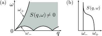
only in a finite interval of frequencies, Ο‰βˆ’β€‹(q)<Ο‰<Ο‰+​(q)subscriptπœ”π‘žπœ”subscriptπœ”π‘ž\omega_{-}(q)<\omega<\omega_{+}(q), see Fig.Β 1(a) (the upper bound Ο‰+subscriptπœ”\omega_{+} would be absent in a generic 1D systemΒ 1DEG ).

Refer to caption
Figure 1: (a) The structure factor $S(q,\omega)$ differs from zero in a finite interval of frequencies $\omega_{-}\!\!<\!\omega\!<\!\omega_{+}$. At the borders of this interval $S(q,\omega)$ exhibits power-law singularities, $S\propto|\omega-\omega_{\pm}|^{\lambda^{\pm 1}-1}$, see Eqs. (21) and (22). The low-energy $(\omega_{-}\to 0)$ sectors correspond to $q=2\pi\rho_{0}I$, where $I$ is an integer. (b) Dependence of $S(q,\omega)$ on $\omega$ at a fixed qβ‰ 2​π​ρ0​Iπ‘ž2πœ‹subscript𝜌0𝐼q\neq 2\pi\rho_{0}I and for a repulsive interaction $(\lambda>1)$.

From this point on, we consider the rational values of $\lambda$ only, Ξ»=r/sπœ†π‘Ÿπ‘ \lambda=r/s, where $r$ and $s$ are co-primes. In this case, the state $\left\lvert{R}\right\rangle=\rho^{\dagger}_{q>0}\left\lvert{0}\right\rangle$ has exactly $s$ right-moving quasiparticles and exactly $r$ quasiholes Haldane_conjecture ; ZH ; Ha . This is the simplest possible excitation that conserves the total inertial mass,

s​mβˆ’r​mΒ―=0​for​λ=r/s.π‘ π‘šπ‘ŸΒ―π‘š0forπœ†π‘Ÿπ‘ sm-r\bar{m}=0~{}~{}\text{for}~{}~{}\lambda=r/s. (8)

The bounds $\omega_{\pm}$ are easily found from the momentum and energy conservation,

$$q=P_{\,\left\lvert{R}\right\rangle},\quad\omega=E_{\left\lvert{R}\right\rangle}.$$ (9)

Indeed, it follows from Eqs. (6)-(9) that

$\displaystyle q\!$ $\displaystyle=$ βˆ‘i=1sm​(viβˆ’u)+βˆ‘j=1rm¯​(uβˆ’vΒ―j),superscriptsubscript𝑖1π‘ π‘šsubscript𝑣𝑖𝑒superscriptsubscript𝑗1π‘ŸΒ―π‘šπ‘’subscript¯𝑣𝑗\displaystyle\!\sum_{i=1}^{s}m(v_{i}-u)+\,\sum_{j=1}^{r}\bar{m}(u-\bar{v}_{j}), (10)
$\displaystyle 2(\omega-uq)\!$ $\displaystyle=$ βˆ‘i=1sm​(viβˆ’u)2βˆ’βˆ‘j=1rm¯​(uβˆ’vΒ―j)2.superscriptsubscript𝑖1π‘ π‘šsuperscriptsubscript𝑣𝑖𝑒2superscriptsubscript𝑗1π‘ŸΒ―π‘šsuperscript𝑒subscript¯𝑣𝑗2\displaystyle\!\sum_{i=1}^{s}m(v_{i}-u)^{2}-\,\sum_{j=1}^{r}\bar{m}(u-\bar{v}_{j})^{2}.\qquad (11)

Since $v_{i}-u\geq 0$ and $u-\bar{v}_{j}\geq 0$, Eq.Β (10) implies that for a given $q<2\pi\rho_{0}$ the velocities vary in the range

$$\begin{array}[]{cl}\,u<v_{i}<v_{0},&\quad v_{0}=u+q/m,\\ \bar{v}_{0}\!<\bar{v}_{j}\!<u,&\quad\bar{v}_{0}=u-q/\bar{m}.\end{array}$$ (12)

The upper bound $\omega=\omega_{+}$ is reached when the velocity of one of the quasiparticles approaches $v_{0}$ while all the remaining quasiparticles/holes have velocities close to the plasma velocity $u$. Eq.Β (11) then gives

$$\omega_{+}-uq=\frac{m}{2}\,(v_{0}-u)^{2}=\frac{\,q^{2}}{2m}.$$ (13)

Similarly, the lower bound $\omega_{-}$ corresponds to the intermediate state $\left\lvert{R}\right\rangle$ in which one of the quasiholes has velocity close to $\bar{v}_{0}$, while the velocities of all the remaining quasiparticles/holes are close to $u$, so that

$$\omega_{-}-uq=-\frac{\bar{m}}{2}\,(u-\bar{v}_{0})^{2}=-\frac{\,q^{2}}{2\bar{m}}=-\lambda\frac{\,q^{2}}{2m}\,.$$ (14)

The width of the region where Sβ‰ 0𝑆0S\neq 0 is then given byΒ drag

$$\delta\omega=\omega_{+}-\omega_{-}=(\lambda+1)\frac{\,q^{2}}{2m}.$$ (15)

Eq.Β (14) is valid as long as $\omega_{-}\geq 0$, i.e. for $q\leq 2\pi\rho_{0}$. At larger $q$ the function $\omega_{-}(q)$ is given by Eq.Β (14) with the replacement $q\to q-2\pi\rho_{0}I$, where $I$ is the integer part of $q/2\pi\rho_{0}$. The corresponding intermediate state $\left\lvert{R}\right\rangle$ has $I$ quasiholes with velocities approaching $-u$, one quasihole with velocity near $\bar{v}_{0}$ (given by Eq.Β (12) with the replacement $q\to q-2\pi\rho_{0}I$), and all the remaining quasiparticles/holes moving with the plasma velocity $u$.

We turn now to the evaluation of the structure factor. In the thermodynamic limit ($N\to\infty$, $\rho_{0}=\text{const}$) Eq.Β (1) can be rewritten as

S​(q,Ο‰)=q2β€‹βˆ«βˆi,jd​vi​d​vΒ―j​Fs,r​δ​(qβˆ’P|R⟩)​δ​(Ο‰βˆ’E|R⟩).π‘†π‘žπœ”superscriptπ‘ž2subscriptproduct𝑖𝑗𝑑subscript𝑣𝑖𝑑subscript¯𝑣𝑗subscriptπΉπ‘ π‘Ÿπ›Ώπ‘žsubscript𝑃delimited-|βŸ©π‘…π›Ώπœ”subscript𝐸delimited-|βŸ©π‘…S(q,\omega)=q^{2}\!\!\!\int\!\prod_{i,j}dv_{i}d\bar{v}_{j}\,F_{s,r}\,\delta\bigl{(}q-P_{\left\lvert{R}\right\rangle}\bigr{)}\,\delta\bigl{(}\omega-E_{\left\lvert{R}\right\rangle}\bigr{)}. (16)

The form-factor Fs,rsubscriptπΉπ‘ π‘ŸF_{s,r} here is given by

$$F_{s,r}\propto\frac{\prod_{i<i^{\prime}}|v_{i}-v_{i^{\prime}}|^{2\lambda}\!\prod_{j<j^{\prime}}|\bar{v}_{j}-\bar{v}_{j^{\prime}}|^{2/\lambda}}{\prod_{i,j}(v_{i}-\bar{v}_{j})^{2}\prod_{i}\,\bigl{(}v_{i}^{2}-u^{2}\bigl{)}^{1-\lambda}\prod_{j}\,\bigl{(}u^{2}-\bar{v}_{j}^{2}\bigl{)}^{1-1/\lambda}}\,.$$ (17)

(note that ∏d​vi​d​vΒ―j​Fs,rproduct𝑑subscript𝑣𝑖𝑑subscript¯𝑣𝑗subscriptπΉπ‘ π‘Ÿ\prod dv_{i}d\bar{v}_{j}F_{s,r} is dimensionless). This expression was conjectured in Haldane_conjecture based on the results of Ref.Β Altshuler for $\lambda=1/2,2$Β RMT ; the conjecture was proved in Ha using properties of Jack polynomials. In writing (17), we omitted $\lambda$-dependent numerical coefficientΒ Ha .

For simplicity, we concentrate on the most interesting limit of small $q\ll\pi\rho_{0}$. In this limit $v_{0}-u,u-\bar{v}_{0}\ll u$, see Eq.Β (12), and one can approximate $v_{i}^{2}-u^{2}\approx 2u(v_{i}-u)$, $u^{2}-\bar{v}_{j}^{2}\approx 2u(u-\bar{v}_{j})$ in Eq.Β (17). In view of the restriction (12) on the velocities, it is convenient to switch in Eq.Β (16) to the new integration variables

$$x_{i}=\frac{v_{i}-u}{v_{0}-u}\,,\quad\bar{x}_{j}=\frac{u-\bar{v}_{j}}{u-\bar{v}_{0}}\,,$$ (18)

which vary between 00 and $1$. In terms of these variables

$\displaystyle\frac{S(q,\omega)}{S_{0}(q)}\!$ $\displaystyle=$ ∫01∏d​xi​d​xΒ―j​Fs,r​δ​(βˆ‘β‘xi+βˆ‘β‘xΒ―jβˆ’1)superscriptsubscript01product𝑑subscriptπ‘₯𝑖𝑑subscriptΒ―π‘₯𝑗subscriptπΉπ‘ π‘Ÿπ›Ώsubscriptπ‘₯𝑖subscriptΒ―π‘₯𝑗1\displaystyle\!\!\int_{0}^{1}\prod dx_{i}d\bar{x}_{j}\,F_{s,r}\,\delta\Bigl{(}\operatorname{\textstyle\sum}x_{i}+\operatorname{\textstyle\sum}\bar{x}_{j}-1\Bigr{)}\qquad
$\displaystyle\qquad\times\,\delta\biggl{(}\!\operatorname{\textstyle\sum}x_{i}^{2}-\lambda\!\operatorname{\textstyle\sum}\bar{x}_{j}^{2}-(\lambda+1)\frac{\omega-uq}{\delta\omega}\biggr{)},$

where $S_{0}(q)=m/q$ is the structure factor for noninteracting fermions $(\lambda=1)$, and the form-factor is

Fs,r∝∏i<iβ€²|xiβˆ’xiβ€²|2β€‹Ξ»β€‹βˆj<jβ€²|xΒ―jβˆ’xΒ―jβ€²|2/λ∏i,j(xi+λ​xΒ―j)2β€‹βˆixi1βˆ’Ξ»β€‹βˆjxΒ―j1βˆ’1/Ξ».proportional-tosubscriptπΉπ‘ π‘Ÿsubscriptproduct𝑖superscript𝑖′superscriptsubscriptπ‘₯𝑖subscriptπ‘₯superscript𝑖′2πœ†subscriptproduct𝑗superscript𝑗′superscriptsubscriptΒ―π‘₯𝑗subscriptΒ―π‘₯superscript𝑗′2πœ†subscriptproduct𝑖𝑗superscriptsubscriptπ‘₯π‘–πœ†subscriptΒ―π‘₯𝑗2subscriptproduct𝑖superscriptsubscriptπ‘₯𝑖1πœ†subscriptproduct𝑗superscriptsubscriptΒ―π‘₯𝑗11πœ†F_{s,r}\propto\frac{\prod_{i<i^{\prime}}|x_{i}-x_{i^{\prime}}|^{2\lambda}\!\prod_{j<j^{\prime}}|\bar{x}_{j}-\bar{x}_{j^{\prime}}|^{2/\lambda}}{\prod_{i,j}(x_{i}+\lambda\bar{x}_{j})^{2}\prod_{i}x_{i}^{1-\lambda}\prod_{j}\bar{x}_{j}^{1-1/\lambda}}\,. (20)

Evaluation of Eq.Β (Dynamic structure factor of the Calogero-Sutherland model) simplifies considerably when $\omega\to\omega_{\pm}$. Consider, for example, the limit $\omega-\omega_{-}\ll\delta\omega$. In this limit the non-vanishing contributions to the integral in (Dynamic structure factor of the Calogero-Sutherland model) come from $r$ sectors of the (r+s)π‘Ÿπ‘ (r+s)-dimensional integration space in which one of $\bar{x}_{j}$, say $\bar{x}_{k}$, is close to $1$, while all the other variables approach 00. To lowest order in xi,xΒ―jβ‰ k,1βˆ’xΒ―kβ‰ͺ1much-less-thansubscriptπ‘₯𝑖subscriptΒ―π‘₯π‘—π‘˜1subscriptΒ―π‘₯π‘˜1x_{i},\bar{x}_{j\neq k},1-\bar{x}_{k}\ll 1, the second $\delta$-function in Eq.Β (Dynamic structure factor of the Calogero-Sutherland model) can be replaced by

$$\delta(\ldots)\approx\,\delta\Bigl{(}2\lambda(1-\bar{x}_{k})-(\lambda+1)\frac{\,\omega-\omega_{-}}{\delta\omega\,\,}\Bigr{)},$$

and the form-factor Fs,rsubscriptπΉπ‘ π‘ŸF_{s,r} becomes

Fs,r​({xi},{xΒ―j})β‰ˆΞ»βˆ’2​s​Fs,rβˆ’1​({xi},{xΒ―j}jβ‰ k)subscriptπΉπ‘ π‘Ÿsubscriptπ‘₯𝑖subscriptΒ―π‘₯𝑗superscriptπœ†2𝑠subscriptπΉπ‘ π‘Ÿ1subscriptπ‘₯𝑖subscriptsubscriptΒ―π‘₯π‘—π‘—π‘˜F_{s,r}\Bigl{(}\{x_{i}\},\!\{\bar{x}_{j}\}\Bigr{)}\approx\lambda^{-2s}F_{s,r-1}\Bigl{(}\{x_{i}\},\!\{\bar{x}_{j}\}_{\!j\neq k}\Bigr{)}

(Fs,rβˆ’1subscriptπΉπ‘ π‘Ÿ1F_{s,r-1} is given by (20) with $j=k$ excluded). With these approximations, the integrations in (Dynamic structure factor of the Calogero-Sutherland model) are easily carried out and yield

$$\frac{S(q,\omega)}{S_{0}(q)}\propto\left[\frac{\,\omega-\omega_{-}}{\delta\omega~{}}\right]^{1/\lambda-1},\quad 0<\omega-\omega_{-}\ll\delta\omega.$$ (21)

Similarly, at $\omega_{+}-\omega\ll\delta\omega$, the non-vanishing contributions to the integral in Eq.Β (Dynamic structure factor of the Calogero-Sutherland model) come from $s$ sectors where 1βˆ’xk,xiβ‰ k,xΒ―jβ‰ͺ1much-less-than1subscriptπ‘₯π‘˜subscriptπ‘₯π‘–π‘˜subscriptΒ―π‘₯𝑗11-x_{k},x_{i\neq k},\bar{x}_{j}\ll 1, and one finds

$$\frac{S(q,\omega)}{S_{0}(q)}\propto\left[\frac{\omega_{+}\!-\omega}{\delta\omega}\right]^{\lambda-1},\quad 0<\omega_{+}-\omega\ll\delta\omega.$$ (22)

It should be emphasized that Eqs. (21) and (22) with $q$-independent exponents are valid for all qβ‰ 2​π​ρ0​Iπ‘ž2πœ‹subscript𝜌0𝐼q\neq 2\pi\rho_{0}I, including $q\gtrsim\pi\rho_{0}$. In addition to $\omega_{\pm}(q)$, a smooth dependence on $q$ enters Eqs. (21) and (22) via the (omitted) prefactors; these $\omega$-independent prefactors tend to $1$ in the limit $\lambda\to 1$. According to Eqs. (21) and (22), the structure factor diverges at $\omega\to\omega_{-}\,(\omega_{+})$ for a repulsive (attractive) interaction, see Fig.Β 1(b); the divergencies are integrable for all physically meaningful (i.e. positive) values of $\lambda$Β square-root . Note that, formally, Eq.Β (22) can be obtained by replacing $|\omega-\omega_{-}|\to|\omega-\omega_{+}|$ and $\lambda\to 1/\lambda$ in Eq.Β (21). This correspondence is a manifestation of the particle$\,\leftrightarrow\,$hole, $\lambda\!\leftrightarrow\!1/\lambda$ duality of CSMΒ Polychronakos .

The power-law singularities in Eqs. (21) and (22) are similar to the familiar edge singularities in the x-ray absorption spectra in metalsΒ Mahan . Consider, for example, the limit $\omega\to\omega_{+}$. In this case the action of the operator ρq†superscriptsubscriptπœŒπ‘žβ€ \rho_{q}^{\dagger} on the ground state creates a quasiparticle at $k\approx q$ with energy $\approx\omega_{+}$. This high-energy quasiparticle interacts with the Fermi sea, resulting in the excitation of multiple low-energy particle-hole pairs, just like the core hole does in the conventional x-ray edge singularity. The proliferation of the low-energy particle-hole pairs leads to the singularity in the response functionΒ 1DEG ; Furusaki .

This analogy suggests that, just like in the case of the conventional edge singularity, the functional form of the dependence of the structure factor on $\omega-\omega_{+}$ can be captured by replacing the original model with the properly chosen effective Hamiltonian. For $\omega\to\omega_{+}$ and $q\ll\pi\rho_{0}$ it is sufficient to include in the effective Hamiltonian only the right-moving single-particle states within two very narrow stripes (subbands) of momenta near $k=q$ and $k=0$Β 1DEG to allow for both the creation of the high-energy quasiparticle and the low-energy particle-hole pairs. (Recall that for $q\!<\!\pi\rho_{0}$ the velocities of all quasiparticles/holes in the state $\rho_{q}^{\dagger}\left\lvert{0}\right\rangle$ are positive, see Eq.Β (12); this would not be the case for a generic interactionΒ 1DEG ).

Upon introducing

$$\psi_{r}(x)=\!\!\sum_{|k|<k_{0}}\!\frac{e^{ikx}}{\sqrt{L}}\,\psi_{k},\quad\psi_{d}(x)=\!\!\!\sum_{|k-q|<k_{0}}\!\!\!\!\frac{e^{i(k-q)x}}{\sqrt{L}}\,\psi_{k},$$

where $\psi_{k}$ annihilates a right-moving particle with momentum $k$ ($k=0$ at the Fermi level) and $k_{0}\ll q$ is a cutoff, the effective Hamiltonian can be written in the coordinate representation,

$\displaystyle H_{+}\!$ $\displaystyle\!=\!$ βˆ«π‘‘xβ€‹Οˆr†​(βˆ’i​uβ€‹βˆ‚x)β€‹Οˆr+βˆ«π‘‘xβ€‹Οˆd†​(Ο‰+βˆ’i​v0β€‹βˆ‚x)β€‹Οˆddifferential-dπ‘₯subscriptsuperscriptπœ“β€ π‘Ÿπ‘–π‘’subscriptπ‘₯subscriptsuperscriptπœ“absentπ‘Ÿdifferential-dπ‘₯superscriptsubscriptπœ“π‘‘β€ subscriptπœ”π‘–subscript𝑣0subscriptπ‘₯superscriptsubscriptπœ“π‘‘absent\displaystyle\!\int\!dx\,\psi^{\dagger}_{r}\bigl{(}-iu\partial_{x}\bigr{)}\psi^{\phantom{\dagger}}_{r}+\!\int\!dx\,\psi_{d}^{\dagger}\bigl{(}\omega_{+}\!-iv_{0}\partial_{x}\bigr{)}\psi_{d}^{\phantom{\dagger}} (23)
$\displaystyle\qquad+\,U\!\!\int\!dx\,\rho_{d}(x)\rho_{r}(x).$

Here ρr,d=:ψr,dβ€ Οˆr,d:\rho_{r,d}=\,\colon\!\psi^{\dagger}_{r,d}\psi^{\phantom{\dagger}}_{r,d}\colon\!\!, where the colons denote the normal ordering. In Eq.Β (23) the nonlinearity of spectrum (2) is encoded in the mismatch of the velocities $v_{0}-u=q/m$, see Eq.Β (12). The inter-subband interaction constant $U$ is set by the requirement that the two-particle scattering phase shift $\Theta=U/(v_{0}-u)$ for Eq.Β (23) is equal to that for CSM, $\Theta=(\lambda-1)\pi$Β Sutherland . This gives

$$U=(v_{0}-u)\Theta=(\lambda-1)\pi q/m,$$ (24)

which for $|\lambda-1|\ll 1$ coincides with $V_{0}-V_{q}$Β 1DEG ; Fourier .

In terms of Eq.Β (23), the structure factor is given by

S​(q,Ο‰)=βˆ«π‘‘x​𝑑t​ei​ω​tβ€‹βŸ¨b​(x,t)​b†​(0,0)⟩,b†=ψdβ€ β€‹Οˆr.formulae-sequenceπ‘†π‘žπœ”differential-dπ‘₯differential-d𝑑superscriptπ‘’π‘–πœ”π‘‘delimited-βŸ¨βŸ©π‘π‘₯𝑑superscript𝑏†00superscript𝑏†subscriptsuperscriptπœ“β€ π‘‘subscriptsuperscriptπœ“absentπ‘ŸS(q,\omega)\!=\!\int\!dx\,dt\,e^{i\omega t}\bigl{\langle}b(x,t)b^{\dagger}(0,0)\bigr{\rangle},\quad b^{\dagger}=\psi^{\dagger}_{d}\psi^{\phantom{\dagger}}_{r}. (25)

Note that the total number of $d$-particles $N_{d}=\int\!dx\,\rho_{d}(x)$ commutes with $H_{+}$ and that the entire $d$-subband lies above the Fermi level. Hence, as far as the evaluation of Eq.Β (25) is concerned, $H_{+}$ can be further simplified by replacing $\psi_{d}(x)\to{\mathcal{P}}\psi_{d}(x){\mathcal{P}}$, where ${\mathcal{P}}$ is a projector onto states with $N_{d}=0,1$. Obviously, the projected operators satisfy $\rho_{d}(x)\psi_{d}(y)=0$, and $\psi_{d}(x)\rho_{d}(y)=\delta(x-y)\psi_{d}(x)$, which implies that $\bigl{[}\rho_{d}(x),\rho_{d}(y)\bigr{]}=0$.

We now bosonize the $\psi_{r}$-field according toΒ 1D_books

$$\psi_{r}(x)=\sqrt{k_{0}}\,e^{i\varphi(x)},~{}~{}\bigl{[}\varphi(x),\varphi(y)\bigr{]}=i\pi\operatorname{sgn}(x-y),$$

and apply a unitary transformationΒ 1DEG with generator $W=(\Theta/2\pi)\!\!\int\!dx\,\rho_{d}(x)\,\partial_{x}\varphi$. The transformed Hamiltonian reads

$$\widetilde{H}_{+}=e^{iW}H_{+}e^{-iW}=H_{0}+\delta H,$$ (26)

where

H0=u4β€‹Ο€β€‹βˆ«π‘‘x​(βˆ‚xΟ†)2+βˆ«π‘‘xβ€‹Οˆd†​(Ο‰+βˆ’i​v0β€‹βˆ‚x)β€‹Οˆdsubscript𝐻0𝑒4πœ‹differential-dπ‘₯superscriptsubscriptπ‘₯πœ‘2differential-dπ‘₯superscriptsubscriptπœ“π‘‘β€ subscriptπœ”π‘–subscript𝑣0subscriptπ‘₯superscriptsubscriptπœ“π‘‘absentH_{0}=\frac{u}{4\pi}\!\int\!dx\,(\partial_{x}\varphi)^{2}+\int\!dx\,\psi_{d}^{\dagger}\bigl{(}\omega_{+}\!-iv_{0}\partial_{x}\bigr{)}\psi_{d}^{\phantom{\dagger}} (27)

and $\delta H=(v_{0}-u)(\Theta^{2}/4\pi)\!\int\!dx\,\rho_{d}^{2}(x)$. It is easy to see that a state with a single $d$-particle is an eigenstate of $\delta H$, $\delta H\psi^{\dagger}_{d}(x)\!\left\lvert{0}\right\rangle\propto(k_{0}/q)\delta\omega(\lambda-1)^{2}\psi^{\dagger}_{d}(x)\!\left\lvert{0}\right\rangle$. Thus, when acting in the subspace with $N_{d}=0,1$, the second term in Eq.Β (26) results merely in a correction to $\omega_{+}$ in $H_{0}$, which for $k_{0}/q\ll 1$ can be safely neglected, i.e. $\widetilde{H}_{+}\approx H_{0}$.

The same unitary transformation applied to the operator $b^{\dagger}$ in Eq.Β (25) yields

b~†​(x)=ei​W​b†​(x)​eβˆ’i​W=k0β€‹Οˆd†​(x)​ei​(1+Θ/2​π)​φ​(x).superscript~𝑏†π‘₯superscriptπ‘’π‘–π‘Šsuperscript𝑏†π‘₯superscriptπ‘’π‘–π‘Šsubscriptπ‘˜0subscriptsuperscriptπœ“β€ π‘‘π‘₯superscript𝑒𝑖1Θ2πœ‹πœ‘π‘₯\widetilde{b}^{\dagger}(x)=e^{iW}b^{\dagger}(x)\,e^{-iW}=\sqrt{k_{0}}\,\psi^{\dagger}_{d}(x)\,e^{i\bigl{(}\!1+\Theta/2\pi\bigr{)}\varphi(x)}.

Evaluation of the correlation function (25) with quadratic Hamiltonian $H_{0}$ is now straightforward. The structure factor vanishes identically at $\omega>\omega_{+}$, while at $\omega<\omega_{+}$ it is given by Eq.Β (22). Thus, the outlined simplified description indeed reproduces the exact result (22) with logarithmic accuracy. (The cutoff $k_{0}$ would enter Eq.Β (22) via a factor $q/k_{0}$ in the square brackets.) Note that the exponent in Eq.Β (22) is independent of $q$. This independence is a direct consequence of the fact that the phase shift $\Theta=\text{const}$ for inverse-square interaction.

Similar reasoning can be applied to the calculation of $S(q,\omega)$ at $\omega\to\omega_{-}$. In this case the $d$-subband lies near $k=-q$ well below the Fermi level and carries at most a single holeΒ 1DEG . After the particle-hole transformation ψr,dβ†’Οˆr,d†→subscriptsuperscriptπœ“absentπ‘Ÿπ‘‘subscriptsuperscriptπœ“β€ π‘Ÿπ‘‘\psi^{\phantom{\dagger}}_{r,d}\to\psi^{\dagger}_{r,d} the corresponding effective Hamiltonian $H_{-}$ takes the form of Eq.Β (23) with replacements $\omega_{+}\to\omega_{-}$ and $v_{0}\to\bar{v}_{0}$. Evaluation of $S(q,\omega)$ [which is again given by Eq.Β (25)] proceeds similar to above and yields Eq.Β (21).

To conclude, in this Letter we evaluated the dynamic structure factor $S(q,\omega)$ of the Calogero-Sutherland model. Besides being of a fundamental interest for it’s own sake, the detailed knowledge of the structure factor for interacting fermions with nonlinear dispersion is important for the description of a variety of effects associated with the particle-hole asymmetry.

We found that $S(q,\omega)$ differs from zero in a finite interval of frequencies. At the borders of this interval $S(q,\omega)$ exhibits power-law singularities, analogous to the edge singularities in the x-ray absorption spectra of metals. Exploiting this analogy, we showed that the exact results (21) and (22) can be reproduced with logarithmic accuracy by replacing the original model with simple effective Hamiltonians. Remarkably, the analogy with the x-ray singularity, previously established for weak interaction onlyΒ 1DEG , is useful even when interactions are strong. Moreover, similar ideas can be applied to the evaluation of single-particle correlation functionsΒ MP .

Acknowledgements.
The author thanks Abdus Salam ICTP and William I. Fine Theoretical Physics Institute at the University of Minnesota for their hospitality and A. Abanov, B. Altshuler, F. Essler, L. Glazman, A. Kamenev, and P. Wiegmann for valuable discussions.

References

  • (1) P. NoziΓ¨res and D. Pines, The Theory of Quantum Liquids (Perseus Books, Cambridge, MA, 1999).
  • (2) T. Giamarchi, Quantum Physics in One Dimension (Oxford University Press, 2004); A.O. Gogolin, A.A. Nersesyan, and A.M. Tsvelik, Bosonization and Strongly Correlated Systems (Cambridge University Press, 1998); D.L. Maslov, in Nanophysics: Coherence and Transport, eds. H. Bouchiat et al.Β (Elsevier, 2005), pp. 1-108.
  • (3) S. Tomonaga, Prog. Theor. Phys. 5, 544 (1950); J.M. Luttinger, J. Math. Phys.Β 4, 1154 (1963); D.C. Mattis and E.H. Lieb, J. Math. Phys.Β 6, 304 (1965).
  • (4) F.D.M. Haldane, J. Phys. C 14, 2585 (1981).
  • (5) By the fluctuation-dissipation theorem, $S(q,\omega)=2\operatorname{Im}\chi(q,\omega)$ at $\omega>0$ and $T=0$, where $\chi$ is the corresponding retarded correlation function, see, e.g.,Β Nozieres .
  • (6) K.V. Samokhin, J. Phys. Condens. MatterΒ 10, L533 (1998).
  • (7) M. Pustilnik et al., Phys. Rev. Lett.Β 96, 196405 (2006).
  • (8) B. Sutherland, Beatiful Models (World Scientific, 2004).
  • (9) Z.N.C. Ha, Phys. Rev. Lett.Β 73, 1574 (1994); 74, 620(E) (1995); Nucl. Phys. BΒ 435, 604 (1995).
  • (10) F.D.M. Haldane, in Proceedings of the International Colloquium on Modern Field Theory, eds. G. Mandal et al., (World Scientific, 1995).
  • (11) M.R. Zirnbauer and F.D.M. Haldane, Phys. Rev. BΒ 52, 8729 (1995).
  • (12) M. Pustilnik et al., Phys. Rev. Lett.Β 91, 126805 (2003).
  • (13) B.D. Simons, P.A. Lee, and B.L. Altshuler, Phys. Rev. Lett.Β 70, 4122 (1993); Phys. Rev. BΒ 48, 11450 (1993); Nucl. Phys. BΒ 409, 487 (1993).
  • (14) At $\lambda=1/2,1,2$ the structure factor of CSM maps to the parametric correlations in Random Matrix TheoryΒ Altshuler .
  • (15) The square-root divergencies in $S(q,\omega)$ at $\omega\to\omega_{\mp}$ for $\lambda=2^{\pm 1}$ have been noticed in E.R. Mucciolo et al., Phys. Rev. BΒ 49, 15197 (1994).
  • (16) A.P. Polychronakos, in Topological Aspects of Low Dimensional Systems, eds. A. Comtet et al.Β (Springer, 2000), pp. 415-472.
  • (17) G.D. Mahan, Many-Particle Physics (Springer, 2000).
  • (18) T. Ogawa, A. Furusaki, and N. Nagaosa, Phys. Rev. Lett.Β 68, 3638 (1992); L. Balents, Phys. Rev. BΒ 61, 4429 (2000).
  • (19) The Fourier transform of Eq.Β (4) is easily found with the help of the identity $(\sin\alpha)^{-2}=-2\sum_{n}|n|e^{2in\alpha}$ and reads $V_{q}=-\lambda(\lambda-1)\pi|q|/m$.
  • (20) M. Pustilnik, in progress.