Role of unstable periodic orbits in phase transitions of coupled map lattices

Abstract

The thermodynamic formalism for dynamical systems with many degrees of freedom is extended to deal with time averages and fluctuations of some macroscopic quantity along typical orbits, and applied to coupled map lattices exhibiting phase transitions. Thereby, it turns out that a seed of phase transition is embedded as an anomalous distribution of unstable periodic orbits, which appears as a so-called q-phase transition in the spatio-temporal configuration space. This intimate relation between phase transitions and q-phase transitions leads to one natural way of defining transitions and their order in extended chaotic systems. Furthermore, a basis is obtained on which we can treat locally introduced control parameters as macroscopic “temperature” in some cases involved with phase transitions.

I Introduction

For the past few decades chaotic dynamical systems with a few degrees of freedom (DOFs) have been investigated theoretically, numerically, and experimentally with enthusiasm, which has brought various insights about them. Since one cannot follow individual trajectories in chaotic systems by any means, one of the subjects attracting interest is evaluation of dynamical averages, namely asymptotic time averages and fluctuations of some observables along typical orbits. The thermodynamic formalism Ruelle-1 ; Beck-1 , which is frequently used for multifractal analysis Beck-1 ; Halsey_etal-1 , is exploited for this purpose Fujisaka_Inoue-1 and the concept of dynamical averaging has been remarkably developed by means of unstable periodic orbit expansion, trace formulae, and dynamical zeta function, which reveal the role of unstable periodic orbits (UPOs) as a skeleton of chaos Cvitanovic_etal-1 . On the other hand, the thermodynamic formalism is sometimes discussed in the context of phase transitions, called q-phase transitions. This is not a transition dealt with in statistical mechanics which involves large fluctuations of thermodynamic quantities and occurs only in the thermodynamic limit, but a transition with large dynamical fluctuations of observables which occurs in the long-time limit. It has been shown that the large fluctuations reflect the dynamics and q-phase transitions indicate a singular local structure of the chaotic attractor, such as homoclinic tangencies of stable and unstable manifolds and band crises Hata_etal-1 .

Despite the understanding of low-dimensional chaotic systems, less is known about spatially extended systems whose number of active DOFs is large or infinite. This is partly because of difficulty in treating concepts such as measures for infinite-dimensional dynamical systems in a mathematically proper way MathReviews-1 , and partly because of computational complexity; e.g. with regarding to the UPO expansion, not only does the number of UPOs grow exponentially with increasing DOFs, but even finding one UPO becomes much more laboring. However, the number of DOFs one can numerically investigate increases gradually, which makes it possible for various theoretical concepts and methods to be extended and applied to high-dimensional chaos NumericWorks-1 ; Politi_Torcini-1 . It leads to reveal several suggestive properties intrinsic to spatially extended systems, which have been reported recently. For example, it was found that one can reproduce macroscopic quantities of turbulence only from a single UPO 1UPO-1 ; Kawasaki_Sasa-1 .

One of the most striking manifestations of high dimensionality is the occurrence of phase transitions. In the case of coupled map lattices (CMLs), i.e. lattices of interacting dynamical systems whose time evolution is defined by a map, logistic CMLs are known to display nontrivial collective behavior which cannot be observed in equilibrium systems, and transitions between two types of collective behavior can be regarded as phase transitions Chate_Manneville-1 ; Marcq_Chate_Manneville-2 . Another interesting example of non-equilibrium phase transitions is 2-dimensional CMLs which exhibit a continuous phase transition similar to that of the Ising model Miller_Huse-1 ; Marcq_Chate_Manneville-1 . The existence of a new universality class was numerically shown for such CMLs with synchronously updating rules, while those asynchronously updated belong to the 2D Ising universality class Marcq_Chate_Manneville-1 . Recent studies suggest that the Ising-like transitions of synchronous CMLs and the onset of the non-trivial collective behavior of a logistic CML belong to the same universality class, i.e. the non-Ising class Marcq_Chate_Manneville-2 .

Although many interesting properties of non-equilibrium phase transitions have been found out, there seems nevertheless no consensus on the usage of the term “phase transition” in dynamical systems. Theoretically, it can be defined as a qualitative change in the statistical behavior of typical orbits in a single mixing attractor which does not change topologically Gielis_MacKay-1 ; Just_Schmuser-1 ; Blank_Bunimovich-1 ; Bardet_Keller-1 , by which we exclude bifurcations coming up even in finite-dimensional dynamical systems. For the definition of “qualitative change,” the analogy with that in equilibrium phase transitions is used. There are two complementary manners of characterizing equilibrium transitions vanEnter_etal-1 : one is after Ehrenfest, where $n$-th order phase transitions are identified as divergence or discontinuity of some $n$-th derivative of the free energy. The other is after Gibbs, where first-order phase transitions correspond to a change in the number of the pure Gibbs measures, or macrostates. Analogues of the latter have been adopted in the context of dynamical systems since no free energy appears useful: if we consider interaction in a formal Hamiltonian on the space-time configuration space and define a free energy from it, then the analyticity of the free energy is a very delicate problem Bricmont_Kupiainen-1 ; MathReviews-1 and too complicated to relate to phase transitions. On the other hand, if we define a free energy from purely probabilistic measure approach as we will see below, then it is identically zero and thus analytic in the whole parameter region, even at criticality, due to a strong constraint which comes from a normalization of the measure Lebowitz_etal-1 . Therefore, transitions have been defined in the Gibbsian sense Gielis_MacKay-1 ; Blank_Bunimovich-1 ; Bardet_Keller-1 , that is via a change of the number of natural measures, which corresponds to first order transitions. This definition, however, cannot characterize higher order transitions as definitively, so we have to make use of more subtle phenomena, such as spontaneous symmetry breaking, divergence of a correlation length, formation of an infinite cluster, and so on. It is true that they are closely related to phase transitions, but would not prescribe them as quantitatively as equilibrium counterparts do. Thus, it is desirable to develop another way to characterize phase transitions in extended chaos, including higher order ones.

Another issue involved with phase transitions in extended chaotic systems is absence of macroscopic “temperature” which controls the systems. Some locally defined parameters such as coupling strength and diffusion coefficient have been used as ad hoc substitutes for temperature (e.g. Marcq_Chate_Manneville-2 ; Marcq_Chate_Manneville-1 ), while its theoretical grounds remain to be clarified. This treatment is based on an assumption that such local parameters are direct barometers of macroscopic properties. This is however not at all trivial, as we can see for example from studies of effective temperature in non-equilibrium systems EffectiveTemperature-1 . Although we can argue the issue to some extent by renormalization group approach, it cannot deal with concrete systems. Therefore, it is desirable to have a basis on which we can connect locally defined time evolution rule of a system to macroscopic properties.

In the present paper, we characterize phase transitions in extended chaotic systems, namely CMLs, including both equilibrium and non-equilibrium ones. The periodic orbit expansion and the thermodynamic formalism are adapted for such systems, by which the relation between q-phase transitions and (actual) phase transitions is investigated. The main outcomes are that (1) a rather quantitative way to define non-equilibrium phase transitions with their order in the Ehrenfest’s sense is proposed, and (2) a basis is obtained on which microscopic control parameters can be handled similarly to temperature in some cases involved with phase transitions. Note that it is not the aim of this paper to give a mathematically rigorous argument, which is often highly delicate in this field MathReviews-1 ; Bricmont_Kupiainen-1 and may limit an attainable conclusion. Instead, we shall devote ourselves to obtain a physically plausible picture.

This paper is organized as follows : we first review the idea of UPO ensemble Kawasaki_Sasa-1 ; UPO_Expansion-1 (Sec. II.1), and on its basis the thermodynamic formalism is formulated to deal with dynamical averages and fluctuations of some macroscopic quantity in chaotic systems with many DOFs (Sec. II.2). A corresponding partition function and topological pressure, or “free energy”, are defined and the moments are obtained as its differential coefficients. Then we apply it to a 1D Bernoulli CML (Sec. III) which can be regarded as a deterministic model of the 1D Ising model as is summarized in Sec. III.1. After we mention the computational procedure for the thermodynamic formalism (Sec. III.2), we show that an anomalous distribution of UPOs exists in such a system with phase transitions (marginal transitions in this example), which can be regarded as a seed of the Ising transition (Sec. III.3). The seed is embodied as a q-phase transition. Another example is a 1D repelling CML which exhibits a non-marginal transition (Sec. IV). This is a solvable case, hence we can explicitly see the relation between phase transitions and q-phase transitions. Section V is assigned to the discussion and conclusion. Note that the terminologies “phase transition” and “q-phase transition” are specifically discriminated throughout this paper.

II Thermodynamic formalism
for extended systems

II.1 UPO ensemble

First, we review the concept of UPO ensemble Kawasaki_Sasa-1 ; UPO_Expansion-1 , on which the following thermodynamic formalism is based. This and the next subsections are assigned to show the grounds for our arguments in the rest of sections and the range of their applications.

Consider a dynamical system with discrete time, ${\bm{x}}^{t+1}={\bm{F}}({\bm{x}}^{t}),~{}~{}{\bm{x}}^{t}\equiv[x_{0}^{t},x_{1}^{t},\cdots,x_{N-1}^{t}]$, where $N$ denotes the number of DOFs and is large. Our goal for the time being is to obtain the dynamical average of an arbitrary macroscopic observable $A({\bm{x}})$, which is defined as a function of the dynamical variable ${\bm{x}}$. Here the term “macroscopic observable” represents a quantity obtained by taking the average over the DOFs of the system. Suppose the system is ergodic, the long-time average $\langle A\rangle_{\text{time}}\equiv\lim_{n\to\infty}(1/n)\sum_{t=0}^{n-1}A({\bm{x}}^{t})$ is equal to the phase space average $\langle A\rangle_{\mu}\equiv\int A({\bm{x}})\mu(\mathrm{d}{\bm{x}})$ for almost all initial conditions ${\bm{x}}^{0}$, where $\mu$ denotes the SRB measure, or the natural invariant measure. For mixing and hyperbolic systems, the following relation between the natural invariant measure of a subset $S$ and UPOs holds UPO_Expansion-1

$$\mu(S)=\lim_{p\to\infty}\sum_{\{[{\bm{x}}];{\bm{x}}^{0}\in S\}}\mathrm{e}^{-pN\lambda([{\bm{x}}])}.$$ (1)

Here, $[{\bm{x}}]\equiv{\bm{x}}^{0}{\bm{x}}^{1}\cdots{\bm{x}}^{p-1}$ indicates an UPO of period $p$ and therefore the sum in Eq. (1) is taken over all the UPOs of period $p$ which start from $S$ and return to it. $\lambda([{\bm{x}}])$ is a positive Lyapunov exponent per 1 DOF

$$\lambda([{\bm{x}}])\equiv\frac{1}{N}\sum_{i=0}^{N-1}\lambda^{+}_{i}([{\bm{x}}]),$$ (2)

where $\{\lambda^{+}_{i}([{\bm{x}}])\}$ denotes a set of positive exponents of the UPO $[{\bm{x}}]$. Note that we sometimes call $\lambda([{\bm{x}}])$ simply “Lyapunov exponent” as long as it does not cause any confusion. From Eq. (1), $\mathrm{e}^{-pN\lambda([{\bm{x}}])}$ can be regarded as the probability measure of the UPO ensemble.

For fixed $p$ longer than the time required for mixing, denoted by $\tau_{\text{mixing}}$, Eq. (1) holds approximately, so that $\langle A\rangle_{\mu}$ can be estimated from the ensemble average $\langle A({\bm{x}}^{0})\rangle_{\text{UPO}}\equiv\sum_{[{\bm{x}}]}A({\bm{x}}^{0})\mathrm{e}^{-pN\lambda([{\bm{x}}])}\simeq\int A({\bm{x}}^{0})\mu(\mathrm{d}{\bm{x}}^{0})=\langle A\rangle_{\mu}$. Moreover, since $\lambda([{\bm{x}}])$ is invariant under cyclic permutation of $[{\bm{x}}]={\bm{x}}^{0}{\bm{x}}^{1}\cdots{\bm{x}}^{p-1}$, $\langle A({\bm{x}}^{t})\rangle_{\text{UPO}}\simeq\langle A\rangle_{\mu}$ also stands, and consequently for the average along an UPO

$$A([{\bm{x}}])\equiv\frac{1}{p}\sum_{t=0}^{p-1}A({\bm{x}}^{t}),$$ (3)

the following relation holds if $p\gtrsim\tau_{\text{mixing}}$

$$\langle A([{\bm{x}}])\rangle_{\text{UPO}}\equiv\sum_{[{\bm{x}}]}A([{\bm{x}}])\mathrm{e}^{-pN\lambda([{\bm{x}}])}\simeq\langle A\rangle_{\mu}.$$ (4)

Note that the period $p$ required to make Eq. (4) converge can be shorter than $\tau_{\text{mixing}}$ if $N$ is sufficiently large, thanks to the law of large numbers Kawasaki-PC . The estimation of $\langle A\rangle_{\mu}$ from $A([{\bm{x}}])$ defined by Eq. (3) is preferable to that from $A({\bm{x}}^{t})$, because its variance

$$\sigma(A([{\bm{x}}]))_{\text{UPO}}^{2} \equiv\left\langle\big{(}A([{\bm{x}}])-\langle A([{\bm{x}}])\rangle_{\text{UPO}}\big{)}^{2}\right\rangle_{\text{UPO}}$$

$$=\frac{1}{p}\sum_{\tau=0}^{p-1}\left\langle A({\bm{x}}^{t}),A({\bm{x}}^{t+\tau})\right\rangle_{\text{UPO}}$$ (5)

does not exceed the variance of $A({\bm{x}}^{t})$, $\sigma(A({\bm{x}}^{t}))_{\text{UPO}}^{2}\equiv\left\langle A({\bm{x}}^{t}),A({\bm{x}}^{t})\right\rangle_{\text{UPO}}\simeq\sigma(A)_{\mu}^{2}$. If we assume that the autocorrelation function decays exponentially $\left\langle A({\bm{x}}^{t}),A({\bm{x}}^{t+\tau})\right\rangle_{\text{UPO}}\sim\mathrm{e}^{-\tau/\tau_{0}}$ with the correlation time $1\ll\tau_{0}\ll p/2$, the ratio of the 2 variances is $\sigma(A([{\bm{x}}]))_{\text{UPO}}^{2}\simeq(2\tau_{0}/p)\sigma(A)_{\mu}^{2}$.

As is shown above, the phase space average of the macroscopic quantity $A({\bm{x}})$ and the lower bound of its fluctuation are obtained from the UPO ensemble treatment, which are approximately equal to those time averaged along typical orbits.

II.2 Thermodynamic formalism

In this subsection, we introduce an appropriate partition function to deal with dynamical averages and fluctuations in extended systems, that is

$$Z_{q,\beta}\equiv\sum_{[{\bm{x}}]}\mathrm{e}^{-pN\left[q\lambda([{\bm{x}}])+\beta A([{\bm{x}}])\right]},$$ (6)

where the sum is taken over all of the UPOs whose period is $p$. The summation without the second term in the exponential represents the Lyapunov partition function Lyap.Part.Func.-1 . Variables $q$ and $\beta$ inserted in Eq. (6) are auxiliary ones, which can be regarded as inverse temperature mathematically, but of no particular physical significance. However, since we can change the dominant terms in the sum of Eq. (6) by varying $q$ and $\beta$, they play essential roles in the following argument. The real system corresponds to $(q,\beta)=(1,0)$, where the summands in the partition function coincide with the probability measures of the UPO ensemble, hence we call it physical situation hereafter. Note that the partition function (6) is similar to that introduced by Fujisaka and Inoue Fujisaka_Inoue-1 , but here we explicitly consider the scaling dependence on the number of DOFs $N$ as well as the period $p$ in order to argue phase transitions.

The relation to the space-time Gibbs measure should be also referred to. The space-time measure is often introduced as a measure of refinement elements (so-called cylinder) under the symbolization Gielis_MacKay-1 ; Just_Schmuser-1 and the accompanying partition function is equal to that in Eq. (6) with $(q,\beta)=(1,0)$. The partition function mentioned in this paper is constituted by adding an observable $A([{\bm{x}}])$ to the argument of the exponential term and introducing “temperature” parameters based on the thermodynamic formalism. What is essential in the concept of the space-time measure is that we can consider its configuration space to be the $(d+1)$-dimensional space-time comprising the $d$-dimensional space and the 1-dimensional time, which remains valid after the extension. That is to say, the partition function defined here are natural extensions of those of the space-time measure, which means we can exploit plentiful knowledge in the equilibrium statistical mechanics to the problem of spatio-temporal chaos.

The corresponding “free energy”, which is called the topological pressure in the context of dynamical systems Ruelle-1 ; Beck-1 but we call it here the generalized Massieu function (GMF), is defined by

$$\Psi(q,\beta)\equiv-\frac{1}{pN}\ln Z_{q,\beta}.$$ (7)

Note that the sign of Eq. (7) is set opposite to the conventional definition of the topological pressure so as to mention a minimum principle of it. Since both $\lambda([{\bm{x}}])$ and $A([{\bm{x}}])$ can be regarded as intensive densities per unit time and one DOF, they remain finite in the limit $p,N\to\infty$ and the GMF $\Psi(q,\beta)$ is expected to converge in that limit. Especially, since the measure of the whole phase space is one, Eqs. (1), (6), and (7) yield

$$\lim_{p\to\infty}\Psi(1,0)=0.$$ (8)

This constraint must be satisfied at the physical situation regardless of values of control parameters. This fact prevents us from defining phase transitions just by the sigularity of the “free energy” with respect to parameters. We shall see, however, that by introducing a generalized probability measure in Eq. (6), we make room for the singularity with respect to $q$ and $\beta$, which is called q-phase transition Hata_etal-1 , and thus we are in fact able to relate actual phase transitions (with respect to parameters) to the singularity of the “free energy.” This point will be clarified in Sec. III.3.

The ensemble average and fluctuation of $A([{\bm{x}}])$ defined by Eqs. (4) and (5) respectively are obtained from the differential coefficients of the GMF by

$$\langle A\rangle_{\mu}\simeq\langle A([{\bm{x}}])\rangle_{\text{UPO}}=\frac{\partial\Psi}{\partial\beta}(1,0),$$ (9)

$$\sigma(A)_{\mu}^{2}\gtrsim\sigma(A([{\bm{x}}]))_{\text{UPO}}^{2}=-\frac{1}{pN}\frac{\partial^{2}\Psi}{\partial{\beta}^{2}}(1,0),$$ (10)

where the UPO average $\langle A([{\bm{x}}])\rangle_{\text{UPO}}$ is redefined as $\langle A([{\bm{x}}])\rangle_{\text{UPO}}\equiv\sum_{[{\bm{x}}]}A([{\bm{x}}])\mathrm{e}^{-pN\lambda([{\bm{x}}])}/\sum_{[{\bm{x}}]}\mathrm{e}^{-pN\lambda([{\bm{x}}])}$ in order to moderate errors due to the finite-size effect. These relations are completely analogous to counterparts of the canonical statistical mechanics and therefore all moments of $A([{\bm{x}}])$ can be obtained by differentiating the GMF up to the requisite order. The average and variance of the positive finite-time Lyapunov exponent per 1 DOF can be also acquired without replacing the definition of $A({\bm{x}})$ by them;

$$\langle\lambda([{\bm{x}}])\rangle_{\mu}\simeq\langle\lambda([{\bm{x}}])\rangle_{\text{UPO}}=\frac{\partial\Psi}{\partial q}(1,0),$$ (11)

$$\sigma(\lambda([{\bm{x}}]))_{\mu}^{2}\simeq\sigma(\lambda([{\bm{x}}]))_{\text{UPO}}^{2}=-\frac{1}{pN}\frac{\partial^{2}\Psi}{\partial{q}^{2}}(1,0).$$ (12)

The positive (infinite-time) Lyapunov exponent per 1 DOF can be obtained by taking a limit $p\to\infty$ in Eq. (11). Moreover, the equalities and inequality (9)-(12) hold precisely in that limit. They are expected to be good approximations for a finite period $p$, at least if $p\gtrsim\tau_{\text{mixing}}$, as is mentioned in the previous subsection.

Now we consider the statistics of UPOs, namely the distribution of UPOs with respect to their macroscopic properties. Let $\Omega(\lambda,A)\mathrm{d}\lambda\mathrm{d}A$ denote the number of UPOs whose positive Lyapunov exponent $\lambda([{\bm{x}}])$ and macroscopic quantity $A([{\bm{x}}])$ are within the range of $\lambda$-$\lambda+\mathrm{d}\lambda$ and $A$-$A+\mathrm{d}A$ respectively. Suppose the system is homogeneous, in other words the system consists of identical DOFs and thus it can be viewed as an ensemble of smaller coupled subsystems, we can assume the following functional form of $\Omega(\lambda,A)\mathrm{d}\lambda\mathrm{d}A$:

$$\Omega(\lambda,A)\mathrm{d}\lambda\mathrm{d}A\sim\rho(\lambda,A;p,N)\mathrm{e}^{pNH(\lambda,A)}\mathrm{d}\lambda\mathrm{d}A.$$ (13)

Here $\rho(\lambda,A;p,N)$ is a “coefficient” into which all factors are pushed whose dependence on $pN$ is not exponential. $H(\lambda,A)$ is a concave function, which is considered to be a topological entropy per 1 DOF under the restriction of $\lambda([{\bm{x}}])\in[\lambda,\lambda+\mathrm{d}\lambda]$ and $A([{\bm{x}}])\in[A,A+\mathrm{d}A]$. Roughly speaking, the expression (13) is justified by the large deviation theorem because both $\lambda([{\bm{x}}])$ and $A([{\bm{x}}])$ can be regarded as the averages over $pN$ variables which correlate to each other with a specific correlation time and length. By making use of the distribution function (13) to calculate the partition function (6), we obtain

$$Z_{q,\beta} =\int\mathrm{e}^{-pN(q\lambda+\beta A)}\Omega(\lambda,A)\mathrm{d}\lambda\mathrm{d}A$$

$$\sim\int\rho(\lambda,A;p,N)\mathrm{e}^{-pN[q\lambda+\beta A-H(\lambda,A)]}\mathrm{d}\lambda\mathrm{d}A.$$ (14)

If the product of the period of the UPOs and the number of the DOFs, $pN$, is sufficiently large, the saddle point approximation is applicable, that is, only the vicinity of the point $(\lambda,A)=(\lambda(q,\beta),A(q,\beta))$ where the integrand has a maximum contributes to the integral (14). The conditions imposed on $\lambda(q,\beta),A(q,\beta)$ are

$$\frac{\partial H}{\partial\lambda}=q,~{}~{}~{}~{}\frac{\partial H}{\partial A}=\beta,$$ (15a)

$$\frac{\partial^{2}H}{\partial{\lambda}^{2}}+\frac{\partial^{2}H}{\partial{A}^{2}}<0,~{}~{}~{}~{}\det\begin{pmatrix}\frac{\partial^{2}H}{\partial{\lambda}^{2}}&\frac{\partial^{2}H}{\partial\lambda\partial A}\\ \frac{\partial^{2}H}{\partial\lambda\partial A}&\frac{\partial^{2}H}{\partial{A}^{2}}\end{pmatrix}>0,$$ (15b)

where all differential coefficients of $H(\lambda,A)$ are evaluated at $(\lambda,A)=(\lambda(q,\beta),A(q,\beta))$. Using the saddle point approximation to Eq. (14) and substituting it for Eq. (7), we obtain

$$\Psi(q,\beta)\simeq\min_{\lambda,A}\left[q\lambda+\beta A-H(\lambda,A)\right],$$ (16)

or

$$\Psi(q,\beta)\simeq q\lambda(q,\beta)+\beta A(q,\beta)-H(\lambda(q,\beta),A(q,\beta)).$$ (17)

These equations hold rigorously in the limit $p,N\to\infty$. Equation (16) can be regarded as a principle of minimum free energy in the sense that $\lambda$ and $A$ which are dominant in the partition function (14) are selected out to minimize the corresponding GMF. The relation (17) accompanied by Eq. (15a) is the Legendre transformation and thus

$$\lambda(q,\beta)\simeq\frac{\partial\Psi}{\partial q}(q,\beta),~{}~{}~{}~{}A(q,\beta)\simeq\frac{\partial\Psi}{\partial\beta}(q,\beta),$$ (18)

which are obtained by differentiating Eq. (17) by $q$ or $\beta$. The comparison of Eq. (18) with Eq. (9) and (11) yields the relations $\langle A([{\bm{x}}])\rangle_{\text{UPO}}\simeq A(1,0),\langle\lambda([{\bm{x}}])\rangle_{\text{UPO}}\simeq\lambda(1,0)$, which appear to be natural because the right hand sides represent the dominant $A$ and $\lambda$ at the physical situation. In addition, the concavity of $H(\lambda,A)$ and the relations (15a), (17), and (8) yield a vision of a general form of the function $H(\lambda,A)$. It is expected to be tangent to a plane $H=\lambda$ at the physical point $(q,\beta)=(1,0)$, as illustrated schematically in Fig. 1, and the tangent point represents a state which is observed physically.

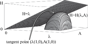
Figure 1: A schematic view of an expected form of the topological entropy spectrum $H(\lambda,A)$.

III Analysis of the 1D Bernoulli CML

III.1 Model

The map we first analyze is a Bernoulli CML, whose 2D version was originally proposed by Sakaguchi Sakaguchi-1 and its 1D version was introduced later by Kawasaki and Sasa Kawasaki_Sasa-1 . In the present work, we investigate the 1D model, which we describe below.

Figure 2: The local Bernoulli map at a site $i$. The time evolution of $\Delta_{i}^{t}$ is defined in Eq. (20).

Consider a 1-dimensional lattice which consists of $N$ lattice points $i=0,1,\cdots,N-1$. Dynamical variables $(x_{i},\Delta_{i})\in[-1,1]\times[-1,1]$ are assigned to each site $i$, and in addition, a “spin” variable $s_{i}$ is defined as

$$s_{i}\equiv\begin{cases}+1&\text{if $-1\leq x_{i}<\Delta_{i}$},\\ -1&\text{if $\Delta_{i}\leq x_{i}\leq 1$}.\end{cases}$$ (19)

With this spin, the time evolution of $(x_{i}^{t},\Delta_{i}^{t})$ is written as

$$\begin{cases}\begin{cases}x_{i}^{t+1}=f(x_{i}^{t};\Delta_{i}^{t})\equiv\dfrac{2(x_{i}^{t}+s_{i}^{t})}{1+s_{i}^{t}\Delta_{i}^{t}}-s_{i}^{t},\\ \Delta_{i}^{t+1}=\tanh\left[\dfrac{k}{2}(s_{i-1}^{t}+s_{i+1}^{t})\right],\end{cases}&\text{for odd $(i-t)$},\\ \begin{cases}x_{i}^{t+1}=x_{i}^{t},\\ \Delta_{i}^{t+1}=\Delta_{i}^{t},\end{cases}&\text{for even $(i-t)$},\end{cases}$$ (20)

with periodic boundary condition $s_{N}^{t}=s_{0}^{t}$. The updating is done alternately with respect to the parity of the site number $i$, that is to say, sites with odd $i$ are updated at even time $t$ while those with even $i$ are renewed at odd $t$. The total number of the sites $N$ is supposed to be even in order that the alternately updating rule is compatible with the periodic boundary condition. $f(x_{i}^{t};\Delta_{i}^{t})$ is a Bernoulli map, illustrated in Fig. 2. As can be seen from Eq. (20) and Fig. 2, $\Delta_{i}^{t}$ is a discrete variable and behaves as a dynamical parameter which describes the interaction between nearest-neighbor sites. Therefore, we consider only $x_{i}^{t}$ to be a dynamical variable and apply the formalism stated in the previous section. The magnitude and the tendency of the interaction are determined by the absolute value of $k$ and its sign, respectively. For positive (negative) $k$, $\Delta_{i}^{t}$ moves in the direction so as to make it more probable that the spin $s_{i}^{t}$ becomes parallel (antiparallel) to the neighboring spins, hence the interaction is ferromagnetic (antiferromagnetic).

The Bernoulli CML has several remarkable properties, as demonstrated by preceding studies Kawasaki_Sasa-1 ; Sakaguchi-1 , which should be pointed out here. First, the dynamics can be expressed in terms of the symbolic dynamics with symbols ${\bm{s}}\equiv\{s_{i}\}_{i=0}^{N-1}$. In other words, the partition $\{U_{\bm{s}}\}$ of the phase space, whose element $U_{\bm{s}}$ corresponds to a spin configuration ${\bm{s}}$, is generating and thus every orbit is specified by an infinite sequence of symbols ${\bm{s}}^{0}{\bm{s}}^{1}{\bm{s}}^{2}\cdots$. Especially, note that every UPO has a one-to-one correspondence to a finite length permutation $[{\bm{s}}]\equiv{\bm{s}}^{0}{\bm{s}}^{1}\cdots{\bm{s}}^{p-1}$. The most significant feature of the Bernoulli CML is that it respects a detailed balance and the resulting probability measure of a subset $U_{\bm{s}}$ coincides with the canonical distribution of the 1D Ising model Kawasaki_Sasa-1 ; Sakaguchi-1 , namely

$$\mu(U_{\bm{s}})\propto\exp\left(\frac{k}{2}\sum_{i=0}^{N-1}s_{i}s_{i+1}\right).$$ (21)

Therefore the Bernoulli CML can be regarded as a deterministic model of the 1D Ising (anti-)ferromagnetism in its equilibrium state and the interaction parameter $k$ corresponds to the inverse temperature. Since the marginal phase transition occurs in the 1D Ising model at the zero temperature limit, this Bernoulli CML shows a transition in the strong interaction limit $|k|\to\infty$.

III.2 Application of the thermodynamic formalism

The thermodynamic formalism in Sec. II.2 is made use of to analyze it. We adopt the Ising interaction energy per 1 spin for a macroscopic quantity

$$A({\bm{s}})\equiv-\frac{1}{N}\sum_{i=0}^{N-1}s_{i}s_{i+1}.$$ (22)

Substituting it and the Lyapunov exponent given from the slope of the function $f(x_{i}^{t};\Delta_{i}^{t})$ into Eq. (6), we can obtain the following expression of the partition function

$$Z_{q,\beta}=\sum_{\{s_{j,k}\}}\exp\left[\left(\beta+\frac{kq}{2}\right)\sum_{\text{n.n.}}s_{j,k}s_{j^{\prime},k^{\prime}}-\frac{q}{2}\left(\ln\cosh k\right)\sum_{j,k}s_{j-1,k}s_{j,k-1}-\frac{pNq}{4}\ln(4\cosh k)\right],$$ (23)

where a space-time configuration $[{\bm{s}}]$ of $N\times p$ symbols is reduced to a 2-dimensional array $\{s_{j,k}\}$ of $pN/2$ spins by exploiting the constraint $s_{i}^{t+1}=s_{i}^{t}$ for even $(i-t)$, which is outlined in Fig. 3, and $\sum_{\text{n.n.}}$ indicates a summation over all pairs of neighboring spins after the spin reduction. Equation (23) shows that, for positive $(\beta+kq/2)$ and $q$, the interaction between spins comprises helical ferromagnetic part and spatial antiferromagnetic part.

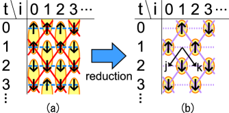
Figure 3: (Color online) A schematic illustration of the spin reduction from an UPO $[{\bm{s}}]$ to the corresponding 2-dimensional array $\{s_{j,k}\}$. (a) The spin configuration of an UPO $[{\bm{s}}]$. Spins form clusters of length $2$ in the time direction under the updating rule of Eq. (20). The red solid line and the blue broken line indicate spin interaction which comes from the Lyapunov exponent $\lambda([{\bm{s}}])$ and the observable $A([{\bm{s}}])$, respectively, in Eq. (6). (b) The 2-dimensional spin array $\{s_{j,k}\}$ obtained by the reduction, by which each cluster is reduced to a single spin located at the odd $(i-t)$. The 2 kinds of spin interaction turn into helical ferromagnetic part (purple solid line) and spatial antiferromagnetic part (purple dotted line) suppose both $(\beta+kq/2)$ and $q$ are positive.

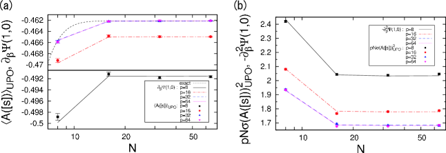
Figure 4: (Color online) Demonstration of Eqs. (9) and (10) for the 1D Bernoulli CML with $k=1$, by means of Monte Carlo calculations. Lines correspond to (a) mean $\frac{\partial\Psi}{\partial\beta}(1,0)$ and (b) standard deviation $-\frac{\partial^{2}\Psi}{\partial{\beta}^{2}}(1,0)$ at $N=8,16,32,64$ evaluated via the GMF $\Psi(q,\beta)$, which is obtained by averaging results of 400 independent Monte Carlo runs with $100,000$ samples after $100$ steps of transients. The range of errors, estimated from standard deviation among the independent runs, is less than $10^{-4}$ for (a) and $10^{-2}$ for (b), and therefore, negligible. Symbols in both figures indicate results of direct measurement of $\langle A([{\bm{s}}])\rangle_{\text{UPO}}$ and $pN\sigma(A([{\bm{s}}]))_{\text{UPO}}^{2}$, respectively, by Monte Carlo simulations with $1,000,000$ samples after $100$ steps of transients. Corresponding standard deviations are denoted by error bars. Black dashed curve in (a) represents the exact value $\langle A\rangle_{\mu}$. Note that plots for $p=32$ and $64$ are nearly at the same place. Lines and symbols for fixed $p$ and $N$ are within the range of statistical errors, and thus Eqs. (9) and (10) are confirmed. Furthermore, the two figures show that $\frac{\partial\Psi}{\partial\beta}(1,0)$ and $-\frac{\partial^{2}\Psi}{\partial{\beta}^{2}}(1,0)$ converge for sufficiently large $p$, the former of which coincides with the exact value in accordance with Eq. (9), and also for sufficiently large $N$, which indicate that the GMF $\Psi(q,\beta)$ is analytic in the limit $p,N\to\infty$.

To calculate numerically the accompanying GMF defined by Eq. (7) in the limit $p\to\infty$ with fixed $N$, or $N\to\infty$ with fixed $p$, it is well known that the zeta function method is a powerful tool to accomplish it Cvitanovic_etal-1 ; Politi_Torcini-1 . In the present analysis, however, we keep both $p$ and $N$ finite in order to maintain the formal equivalency between space and time in Eq. (23) and to exploit knowledge on the equilibrium statistical mechanics. Since the GMF has the same form as the Helmholtz free energy and we know that the GMF at physical situation is zero in systems without escape (see Eq. (8)), we adopt the computational method to calculate the difference of the free energy Frenkel-1 . From Eqs. (6) and (7), we obtain

$$\mathrm{e}^{-pN\Delta\Psi}=\left\langle\mathrm{e}^{-pN[\Delta q\lambda([{\bm{s}}])+\Delta\beta A([{\bm{s}}])]}\right\rangle_{q,\beta},$$ (24)

where $\Delta\Psi\equiv\Psi(q+\Delta q,\beta+\Delta\beta)-\Psi(q,\beta)$ and $\langle\cdots\rangle_{q,\beta}$ denotes the UPO ensemble average with the probability distribution $f([{\bm{s}}])=\mathrm{e}^{-pN[q\lambda([{\bm{s}}])+\beta A([{\bm{s}}])]}$. The evaluation of the RHS of Eq. (24) can be carried out by the Monte Carlo method, similar to that used in Kawasaki_Sasa-1 . The configuration space is a $(1+1)$-dimensional $N\times p$ lattice, each direction of which corresponds to space and time, respectively, and a spin $s_{i}^{t}=\pm 1$ is assigned to each lattice point. Then the UPO ensemble can be produced by the Metropolis algorithm with the “Hamiltonian” $pN[q\lambda([{\bm{s}}])+\beta A([{\bm{s}}])]$, or the content of the brackets in Eq. (23) for the Bernoulli CML, by which we can obtain the ensemble average and thus $\Delta\Psi$. One may think that plausible results are not available due to the exponentially increasing number of UPOs with $N$, which inevitably restricts the reachable period $p$ to be rather short. However, it does not affect since accuracy of the Monte Carlo sampling is determined by the proportion of dominant orbits in the ensemble average, which depends on the product $pN$ (see Eq. (24) and the form of $f([{\bm{s}}])$ below). That is to say, the shortness of sampled orbits can be compensated by the large number of DOFs. We can therefore compute the GMF by means of the Monte Carlo method, over a wide range of $(q,\beta)$ through the repetition of this step. Note that the step size $\Delta q$ and $\Delta\beta$ must be sufficiently small, otherwise the dominant contribution to the average is sustained by the region where $f([{\bm{s}}])$ is very small and hence a sampling during a practicable Monte Carlo run yields an inadequate result. The adequacy of Monte Carlo samplings can be checked by plotting $H(\lambda,A)$ by means of Eq. (17) and (18) and seeing that it satisfies the properties of $H(\lambda,A)$, such as $0\leq H(\lambda,A)\leq\lambda$ and the concavity. We actually confirmed in Fig. 4 that the GMF obtained in this way satisfies the relations (9) and (10).

III.3 Analysis of the phase transition

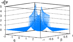
Figure 5: (Color online) The 2nd derivative of the GMF $-\frac{\partial^{2}\Psi}{\partial{\beta}^{2}}$ with $k=1,p=N=16$ in the 1D Bernoulli CML. $\Psi(q,\beta)$ is obtained from Eq. (24) with $\Delta q=0.02$ and $\Delta\beta=0.01$. The ensemble average in Eq. (24) is performed over $50,000$ Monte Carlo steps after $100$ steps discarded as transients. The derivative $\frac{\partial^{2}\Psi}{\partial{\beta}^{2}}$ is yielded by the three-point formula. The figure shown above is smoothed by taking its moving average over $5\times 5$ data points.

As is seen from Eq. (23), the 1D Bernoulli CML involves a 2-dimensional array of spins with the short-range interaction in the spatio-temporal configuration space. It suggests the occurrence of phase transitions with finite values of the parameters. It is indeed the case, which is demonstrated by varying $q$ and $\beta$ and plotting the 2nd derivative of the “free energy,” $\frac{\partial^{2}\Psi}{\partial{\beta}^{2}}$, as is shown in Fig. 5. Although we can provide no decisive statement about the occurrence of phase transitions from finite-size numerical simulations, the two sharp peaks in Fig. 5 clearly indicate it, which is confirmed by observing that they grow more acute as the system size $p$ and $N$ increases. Therefore the 1D Bernoulli CML is shown to exhibit phase transitions in the 2-dimensional space-time. These transitions, brought about by varying the temperature parameters in the thermodynamic formalism, are called q-phase transitions in the context of dynamical systems with few DOFs Hata_etal-1 . Moreover the existence of the q-phase transitions can be analytically shown in the weak-interaction limit $k\to 0$. This can be seen if we neglect $O(k^{2})$ in the argument of the exponential function in Eq. (23), namely

$$Z_{q,\beta}\simeq\left(\frac{1}{2}\right)^{pNq/2}\sum_{\{s_{j,k}\}}\exp\left[\left(\beta+\frac{kq}{2}\right)\sum_{\text{n.n.}}s_{j,k}s_{j^{\prime},k^{\prime}}\right],$$ (25)

which results in the canonical partition function of the 2D Ising model, where the presence of the 2nd order phase transition is certified Onsager-1 .

Now we mention the meaning of q-phase transitions observed in the space-time configuration space in terms of the Landau picture of continuous phase transitions. Here we do not consider the dependence on a macroscopic observable $A({\bm{x}})$ for the sake of simplicity. The rewriting to the thermodynamic formalism with $A({\bm{x}})$ is straightforward. First we expand $H(\lambda)$ around the temperature $q=q_{0}$ as follows

$$H(\lambda)\simeq H_{0}+q_{0}\lambda-\left[B(\lambda-\lambda_{0})^{2}+C(\lambda-\lambda_{0})^{4}\right],$$ (26)

where $B\geq 0$ and $C>0$ because of concavity. The minimum principle (16) yields the Lyapunov exponent at the temperature $q$, namely $\lambda(q)=\frac{\partial\Psi}{\partial q}\simeq\lambda_{0}-(q-q_{0})/2B$. Therefore the 2nd derivative of the “free energy” is $-\frac{\partial^{2}\Psi}{\partial{q}^{2}}=1/2B$, which shows that $B$ goes to zero as $q$ approaches a 2nd order q-phase transition point. Further, the probability to find a positive finite-time Lyapunov exponent per 1 DOF $\lambda$ is written as

$$P_{q}(\lambda)\propto\mathrm{e}^{-pN[q\lambda-H(\lambda)]}\propto\mathrm{e}^{-pNB[\lambda-\lambda(q)]^{2}},$$ (27)

for large $p$. Thus the occurrence of q-phase transitions involves the breakdown of the central limit theorem for finite-time Lyapunov exponents and/or finite-time average of macroscopic observable $A({\bm{x}})$. It can be understood by the fact that the correlation length and time diverge at the 2nd order transition point. Note that, as the usual Landau theory, the above statement cannot be applied at the vicinity of the transition point $2pNB^{2}\lesssim C$ Landau_Lifshitz-1 . Instead, the occurrence of q-phase transitions is ascribed to the existence of sharp corners in the function $H(\lambda)$, which implies an anomaly in the UPO distribution with respect to the Lyapunov exponent $\lambda([{\bm{x}}])$. Since UPOs form the skeleton of the chaotic invariant set Cvitanovic_etal-1 , this means a system accompanying q-phase transitions has the invariant set with a global anomalous structure. It is worth remarking that q-phase transitions in chaos with few DOFs indicate local singularities of the attractor, where hyperbolicity is lost Hata_etal-1 , whereas q-phase transitions in extended chaos treated here signify global ones, that are non-analyticities in the distribution function of UPOs, which arise without losing hyperbolicity.

The non-analyticity of the UPO distribution in the 1D Bernoulli CML can be explicitly confirmed if we consider the case $k\ll 1$, in which we can refer to the exact solution of the 2D Ising model Onsager-1 as is seen in Eq. (25). In this case, a one-to-one correspondence

$$\lambda([{\bm{s}}])\simeq\frac{1}{2}kA([{\bm{s}}])+\frac{1}{2}\log 2,$$ (28)

reduces $H(\lambda,A)$ to a univariate function $H(A)$. Note that a symbol $\simeq$ here and in Eqs. (29) and (30) below indicates that both sides of the symbol are equal as long as we neglect $O(k^{2})$. Let $Z_{\text{Ising}}$ the partition function of the 2D Ising model per 1 spin in the thermodynamic limit, namely $Z_{\text{Ising}}(J)\equiv\lim_{n\to\infty}\left[\sum_{\{s_{j,k}\}}\exp\left(J\sum_{\text{n.n.}}s_{j,k}s_{j^{\prime},k^{\prime}}\right)\right]^{1/n}$, where $n$ is the number of spins. Then we obtain from Eqs. (7), (16), (17), (25), and (28) the following relations in the limit $p,N\to\infty$:

$$A(q,\beta)\simeq-\frac{1}{2}\frac{\partial}{\partial\beta}\log Z_{\text{Ising}}(\beta+kq/2)$$

$$\phantom{A(q,\beta)}\equiv f_{A}(\beta+kq/2),$$ (29)

$$H(A)\simeq\left(\beta+\frac{kq}{2}\right)A+\frac{1}{2}\log Z_{\text{Ising}}(\beta+kq/2)$$

$$\phantom{H(A)}=f_{A}^{-1}(A)A+\frac{1}{2}\log Z_{\text{Ising}}(f_{A}^{-1}(A)),$$ (30)

where, recalling $A([{\bm{s}}])$ translates into the energy of the 2D Ising model, the function $f_{A}(x)$ is monotonic and thus its inverse is well defined. The above 2 equations give a simple relation $\frac{\partial^{2}H}{\partial{A}^{2}}=\left(\frac{\partial A}{\partial\beta}\right)^{-1}$, i.e. the reciprocal specific heat. Since the specific heat of the 2D Ising model logarithmically diverges at criticality, the 2nd derivative of $H(A)$ has a sharp corner and the 3rd derivative diverges, as are shown in Fig. 6. We can of course make the same statement on the function $H(\lambda)$ because of Eq. (28). Therefore the anomalous UPO distribution actually exists in the 1D Bernoulli CML at least for $k\ll 1$, and doubtless for all $k$, since q-phase transitions are always numerically observed.

Figure 6: The 2nd and 3rd (inset) derivatives of the “entropy function” $H(A)$ in the weak-interaction case $k\ll 1$, which indicate an anomaly in the UPO distribution of the 1D Bernoulli CML. The exact solution of the 2D Ising model Onsager-1 is used to plot these curves. Note that $H(A)$ does not depend on $k$ if we neglect $O(k^{2})$.

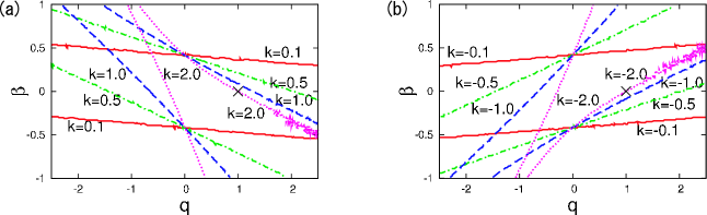
Figure 7: (Color online) q-phase transition curves of the 1D Bernoulli CML with $p=N=16$ and (a) $k=0.1,0.5,1.0,2.0,$ (b) $k=-0.1,-0.5,-1.0,-2.0$, which are indicated by a red solid line, green dot-and-dash line, blue dashed line, and purple dotted line, respectively. The black cross is located on the physical situation $(q,\beta)=(1,0)$. These transition curves are obtained by detecting local maxima of $-\frac{\partial^{2}\Psi}{\partial{\beta}^{2}}$ in $q$ and $\beta$ direction, separately, and then eliminating false maxima which come from statistical errors in the Monte Carlo samplings and the finite-size effect. They can be distinguished from rounded-off singularity by examining their continuity and dependence on the system size $p$ and $N$. See also the caption of Fig. 5 for the way to obtain $\frac{\partial^{2}\Psi}{\partial{\beta}^{2}}$. The numbers of Monte Carlo samplings are $20,000$, $20,000$, $50,000$, and $100,000$ for $|k|=0.1,0.5,1.0,2.0$ respectively.

On the other hand, as mentioned in Sec. III.1, the CML considered here is equivalent to the 1D Ising model, so that no Ising phase transition occurs at a finite value of the interaction parameter $k$. It means that, with Eqs. (9) and (10), the GMF $\Psi(q,\beta)$ in the limit $p,N\to\infty$ is analytic at the physical situation $(q,\beta)=(1,0)$ and the CML shows no q-phase transition at that point. Indeed Fig. 7 is a phase diagram for several values of $k$ and we can see that the transition curves do not go through $(q,\beta)=(1,0)$ for not so large $k$. That is, it is true that the anomalous part in the UPO distribution exists, but at finite $k$ those UPOs are hidden as non-dominant terms in the partition function $Z_{1,0}=\sum_{[{\bm{x}}]}\mathrm{e}^{-pN\lambda([{\bm{x}}])}$ and their non-analyticity is overwhelmed by the other, analytic and dominant terms. However, Fig. 7 shows that, as $|k|$ is increased and goes to infinity, the transition curves move and finally reach the physical situation. In other words the anomalous UPOs become the dominant terms, and at that moment, the Ising phase transition occurs and the non-analyticity is uncovered. This is justified by the fact that $-\frac{\partial^{2}\Psi}{\partial{\beta}^{2}}$ specifies the lower bound of the fluctuation of the Ising energy, or specific heat, so the occurrence of q-phase transition at the physical situation just means the actual Ising transition. Our consideration reveals the role of the anomalous UPO distribution as a “seed” of the Ising transition, which is ordinarily hidden. The two transition curves, observed at each $k$ in Fig. 7, correspond to the ferromagnetic (upper curve) and antiferromagnetic (lower curve) transition, respectively, which can be understood by comparing transition curves for different $k$ in Figs. 7 (a) and (b).

Finally, we add one comment on the numerical observation by Kawasaki and Sasa Kawasaki_Sasa-1 . In order to explain the reproduction of macroscopic quantities in turbulence from a single UPO 1UPO-1 , they numerically showed that the standard deviation of the Ising energy calculated from one UPO, i.e. $\sigma(A([{\bm{x}}]))_{\text{UPO}}$, goes to zero as the system size $N$ increases in the 1D Bernoulli CML. This is proved by the following facts. Since the model satisfies the scaling hypothesis (13) and it does not exhibit a q-phase transition at the physical situation for finite values of $k$, the GMF $\Psi(q,\beta)$ is assured to be well-defined and analytic in the limit $p\to\infty$ and/or $N\to\infty$. The validity of Eqs. (9) and (10) in both limits is actually suggested by means of Monte Carlo calculations as is shown in Fig. 4. Therefore, by taking the limit $N\to\infty$ in Eq. (10), we obtain $\sigma(A([{\bm{x}}]))_{\text{UPO}}\to 0$ even for a finite period $p$. This is what Kawasaki and Sasa numerically observed Kawasaki_Sasa-1 , and might be a ground for the macroscopic reproduction in turbulence 1UPO-1 . In other words, any hyperbolic extended systems which satisfy Eq. (13), or the large deviation theorem, possess this property. We can also see from Eq. (10) and Fig. 4(b) that the accuracy of a single UPO estimate, i.e. standard deviation $\sigma(A([{\bm{x}}]))_{\text{UPO}}$, asymptotically scales as $(pN)^{-1/2}$. Note that, however, the period must not be too short ($p\gtrsim 32$ in the case of the 1D Bernoulli CML) in order to regard the UPO average $\langle A([{\bm{x}}])\rangle_{\text{UPO}}$ as a good approximation of the turbulent average $\langle A\rangle_{\mu}$ (see Fig. 4 and Eq. (4)).

IV Analysis of the 1D repelling CML
-solvable case-

The UPO expansion and the thermodynamic formalism dealt with in Sec. II are also applicable to repelling systems insofar as we concentrate our attention into the dynamics on chaotic invariant sets. A modification is required only on Eq. (8), which is replaced by

$$\lim_{p\to\infty}\Psi(1,0)=\alpha,\\$$ (31)

where $\alpha$ is the escape rate per 1 DOF of the repeller, i.e. $Z_{1,0}=\sum_{[{\bm{x}}]}\mathrm{e}^{-pN\lambda([{\bm{x}}])}\sim\mathrm{e}^{-pN\alpha}$. The space-time “Hamiltonian” $pN\lambda([{\bm{x}}])$ can be now constructed at will without the strong constraint of Eq. (8), hence a solvable model is available.

Here we adopt a 1D coupled repeller map lattice introduced by Just and Schmüser Just_Schmuser-1 . Dynamical variables are $x_{i}^{t}\in I\equiv[-1,1]$ defined at each site $i=0,1,\cdots,N-1$, with a “spin” variable

$$s_{i}^{t}\equiv\operatorname{sgn}x_{i}^{t}.$$ (32)

The time evolution of $x_{i}^{t}$ is yielded by a piecewise linear map

$$x_{i}^{t+1}=f(x_{i}^{t};s_{i+1}^{t})\equiv\begin{cases}g_{-,s_{i+1}^{t}}(x_{i}^{t})&\text{if $x_{i}^{t}<0$},\\ g_{+,s_{i+1}^{t}}(x_{i}^{t})&\text{if $x_{i}^{t}>0$},\end{cases}$$ (33)

with

$$g_{-,s}(x)\equiv\begin{cases}\Gamma_{--,s}(x+c)&\text{if $-1<x\leq-c$},\\ \Gamma_{-+,s}(x+c)&\text{if $-c\leq x<0$},\end{cases}$$ (34a)

$$g_{+,s}(x)\equiv\begin{cases}\Gamma_{+-,s}(x-c)&\text{if $0<x\leq c$},\\ \Gamma_{++,s}(x-c)&\text{if $c\leq x<1$},\end{cases}$$ (34b)

for some values of slopes $\Gamma_{\pm\pm,s}>1$, as functions of the neighboring spin $s$, and a constant $0<c<1$. The periodic boundary condition $s_{N}^{t}=s_{0}^{t}$ is considered to close the definition. The local map defined in this way is sketched in Fig. 8. The invariant set of this CML can be symbolized again via the partition

$$V_{\bm{s}}\equiv g_{s_{0},s_{1}}^{-1}(I)\times g_{s_{1},s_{2}}^{-1}(I)\times\cdots\times g_{s_{N-1},s_{0}}^{-1}(I),$$ (35)

where the local partition $g_{s_{i},s_{i+1}}^{-1}(I)$ is depicted in Fig. 8. Hence the first and second symbol in the subscripts of $\Gamma_{\pm\pm,s}$ indicate a spin of site $i$ at time $t$ and $t+1$ respectively.

Figure 8: The local map, given by Eqs. (33) and (34), for the repelling CML by Just and Schmüser. $\Gamma_{\pm\pm,s_{i+1}^{t}}$ indicates a slope of each piecewise linear part.

Now we apply the thermodynamic formalism to the model. The slopes $\Gamma_{s_{i}^{t}s_{i}^{t+1},s_{i+1}^{t}}$, which prescribe both the local dynamics and the interaction between neighboring sites, can be chosen arbitrarily provided that the local map does not cross the boundary $x=0,\pm 1$. Here we choose the simplest form after Just and Schmüser Just_Schmuser-1 ,

$$\Gamma_{s_{i}^{t}s_{i}^{t+1},s_{i+1}^{t}}=\exp\left[-Js_{i}^{t}\left(s_{i}^{t+1}+s_{i+1}^{t}\right)+e_{0}\right],$$ (36)

where $J$ and $e_{0}$ are some constants. A macroscopic quantity is set to be the Ising energy again, namely Eq. (22). Thus, the partition function (6) for this model is calculated as

$$Z_{q,\beta}=\sum_{[{\bm{s}}]}\exp\left\{\sum_{i=0}^{N-1}\sum_{t=0}^{p-1}\left[(qJ+\beta)s_{i}^{t}s_{i+1}^{t}+qJs_{i}^{t}s_{i}^{t+1}\right]\\ -pNqe_{0}\right\},$$ (37)

which is nothing but the canonical partition function for the 2D Ising model on the square lattice with anisotropic interaction. Note that the Bernoulli CML treated in the previous section results in the 2D Ising model only at the weak interaction limit, whereas for the repelling CML it holds for all $q$ and $\beta$. By setting $(q,\beta)=(1,0)$, i.e. physical situation, in Eq. (37), the model turns out to show the 2D Ising transition at $J=J_{c}\equiv\frac{1}{2}\ln(1+\sqrt{2})$ as is shown in Just_Schmuser-1 . Moreover, the existence and location of the q-phase transition curve $(q_{c},\beta_{c})$ is also given exactly by Onsager’s celebrated paper Onsager-1 as

$$\beta_{c}=\frac{1}{2}\operatorname{Arcsinh}\left[1/\sinh(2q_{c}J)\right]-q_{c}J.$$ (38)

Figure 9 shows its phase diagram for several values of the coupling constant $J$. In this case, the transition curve passes the physical situation $(q,\beta)=(1,0)$ linearly as $J$ goes through $J_{c}$, which can be explicitly written from Eq. (38) as

$$\beta_{c}\simeq-2(J-J_{c}), q_{c}$$ for fixed , (39a)

$$q_{c}\simeq 1-(J-J_{c})/J_{c}, \beta_{c}$$ for fixed . (39b)

This linear dependence of the q-phase transition point $(q_{c},\beta_{c})$ on the control parameter $J$ at the vicinity of the actual phase transition point $J=J_{c}$ results from the fact that the transition observed here is not a marginal one. Hence this relation between the two transition points is expected to be general.

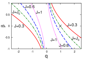
Figure 9: (Color online) q-phase transition curves (38) of the 1D repelling CML defined by Eqs. (32)-(34) and (36), with $J=0.3,J_{c}\approx 0.44,0.6,1.0$, which are drawn with a red solid line, green dot-and-dash line, blue dashed line, and purple dotted line, respectively. The black cross indicates the physical situation $(q,\beta)=(1,0)$. The transition curves for negative $J$ are obtained by reflecting the figure over $q$- or $\beta$-axis.

On the anomalous structure of the invariant set with respect to the UPO distribution and its role in the occurrence of the phase transition, the same statement as the previous section holds, which can be demonstrated directly for this model since the rigorous solution is available.

V Discussion

The intimate relation between q-phase transitions and phase transitions in the sense of statistical mechanics is investigated on the basis of the thermodynamic formalism and the UPO expansion. Since mathematically the partition function (6) has the identical form to that of the canonical statistical mechanics with $q$ and $\beta$ as inverse temperature, many useful relations in equilibrium physics, such as Eqs. (9), (10), and (17), also hold in extended chaotic systems, which can be far from equilibrium. Although similar relations have been already pointed out for dynamical systems with few DOFs by several authors Fujisaka_Inoue-1 ; Cvitanovic_etal-1 ; Hata_etal-1 , we reconstructed it for extended systems with concerning the number of DOFs $N$ explicitly. By that means the analogy is kept with the equilibrium statistical mechanics of several-dimensional systems. A richer harvest may be reaped from it, as long as attention is paid to the strict constraint of Eq. (8) for systems without escape.

As regards phase transitions, anomalously distributed UPOs turn out to be responsible, which show sharp corners in the distribution function and can be visualized in terms of q-phase transition. The anomalous part exists in systems with transitions, over the range of control parameters where the topological structure of an attractor does not change. It is ordinarily hidden as non-dominant terms in the partition function $Z_{1,0}$ and no critical behavior is observed there. The actual transition occurs when the control parameters are varied, the UPO distribution is changed and finally the anomalous UPOs become a dominant part. In this sense we call the anomalous part of the UPO distribution “seed” of phase transitions.

One question may arise here: “What brings this anomalous UPO distribution to dynamical systems with phase transitions?” The answer is clear for the two Ising-like systems considered in this paper, where the origin of phase transitions is by construction well known from the knowledge of equilibrium statistical mechanics: the competition between interaction energy and entropy is relevant. Taking ferromagnet for example, the free energy $F(E)=E-TS(E)$ calculated under some fixed energy is increased by low entropy for strongly ferromagnetic configurations (corresponding to low $E$), while it is raised by high internal energy for strongly paramagnetic configurations (corresponding to high $E$). It means there are intermediate configurations where the two mechanisms compete. In fact, this competition occurs at one point, i.e. at some specific value of $E$, in the thermodynamic limit, which brings a sharp corner to the functional form of $S(E)$. Then the phase transition occurs at a temperature which minimizes the free energy at that point.

The role of UPOs in q-phase transitions — not in actual phase transitions — is exactly the same as that of microstates which we have seen above. That is, the anomalous distribution of UPOs results from the competition between average positive Lyapunov exponent and topological entropy. This mechanism may be widespread even among “natural” extended chaotic systems, because it is reasonable to expect that the number of UPOs with plenty of large Lyapunov exponents is very small, and that it grows in the same manner as equilibrium microstates (see Eq. (13) and Ref. Beck-1 ; Kubo-1 ). Note that the existence of symbolic dynamics is also not required, since the underlying basis described in Sec. II is constructed generally for hyperbolic maps.

Taking into account the above considerations and the aforesaid similarities in statistics of macroscopic observables such as Eqs. (9) and (10), we can propose a definition of phase transitions and their order in extended dynamical systems in the Ehrenfest’s sense: phase transitions are associated with the singularity of the GMF at the physical situation $(q,\beta)=(1,0)$. The transition can be said to be of $n$-th order if an $n$-th derivative of the GMF with respect to $q$ or $\beta$ does not exist or has a discontinuity, and hence the system is accompanied by $n$-th order q-phase transition. This is a mathematically simple-minded statement as well as that based on the non-uniqueness of a natural measure. Moreover it is worth remarking that the proposed definition can clearly characterize both first and higher order transitions, while definitions in the Gibbsian sense have some ambiguity when it comes to treat higher order transitions. Though the new definition has also several problems which will be mentioned later, it can be used to classify phase transitions out of equilibrium and to investigate their nature further. This is the main proposition of this paper.

The second outcome is on the propriety of treating locally defined control parameters as macroscopic “temperature.” As we have seen in Sec. III and IV, systems which exhibit a phase transition have an anomalous UPO distribution, the position of whose non-analytic part is specified by critical nominal temperatures $q_{c}$ and $\beta_{c}$. Therefore, our observation that they vary with local control parameters means that a change in local parameters leads to a change in “macroscopic temperature” through the non-analyticity of the UPO distribution. This macroscopic temperature actually takes part in phase transitions, since it crosses through the physical situation $(q,\beta)=(1,0)$ when a transition occurs, and since it mathematically works in the same way as real temperature in equilibrium systems (cf. Eqs. (6), (9), and (10)).

Let us then discuss the replacement of “temperature” by local control parameters around transition points. Let $P$ denote some control parameter in an extended dynamical system with a phase transition. As we have already seen in Sec. IV, the relation between parameter $P$ and q-phase transition point $(q_{c},\beta_{c})$ at the vicinity of the transition point $P=P_{c}$ is expected to be linearly dependent

$$\beta-\beta_{c}\simeq C_{1}(P-P_{c}), q_{c}$$ for fixed , (40a)

$$q-q_{c}\simeq C_{2}(P-P_{c}), \beta_{c}$$ for fixed , (40b)

for transitions which are not marginal. Here we set $q$ and $\beta$ at the physical situation $(q,\beta)=(1,0)$. Therefore, as far as some universal relation in equilibrium physics is concerned which is not affected by microscopic details of models, e.g. critical behavior, the same relation may hold in extended chaotic systems by replacing inverse temperature $(1/k_{B}T-1/k_{B}T_{c})$ with $C_{1}(P-P_{c})$. A similar statement could be also said on the positive Lyapunov exponent per 1 DOF, in which case Eq. (40b) is used for the replacement. Conditions which should be satisfied at least by the relation are that (1) it is about some macroscopic quantities obtained by differentiating a free energy, and that (2) its mathematical expression itself is insensitive to variations in the control parameter $P$. The difference in the relation between 2nd or higher order moments and derivatives of the “free energy” from its counterpart in equilibrium statistical mechanics might also have an influence — in extended chaos the derivatives can only tell the lower bound of the corresponding moments due to temporal correlation, as is seen in Eq. (10) —. Provided that those restrictions are taken into consideration, we believe that the mentioned replacement can be applied to a wide range of extended systems. Note that universal scaling relations in critical behavior satisfy the above conditions and thus corresponding critical exponents are likely to be kept invariant under the replacement of temperature $T$ by the local control parameter $P$. It can be a basis on which scaling relations indeed work under such a replacement in some high-dimensional chaotic systems (e.g. Marcq_Chate_Manneville-2 ; Marcq_Chate_Manneville-1 ).

In order to justify the above arguments on a rigid basis, several problems need to be clarified. To begin with, it is unclear in extended chaotic systems how common the existence of the anomalous UPO distribution is, and also how prevalent its relation to phase transitions is. The latter is especially important, since it involves a change in the UPO distribution and thus there is no counterpart in equilibrium statistical mechanics. Further studies are crucial.

From a fundamental point of view, we do not mathematically care in this paper either the existence of the two limits $p\to\infty$ and $N\to\infty$, their order or the fact that they do not commute. They are undoubtedly important in order to argue spatio-temporal chaos on the mathematically proper basis MathReviews-1 ; Gielis_MacKay-1 ; Blank_Bunimovich-1 ; Bardet_Keller-1 ; Bricmont_Kupiainen-1 . An examination of the behavior of infinite-size systems requires that we first take the limit $N\to\infty$ and then $p\to\infty$, at variance with usual statistical mechanics where the limit is taken over sizes of all dimensions simultaneously. This may be the reason why some extended chaotic systems defined in $d$-dimensional space show critical behaviors of $d$-dimensional universality classes despite the corresponding $(d+1)$-dimensional configuration space Marcq_Chate_Manneville-1 . The problem of the incommutability should be considered seriously, since the definition of phase transitions by means of the singularity of the GMF involves both the limit $p,N\to\infty$.

Another problem is on the arbitrariness for the choice of a macroscopic quantity $A({\bm{x}})$ when we deal with q-phase transitions with respect to $\beta$. There is no clear criterion for it, except for that $A({\bm{x}})$ must be affected by phase transitions : its expectation value or fluctuation must show a discontinuity or divergence. An order parameter of the considered transition is a candidate. In our examples in Sec. III and IV, however, we adopted the quantity which can be regarded as energy on the analogy with equilibrium spin systems. The relation between the choice for $A({\bm{x}})$ and the behavior of q-phase transition curves near critical points remains to be clarified, especially about their linear dependence on control parameters such as Eq. (40).

In conclusion, the old concept of the thermodynamic formalism and the periodic orbit expansion turns out to be useful to characterize phase transitions in extended dynamical systems. Theoretically, one possible definition of phase transitions is proposed, which is complementary to the usual definition in terms of a change in the number of natural measures. It can be used to classify and examine non-equilibrium transitions in chaotic systems, especially higher order transitions, with the help of a suitable technique to generate or approximate the UPO ensemble. Recently developed method such as Ref. Lan_Cvitanovic-1 ; Sasa_Hayashi-1 might be applied for this purpose. With regard to experiments and numerical simulations, a ground is obtained on which we can sometimes treat an externally imposed control parameter as macroscopic “temperature” around phase transition points. Although some significant problems are left for future studies, this assertion is expected to support discussions on universality classes in non-equilibrium systems from real and numerical experiments.