The dynamical spin structure factor for the anisotropic spin-$1/2$ Heisenberg chain

Abstract

The longitudinal spin structure factor for the $XXZ$-chain at small wave-vector $q$ is obtained using Bethe Ansatz, field theory methods and the Density Matrix Renormalization Group. It consists of a peak with peculiar, non-Lorentzian shape and a high-frequency tail. We show that the width of the peak is proportional to $q^{2}$ for finite magnetic field compared to $q^{3}$ for zero field. For the tail we derive an analytic formula without any adjustable parameters and demonstrate that the integrability of the model directly affects the lineshape.

One of the seminal models in the field of strong correlation effects is the antiferromagnetic spin-$1/2$ $XXZ$-chain

$$H=J\sum_{j=1}^{N}\left[S_{j}^{x}S_{j+1}^{x}+S_{j}^{y}S_{j+1}^{y}+\Delta S_{j}^{z}S_{j+1}^{z}-hS_{j}^{z}\right]\;,$$ (1)

where $J>0$ is the coupling constant and $h$ a magnetic field. The parameter $\Delta$ describes an exchange anisotropy and the model is critical for $-1<\Delta\leq 1$. Recently, much interest has focused on understanding its dynamics, in particular, the spin Zotos (1999) and the heat conductivity Klümper and Sakai (2002), both at wave-vector $q=0$. A related important question refers to dynamical correlation functions at small but nonzero $q$, in particular the dynamical spin structure factors $S^{\mu\mu}(q,\omega)$, $\mu=x,y,z$ Müller et al. (1981). These quantities are in principle directly accessible by inelastic neutron scattering. Furthermore, they are important to resolve the question of ballistic versus diffusive transport raised by recent experiments Thurber et al. (2001) and would also be useful for studying Coulomb drag for two quantum wires Pustilnik et al. (2003).

In this letter we study the lineshape of the longitudinal structure factor $S^{zz}(q,\omega)$ at zero temperature in the limit of small $q$. Our main results can be summarized as follows: By calculating the form factors $F(q,\omega)\equiv\left\langle 0\left|S_{q}^{z}\right|\alpha\right\rangle$ (here $|0\rangle$ is the ground state and $|\alpha\rangle$ an excited state) for finite chains based on a numerical evaluation of exact Bethe Ansatz (BA) expressions Kitanine et al. (1999); Caux and Maillet (2005) we establish that $S^{zz}(q,\omega)$ consists of a peak with peculiar, non-Lorentzian shape centered at $\omega\sim vq$, where $v$ is the spin-wave velocity, and a high-frequency tail. We find that $|F(q,\omega)|$ is a rapidly decreasing function of the number of particles involved in the excitation. In particular, we find for all $\Delta$ that the peak is completely dominated by two-particle (single particle-hole) and the tail by four-particle states (denoted by 2$p$ and 4$p$ states, respectively). Including up to eight-particle as well as bound states we verify using Density Matrix Renormalization Group (DMRG) that the sum rules are fulfilled with high accuracy corroborating our numerical results. By solving the BA equations for small $\Delta$ and infinite system size analytically we show that the width of the peak scales like $q^{2}$ for $h\neq 0$. Furthermore, we calculate the high-frequency tail analytically based on a parameter-free effective bosonic Hamiltonian. We demonstrate that our analytical results for the linewidth and the tail are in excellent agreement with our numerical data.

For a chain of length $N$ the longitudinal dynamical structure factor is defined by

$$S^{zz}\left(q,\omega\right) = \frac{1}{N}\sum_{j,j^{\prime}=1}^{N}e^{-iq\left(j-j^{\prime}\right)}\int_{-\infty}^{+\infty}\!\!\!\!\!\!\!\!dt\,e^{i\omega t}\left\langle S_{j}^{z}\left(t\right)S_{j^{\prime}}^{z}\left(0\right)\right\rangle$$ (2)

$$= \frac{2\pi}{N}\sum_{\alpha}\left|\left\langle 0\left|S_{q}^{z}\right|\alpha\right\rangle\right|^{2}\delta\left(\omega-E_{\alpha}\right)\;.$$

Here $S_{q}^{z}=\sum_{j}S_{j}^{z}e^{-iqj}$ and $\left|\alpha\right\rangle$ is an eigenstate with energy $E_{\alpha}$ above the ground state energy. For a finite system, $S^{zz}\left(q,\omega\right)$ at fixed $q$ is a sum of $\delta$-peaks at the energies of the eigenstates. In the thermodynamic limit $N\rightarrow\infty$, the spectrum is continuous and $S^{zz}\left(q,\omega\right)$ becomes a smooth function of $\omega$ and $q$. By linearizing the dispersion around the Fermi points and representing the fermionic operators in terms of bosonic ones the Hamiltonian (1) at low energies becomes equivalent to the Luttinger model Giamarchi (2004). For this free boson model $S^{zz}(q,\omega)$ can be easily calculated and is given by

$$S^{zz}\left(q,\omega\right)=K\left|q\right|\delta\left(\omega-v\left|q\right|\right)\,,$$ (3)

where $K$ is the Luttinger parameter. This result is a consequence of Lorentz invariance: a single boson with momentum $\left|q\right|$ always carries energy $\omega=v|q|$, leading to a $\delta$-function peak at this level of approximation.

We expect the simple result (3) to be modified in various ways. First of all, the peak at $\omega\sim vq$ should acquire a finite width $\gamma_{q}$. The latter can be easily calculated for the $XX$ point, $\Delta=0$, where the model is equivalent to non-interacting spinless fermions. In this case the only states that couple to the ground state via $S^{z}_{q}$ are those containing a single particle-hole excitation (2$p$ states). As a result, the exact $S^{zz}(q,\omega)$ is finite only within the boundaries of the 2$p$ continuum. For $h\neq 0$, one finds $\gamma_{q}\approx q^{2}/m$ for small $q$, where $m=(J\cos k_{F})^{-1}$ is the effective mass at the Fermi momentum $k_{F}$. For $h=0$, $m^{-1}\to 0$ and the width becomes instead $\gamma_{q}\approx Jq^{3}/8$. In both cases the non-zero linewidth is associated with the band curvature at the Fermi level and sets a finite lifetime for the bosons in the Luttinger model. Different attempts to calculate $\gamma_{q}$ for $\Delta\neq 0$ have focused on perturbation theory in the band curvature terms Samokhin (1998) or in the interaction $\Delta$ Pirooznia and Kopietz (2005); Teber (2006) and contradictory results were found. All these approaches have to face the breakdown of perturbation theory near $\omega\sim vq$.

Since perturbative approaches show divergences on shell, our discussion about the broadening of the peak is based on the BA solution. The BA allows us to calculate the energy of an eigenstate exactly from a system of coupled non-linear equations Takahashi (1999). For $\Delta=0$ these equations decouple, the structure factor is determined by 2$p$ states only and one recovers the free fermion solution. For $|\Delta|\ll 1$ the most important excitations are still of the 2$p$ type and one can obtain the energies of these eigenstates analytically in the thermodynamic limit by expanding the BA equations in lowest order in $\Delta$. For $h\neq 0$ (i.e., finite magnetization $s\equiv\left\langle S_{j}^{z}\right\rangle$) this leads to

$$\gamma_{q}=4J\left(1+\frac{2\Delta}{\pi}\sin k_{F}\right)\cos k_{F}\sin^{2}\frac{q}{2}\approx\frac{q^{2}}{m^{*}}\;.$$ (4)

for the 2$p$ type excitations. We therefore conclude that the interaction does not change the scaling of $\gamma_{q}$ compared to the free fermion case but rather induces a renormalization of the mass given by $m\rightarrow m^{*}=m/(1+2\Delta\sin k_{F}/\pi)$. We have verified our analytical small $\Delta$ result by calculating the form factors numerically Caux and Maillet (2005). For all $\Delta$, we find that excitations involving more than two particles have negligible spectral weight in the peak region. In Fig. 1 we therefore show only the form factors for the 2$p$ states and a typical set of parameters.

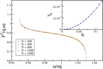
Figure 1: (Color online) Form factors squared for the 2$p$ excitations and different $N$ at $\Delta=0.25$, $s=-0.1$ and $q=2\pi/25$. The inset shows the scaling of the width $\gamma_{q}$. The points are obtained by an extrapolation $N\to\infty$ of the numerical data. The solid line is the prediction (4), $\gamma_{q}=0.356\,q^{2}$.

The form factors, for different chain lengths, $N$, collapse onto a single curve determining the lineshape of $S^{zz}(q,\omega)$ except for a high-frequency tail discussed later. The form factors are enhanced near the lower threshold $\omega_{L}(q)$ and suppressed near the upper threshold $\omega_{U}(q)$ in contrast to the almost flat distribution for $\Delta=0$. The lineshape agrees qualitatively with the recent result in Pustilnik et al. (2006) predicting a power-law singularity at $\omega_{L}(q)$ with a $q$- and $\Delta$-dependent exponent. The inset of Fig. 1 provides a numerical confirmation that $\gamma_{q}\sim q^{2}$, with the correct pre-factor as predicted in (4) for $k_{F}=2\pi/5$. For zero field, the bounds of the 2$p$ continuum are known analytically des Cloizeaux and Gaudin (1966) and lead to a scaling $\gamma_{q}\sim q^{3}$ for $-1<\Delta\leq 1$. Furthermore, for $h=0$ and $\Delta=1$, an exact result for the 2$p$ contributions to the structure factor has been derived Karbach et al. (1997).

Calculating a small number of form factors for finite chains poses two important questions: 1) For finite chains $S^{zz}(q,\omega)$ at small $q$ is dominated by 2$p$ excitations. Is this still true in the thermodynamic limit? 2) How much of the spectral weight does the relatively small number of form factors calculated account for? We can shed some light on these questions by considering the sum rule $I(q)=(2\pi)^{-1}\int d\omega\,S^{zz}(q,\omega)=N^{-1}\langle S^{z}_{q}S^{z}_{-q}\rangle$ where the static correlation function can be obtained by DMRG. As example, we consider again $\Delta=0.25$, $s=-0.1$, $q=2\pi/25$ with $N=200$. For this case we have calculated $2,220,000$ form factors including up to $8p$ excited states as well as bound states. Note, however, that this is still small compared to a total number of states of $2^{200}$. In the DMRG up to $2400$ states were kept and the ordinary two-site method was utilized but with corrections to the density matrix to ensure good convergence with periodic boundary conditions White (1999). The typical truncation error was then $\sim 10^{-10}$ and within the accuracy of the DMRG calculation (3 parts in $10^{5}$) the $2,220,000$ form factors account for 100% of $I(q)$. 99.97% of the spectral weight is concentrated in $I_{2}(q)$, the contribution caused by the $qN/2\pi=8$ single particle-hole type excitations at $\omega\sim vq$. With increasing $N$ we observe an extremely slow decrease in $I_{2}(q)$; however, even for a system of $2400$ sites, $I_{2}(q)$ is only reduced by 0.13% compared to the $N=200$ case. While this large $N$ behavior definitely requires further investigation it may not be very relevant to experiments, where effective chain lengths are limited by defects.

Another feature missed in (3) is the small spectral weight extending up to high frequencies $\omega\sim J$. This is relevant in the context of drag resistance in quantum wires because of the equivalence of $S^{zz}(q,\omega)$ and the density-density correlation function for spinless fermions Pustilnik et al. (2003). To calculate the high-frequency tail we start from the Luttinger model

$$\mathcal{H}_{LL}=\frac{v}{2}\left[\Pi^{2}+\left(\partial_{x}\phi\right)^{2}\right]\,.$$ (5)

Here, $\phi(x)$ is a bosonic field and $\Pi(x)$ its conjugated momentum satisfying $[\phi(x),\Pi(y)]=i\delta(x-y)$. The slowly varying part of the spin operator is expressed as $S^{z}_{j}\sim\sqrt{K/\pi}\,\partial_{x}\phi$. Note that both $v$ and $K$ depend on $\Delta$ and $h$. In the language of the Luttinger model, the spectral weight at high frequencies is made possible by boson-boson interactions. Therefore, we add to the model (5) the following terms

$$\delta\mathcal{H}(x) = \eta_{-}\left[\left(\partial_{x}\phi_{L}\right)^{3}-\left(\partial_{x}\phi_{R}\right)^{3}\right]$$ (6)

$$+ \eta_{+}\left[\left(\partial_{x}\phi_{L}\right)^{2}\partial_{x}\phi_{R}-\left(\partial_{x}\phi_{R}\right)^{2}\partial_{x}\phi_{L}\right]$$

$$+ \zeta_{-}\left[(\partial_{x}\phi_{L})^{4}+(\partial_{x}\phi_{R})^{4}\right]+\zeta_{+}(\partial_{x}\phi_{L})^{2}(\partial_{x}\phi_{R})^{2}$$

$$+ \zeta_{3}\left[\partial_{x}\phi_{L}(\partial_{x}\phi_{R})^{3}+\partial_{x}\phi_{R}(\partial_{x}\phi_{L})^{3}\right]$$

$$+ \lambda\cos\left(4\sqrt{\pi K}\phi+4k_{F}x\right)\;,$$

where $\phi_{R,L}$ are the right- and left-moving components of the bosonic field with $\phi=(\phi_{L}-\phi_{R})/\sqrt{2}$. They obey the commutation relations $[\partial_{x}\phi_{L,R}(x),\partial_{x}\phi_{L,R}(y)]=\mp i\partial_{y}\delta(x-y)$. These are the leading irrelevant operators stemming from band curvature and the interaction part. The amplitudes $\eta_{\pm}$, $\zeta_{\pm}$, $\zeta_{3}$ and $\lambda$ are functions of $\Delta$ and $h$. For $h\neq 0$ the $\lambda$-term (Umklapp term) is oscillating and can therefore be omitted at low energies. Besides, the $\zeta$-terms have a higher scaling dimension than the $\eta_{\pm}$-terms, so the latter yield the leading corrections. For $h=0$, on the other hand, particle-hole symmetry dictates that $\eta_{\pm}=0$ and we must consider the $\zeta$-terms as well as the Umklapp term. For $\gamma_{q}\ll\omega-v\left|q\right|\ll J$ it is safe to use finite order perturbation theory in these irrelevant terms.

In the finite field case the tail is due to the $\eta_{+}$-interaction. This allows for intermediate states with one right- and one left-moving boson, which together can carry small momentum but high energy $\omega\gg v\left|q\right|$. It is convenient to write the structure factor defined in (2) as $S^{zz}(q,\omega)=-2\,\mbox{Im}\,\chi^{ret}(q,\omega)$ where $\chi^{ret}=-(K/\pi)\langle\partial_{x}\,\phi\partial_{x}\phi\rangle$ is the retarded spin-spin correlation function. The correction at lowest order in $\eta_{+}$ to the free boson result then reads

$$\!\!\!\!\!\!\!\delta\chi\left(q,i\omega_{n}\right)=\left[D_{R}^{\left(0\right)}\left(q,i\omega_{n}\right)+D_{L}^{\left(0\right)}\left(q,i\omega_{n}\right)\right]^{2}\Pi_{RL}\left(q,i\omega_{n}\right)$$

$$\Pi_{RL}\left(q,i\omega_{n}\right)=-\frac{2K\eta_{+}^{2}}{\pi}\int\int dxd\tau e^{-i(qx-\omega_{n}\tau)}$$ (7)

$$\quad\quad\quad\quad\quad\quad\times D_{R}^{\left(0\right)}\left(x,\tau\right)D_{L}^{\left(0\right)}\left(x,\tau\right).$$

where $D_{R,L}^{(0)}(q,i\omega_{n})=\langle\partial_{x}\phi_{L,R}\,\partial_{x}\phi_{L,R}\rangle=\pm|q|/(i\omega_{n}\mp v|q|)$ are the free boson propagators for the right- and left-movers, respectively, and $\Pi_{RL}\left(q,i\omega_{n}\right)$ is the self-energy. The tail of $S^{zz}(q,\omega)$ for $h\neq 0$ is then given by

$$\delta S^{zz}_{\eta_{+}}\left(q,\omega\right)=\frac{K\eta_{+}^{2}q^{4}}{v\pi}\,\frac{\theta\left(\omega-v\left|q\right|\right)}{\omega^{2}-v^{2}q^{2}}.$$ (8)

For $h=0$ a connection between the integrability of the $XXZ$-model and the parameters in the corresponding low-energy effective theory exists Bazhanov et al. (1997). The integrability is related to an infinite set of conserved quantities where the first nontrivial one is the energy current defined by $J_{E}=\int dx\,j_{E}(x)$ with $\partial_{x}\,j_{E}(x)=i[\mathcal{H}(x),\int dy\mathcal{H}(y)]$ Zotos et al. (1997). For the Hamiltonian (6) we find

$$j_{E} = -\frac{v}{2}\left[(\partial_{x}\phi_{L})^{2}-(\partial_{x}\phi_{R})^{2}\right]-4\zeta_{-}\left[(\partial_{x}\phi_{L})^{4}-(\partial_{x}\phi_{R})^{4}\right]$$ (9)

$$+ 2\zeta_{3}\left[\partial_{x}\phi_{L}(\partial_{x}\phi_{R})^{3}-\partial_{x}\phi_{R}(\partial_{x}\phi_{L})^{3}\right]+\ldots\;,$$

where the neglected terms contain more than four derivatives. Now conservation of the energy current, $[J_{E},H]=0$, implies $\zeta_{3}=0$ . The spectral weight at high frequencies is therefore given by the $\zeta_{+}$ and $\lambda$-terms only.

The perturbation theory for the $\zeta_{+}$-term is analogous to the one for the $\eta_{+}$-term. Now the incoming left (right) boson can decay into one left (right) and two right (left) bosons. This contribution is then given by

$$\delta S^{zz}_{\zeta_{+}}\left(q,\omega\right)=\frac{K\zeta_{+}^{2}}{48\pi^{2}v^{3}}q^{2}(\omega^{2}-v^{2}q^{2})\theta(\omega-v|q|)\;.$$ (10)

For the Umklapp term, we calculate the correlations following Schulz (1986) and find

$$\delta S^{zz}_{\lambda}\left(q,\omega\right)=Aq^{2}(\omega^{2}-v^{2}q^{2})^{4K-3}\theta(\omega-v|q|)\;,$$ (11)

where $A=8\pi^{2}\lambda^{2}K^{2}(2v)^{3-8K}/\Gamma^{2}(4K)$. We remark that, in a more general non-integrable model, the $\zeta_{3}$ term in Eq. (6) leads to an additional contribution to the tail which decreases with energy and becomes large near $\omega\sim vq$. The increasing tail found in the integrable case implies a non-monotonic behavior of $S^{zz}(q,\omega)$. Eqs. (8), (10) and (11) are valid in the thermodynamic limit. We can extend these results for finite systems and express them in terms of the form factors appearing in (2). For a given momentum $q=2\pi n/N$, the form factors generated by integer dimension operators as in (8) and (10) will then be situated at the discrete energies $\omega_{l}=2\pi vl/N$ with $l=n+2,n+4,\cdots$. The form factors belonging to (11), on the other hand, will have energies $\omega_{l}=2\pi v(l+4K)/N$ with $l=n,n+2,\cdots$.

To compare our field theory results for the tail with BA data for the form factors we have to determine the a priori unknown parameters in the effective Hamiltonian (6). In general, they can only be obtained in terms of a small-$\Delta$ expansion. To lowest order in $\Delta$, Eq. (8) reduces to the weakly interacting result in Pustilnik et al. (2003); Teber (2006). We also checked that in this limit $\zeta_{3}=0$ for the $XXZ$-model but $\zeta_{3}$ becomes finite if we introduce a next-nearest neighbor interaction that breaks integrability. For an integrable model the coupling constants can be determined by comparing thermodynamic quantities accessible by BA and field theory. Lukyanov Lukyanov (1998) used this procedure to find a closed form for $\zeta_{\pm}$ and $\lambda$ in the case $h=0$. Similarly, the parameters $\eta_{\pm}$ can be related to the change in $v$ and $K$ when varying $h$ and we find $J\eta_{-}(h_{0})=\sqrt{2\pi/K}v^{2}(a+b/2)/6$ and $J\eta_{+}(h_{0})=\sqrt{2\pi/K}v^{2}b/4$ where $a=v^{-1}\partial v/\partial h|_{h=h_{0}}$ and $b=K^{-1}\partial K/\partial h|_{h=h_{0}}$. A numerical solution of the BA integral equations for $v$, $K$ for infinite system size then allows us to fix $\eta_{\pm}$ accurately for all anisotropies and fields so that the formulas for the tail do not contain any free parameters. The comparison with the form factors computed by BA for finite and zero field is shown in Figs. 2 and 3, respectively. We note that the energies of the eigenstates are actually nondegenerate and spread around the energy levels predicted by field theory (see inset of Fig. 2).

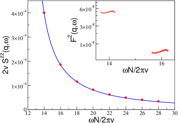
Figure 2: (Color online) Form factors (dots) obtained by BA compared to formula (8) (line) for $\Delta=0.75$, $s=-0.1$, $N=600$ and $q=2\pi/50$. The form factors for the exact eigenstates at $\omega\approx 2\pi vl/N$ are added and represented as a single point. The inset shows each form factor separately. The number of states at each level agrees with a simple counting based on multiple particle-hole excitations created around the Fermi points.

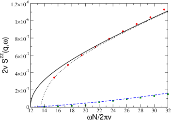
Figure 3: (Color online) Sum of form factors at $\omega\approx 2\pi v(l+4K)/N$ (dots) and at $\omega\approx 2\pi vl/N$ (squares) obtained by BA for $\Delta=0.25$, $s=0$, $N=600$ and $q=2\pi/50$. The solid line corresponds to (11), the dotted line to (11) with finite size corrections included Note (1999), and the dashed line to (10).

In summary, we have presented results for the lineshape of $S^{zz}(q,\omega)$ for small $q$ based on a numerical evaluation of form factors for finite chains. We established a linewidth $\gamma_{q}\sim q^{2}$ for $h\neq 0$ by solving the BA equations analytically for small $\Delta$. In addition, we showed that the spectral weight for frequencies $\gamma_{q}\ll\omega-v\left|q\right|\ll J$ is well described by the effective bosonic Hamiltonian. We presented evidence that the lineshape of $S^{zz}(q,\omega)$ depends on the integrability of the model. This becomes manifest in the field theory approach by a fine tuning of coupling constants and the absence of certain irrelevant operators.