Sound Velocity and Meissner Effect in Light-heavy Fermion Pairing Systems

Abstract

In the frame of a four fermion interaction theory, we investigated the collective excitation in light-heavy fermion pairing systems. When the two species of fermions possess different masses and chemical potentials but keep the same Fermi surface, we found that the sound velocity in superfluids and the inverse penetration depth in superconductors have the same mass ratio dependence as the ratio of the transition temperature to the zero temperature gap.

The study on Cooper pairing between fermions with different masses promoted great interest both theoretically and experimentally in recent years. A new pairing phenomenon, the breached pairing or interior gap, was proposed in the study of light-heavy fermion pairing systemsBP1 ; BP2 ; BP3 . The light-heavy fermion pairing can exist in an electron system where the electrons are from different bands, a cold fermionic atom gas where a mixture of ⁶Li and ⁴⁰K can be realized, and a color superconductor with strange quarks.

In this Letter, we focus on the Cooper pairing between two species of fermions with equal Fermi surfaces but unequal masses. Such constraint on the fermion pairing can be realized, for instance, in the mixed atom gas of ⁶Li and ⁴⁰K by adjusting the numbers of the two species to be the same. It is recently found that, for such a system the ratio between the transition temperature $T_{c}$ and the zero temperature gap $\Delta_{0}$ depends only on the mass ratio $\alpha=m_{b}/m_{a}$ between the two masses $m_{a}$ and $m_{b}$caldas ,

$${T_{c}\over\Delta_{0}}={e^{\gamma}\over\pi}\left({2\sqrt{\alpha}\over 1+\alpha}\right)$$ (1)

with the Euler constant $\gamma$. Without loss of generality, we assume $m_{b}>m_{a}$ in the following.

What is the behavior of the collective excitation in such a system, and does the simple $\alpha$ dependence still hold when we go beyond the mean field approximation? In a superfluid composed of neutral fermions, the low energy excitation is the Goldstone mode which is directly related to the specific heat at low temperature. In a superconductor composed of charged fermions, the collective mode is associated with the Meissner effect.

We consider a system composed of two species of fermions with attractive interaction, described by the Lagrangian density in Euclidean space $x=(\tau=it,{\bf x})$,

$${\cal L}=\sum_{i=a,b}\psi_{i}^{*}\left(-\partial_{\tau}+\frac{\nabla^{2}}{2m_{i}}+\mu_{i}\right)\psi_{i}+g\psi_{a}^{*}\psi_{b}^{*}\psi_{b}\psi_{a},$$ (2)

where $\psi_{i}(x)$ describe the fermion fields, $g$ is the coupling constant, and $\mu_{a}$ and $\mu_{b}$ are the chemical potentials of the two species. We will take the units $c=\hbar=k_{B}=1$ throughout the paper.

We can perform an exact Hubbard-Stratonovich transformation to introduce an auxiliary boson field $\phi(x)$ and its complex conjugate $\phi^{*}(x)$. By defining fermion field vector $\Psi^{*}=\left(\begin{array}[]{cc}\psi_{a}^{*},&\psi_{b}\end{array}\right)$ in the Nambu-Gorkov space, the partition function of the system can be written as

$$Z=\int[d\Psi^{*}][d\Psi][d\phi][d\phi^{*}]e^{\int_{0}^{\beta}d\tau\int d^{3}{\bf x}\left(\Psi^{*}K\Psi-{|\phi|^{2}\over g}\right)}$$ (3)

with the kernel $K$ defined as

$$K[\phi]=\left(\begin{array}[]{cc}-\partial_{\tau}+\frac{\nabla^{2}}{2m_{a}}+\mu_{a}&\phi(x)\\ \phi^{*}(x)&-\partial_{\tau}-\frac{\nabla^{2}}{2m_{b}}-\mu_{b}\end{array}\right),$$ (4)

where $\beta$ is the inverse of the temperature, $\beta=1/T$.

When the interaction is turned off, the chemical potentials $\mu_{a}$ and $\mu_{b}$ are regarded as the corresponding Fermi energies. Since we focus on the Cooper pairing with equal Fermi surfaces, the Fermi momenta of the two species are the same, $p_{F}^{a}=p_{F}^{b}=p_{F}=\sqrt{2m_{a}\mu_{a}}=\sqrt{2m_{b}\mu_{b}}$, and the number densities are also the same, $n_{a}=n_{b}=n/2=p_{F}^{3}/(6\pi^{2})$. In this case, the breached pairing state which is unstable to phase separation bedaque and LOFF stateLOFF is ruled out.

For the zero range interaction in (2), we need a regularization scheme. For a solid, we can suppose that the attractive interaction is restricted in a narrow momentum region around the Fermi surface, $p_{F}-\Lambda<|{\bf p}|<p_{F}+\Lambda$ with $\Lambda\ll p_{F}$, like the classical BCS theory and the study in BP1 where $\Lambda$ serves as a natural ultraviolet cutoff in the theory. For a dilute fermionic atom gas, we can replace the bare coupling $g$ by the low energy limit of the two-body scattering matrixBP3 , namely

$$\frac{m}{4\pi a_{s}}=-\frac{1}{g}+\int{d^{3}{\bf p}\over(2\pi)^{3}}\frac{1}{2\epsilon_{p}}$$ (5)

with the s-wave scattering length $a_{s}$, $\epsilon_{p}=p^{2}/(2m)$, and the reduced mass $m=2m_{a}m_{b}/(m_{a}+m_{b})$. While the results from the regularization scheme with the cutoff $\Lambda$ and the scheme with the scattering length $a_{s}$ are the same in weak interaction limit, the latter is also a good approach to study the BCS-BEC crossover where the interaction is strong. Without loss of generality, we adopt the latter in this Letter.

In mean field approximation, the boson field $\phi$ is replaced by its vacuum expectation value $\Delta$ which can be chosen to be real, and the gap equation which determines $\Delta$ is derived from the minimum of the thermodynamical potential $\Omega=-T\ln Z$. At zero temperature, it reads

$$\frac{-m}{4\pi a_{s}}=\int_{0}^{\infty}dp\frac{p^{2}}{2\pi^{2}}\left(\frac{1}{2E_{p}}-\frac{1}{2\epsilon_{p}}\right),$$ (6)

where $E_{p}$ is defined as $E_{p}=\sqrt{(\epsilon_{p}-\mu)^{2}+\Delta^{2}}$ with the average chemical potential $\mu=(\mu_{a}+\mu_{b})/2$. In the weak coupling limit, the solution of the gap equation at zero temperature can be analytically expressed as

$$\Delta_{0}=8e^{-2}\frac{p_{F}^{2}}{2m}e^{\frac{\pi}{2p_{F}a_{s}}}.$$ (7)

The fermion propagator ${\cal G}\equiv K^{-1}$ in the Nambu-Gorkov space can be explicitly written as

$${\cal G}(i\nu_{n},{\bf p})={(i\nu_{n}-\xi_{p}^{-})+\tau_{3}\xi_{p}^{+}-\tau_{1}\Delta\over(i\nu_{n}-\xi_{p}^{-})^{2}-E_{p}^{2}},$$ (8)

where $\nu_{n}$ is the fermion Matsubara frequency, $\tau_{i}$ are the Pauli matrices, and $\xi_{p}^{\pm}$ are defined as

$$\xi_{p}^{\pm}=\frac{1}{2}(\xi_{p}^{a}\pm\xi_{p}^{b})$$ (9)

with the free fermion dispersion relations $\xi^{a}_{p}=p^{2}/(2m_{a})-\mu_{a}$ and $\xi^{b}_{p}=p^{2}/(2m_{b})-\mu_{b}$. The dispersion relations of the quasiparticles can be read from the poles of the propagator. A schematic description for the two branches of quasiparticles is illustrated in Fig.1. Due to the constraint of equal Fermi surfaces on the pairing, all fermionic excitations are gapped, as in the standard BCS theory with equal fermion masses.

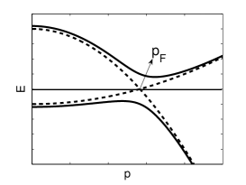
Figure 1: A schematic description of the dispersion relations for the two branches of free fermions (dashed lines) and quasiparticles (solid lines). $p_{F}$ is the common Fermi momentum.

The transition temperature $T_{c}$ is determined by the gap equation at finite temperature and at $\Delta=0$,

$$\frac{-m}{4\pi a_{s}}=\int_{0}^{\infty}dp\frac{p^{2}}{2\pi^{2}}\left(\frac{1-f(\xi_{p}^{a})-f(\xi_{p}^{b})}{2(\epsilon_{p}-\mu)}-\frac{1}{2\epsilon_{p}}\right),$$ (10)

where $f(x)=1/\left(e^{x/T}+1\right)$ is the Fermi-Dirac distribution function. In the case of weak coupling, the number equations can be approximated by the condition $m_{a}\mu_{a}=m_{b}\mu_{b}$ which gives $\xi_{p}^{a}=2(\epsilon_{p}-\mu)/(1+\alpha)$ and $\xi_{p}^{b}=\alpha\xi_{p}^{a}$. With the standard trickfetter , we can reobtain the $\alpha$-dependence of the ratio $T_{c}/\Delta_{0}$ as shown in Eq. (1). For $\alpha=1$, we recover the standard BCS result $T_{c}\simeq 0.57\Delta_{0}$. If $n$ and $a_{s}$ are fixed, we have the relation between the two critical temperatures,

$$T_{c}(m_{a},m_{b})=\sqrt{m_{a}/m_{b}}T_{c}(m_{a},m_{a}),$$ (11)

which means that the critical temperature for the mixed ⁶Li and ⁴⁰K system is about $\sqrt{1/7}$ of the one for the pure ⁶Li system.

We now start to investigate the low energy collective excitation in the superfluid state. The spontaneous symmetry breaking and the associated Goldstone mode in the superfluid state provides an effective field theory approach for the collective excitationweinberg ; nao ; liu . In our case, the particle number is conserved which corresponds to a global $U(1)$ symmetry of the phase transformation,

$$\psi_{i}(x)\rightarrow e^{i\varphi}\psi_{i}(x),\ \ \ \phi(x)\rightarrow e^{2i\varphi}\phi(x)$$ (12)

with an arbitrary and constant phase $\varphi$. The nonzero condensate $\Delta$ of Cooper pairs in the superfluid state spontaneously breaks the $U(1)$ symmetry, and correspondingly, a Goldstone mode which possesses linear dispersion at low energy is expected to appear. The low energy dynamics of the system at low temperature is then dominated by the Goldstone mode. Since all fermions are gapped in our case, the fluctuation of the amplitude of the order parameter at low temperature can be neglected. Therefore, we can write the order parameter field as

$$\phi(x)=\Delta e^{2i\theta(x)}.$$ (13)

Taking the standard approachnao ; liu , we can transform nonperturbatively the fermion fields as follows,

$$\psi_{i}(x)=\tilde{\psi}_{i}(x)e^{i\theta(x)},\ \ \ \psi_{i}^{*}(x)=\tilde{\psi}_{i}^{*}(x)e^{-i\theta(x)}.$$ (14)

The transformation is designed to eliminate the phase fluctuation $\theta(x)$ dependence from the off-diagonal pairing potential terms $(\psi_{a}^{*}\psi_{b}^{*}\phi+c.c.)$ in the Lagrangian. The $\theta(x)$ dependence can appear only in the kinematic terms of the fermion sector, and the Lagrangian density of the system can be expressed as

$${\cal L}=\tilde{\psi}_{i}^{*}\left(-D_{\tau}+\frac{\vec{D}^{2}}{2m_{i}}-\mu_{i}\right)\tilde{\psi}_{i}+(\Delta\tilde{\psi}_{b}\tilde{\psi}_{a}+c.c.)+\frac{\Delta^{2}}{g}$$ (15)

with $D_{\mu}=\partial_{\mu}+i\partial_{\mu}\theta(x)$. Using the Nambu-Gorkov vector, the partition function can be rewritten as

$$Z=\int[d\Psi^{*}][d\Psi][d\theta]e^{\int_{0}^{\beta}d\tau\int d^{3}{\vec{x}}\left(\Psi^{*}{\cal K}[\theta]\Psi+{\Delta^{2}\over g}\right)}$$ (16)

with the kernel ${\cal K}[\theta]$ defined as

$${\cal K}[\theta]=K[\Delta]-\tau_{3}i\partial_{\tau}\theta-\Sigma_{-}(\nabla\theta)^{2}+\Sigma_{+}i\nabla\theta\cdot\nabla,$$ (17)

where the matrices $\Sigma_{\pm}$ are defined as

$$\Sigma_{\pm}=\frac{1}{2}\left(\begin{array}[]{cc}1/m_{a}&0\\ 0&\pm 1/m_{b}\end{array}\right)$$ (18)

Since the fermionic excitations are gapped at all energies below $\Delta$, for collective excitation with energy below $2\Delta$, we can safely integrate out all fermionic degrees of freedom and obtain an effective action for the collective mode only

$$S[\theta]=\int_{0}^{\beta}d\tau\int d^{3}{\bf x}\ \textrm{Tr}\ln{\cal K}[\theta],$$ (19)

where the trace is taken over the fermion momentum, frequency and Nambu-Gorkov vector. We have neglected here a constant which is irrelevant for the following discussions.

The next task is to expand the action in powers of $\theta(x)$. We use the standard derivative expansion. With the two matrices $V_{1}$ and $V_{2}$ defined in the fermion momentum, frequency and Nambu-Gorkov spacenao ,

$$(V_{1})_{k,k^{\prime}} = \frac{1}{\sqrt{\beta V}}(\nu_{n}-\nu_{n^{\prime}})\theta(k-k^{\prime})\tau_{3}$$

$$+ \frac{1}{\sqrt{\beta V}}i({\bf k}+{\bf k^{\prime}})\cdot({\bf k}-{\bf k^{\prime}})\theta(k-k^{\prime})\Sigma_{+}$$

$$(V_{2})_{k,k^{\prime}} = \frac{1}{2\beta V}\sum_{k^{\prime\prime}}({\bf k}-{\bf k^{\prime\prime}})\cdot({\bf k^{\prime\prime}}-{\bf k^{\prime}})$$ (20)

$$\times \theta(k-k^{\prime\prime})\theta(k^{\prime\prime}-k^{\prime})\Sigma_{-},$$

we can expand the effective action to any order of $\theta$. Since we consider only the low energy behavior of the collective mode, we need only the expansion up to the quadratic term,

$$S[\theta]=\textrm{Tr}[{\cal G}V_{2}]+\frac{1}{2}\textrm{Tr}[{\cal G}V_{1}{\cal G}V_{1}].$$ (21)

After a straightforward calculation, we have

$$S[\theta]=\sum_{q}\left[-\frac{{\cal D}(q)}{2}\omega_{n}^{2}+\left({\cal P}(q)+\eta\right)\frac{{\bf q}^{2}}{2}\right]|\theta(q)|^{2}$$ (22)

with the four momentum $q=(i\omega_{n},{\bf q})$ of the collective mode, $\eta=n_{a}/m_{a}+n_{b}/m_{b}$, and

$${\cal D}(q) = \frac{1}{\beta V}\sum_{p}\textrm{Tr}\left[\tau_{3}{\cal G}(p)\tau_{3}{\cal G}(p+q)\right],$$ (23)

$${\cal P}(q) = \frac{1}{\beta V}\sum_{p}\frac{{\bf p}^{2}}{3}\textrm{Tr}\left[\Sigma_{+}{\cal G}\left(p-\frac{q}{2}\right)\Sigma_{+}{\cal G}\left(p+\frac{q}{2}\right)\right].$$

Now the trace is taken only over the Nambu-Gorkov vector. We should note that the functions ${\cal D}$ and ${\cal P}$ are related to the density and current correlation functionsnao ; liu $\langle\rho(x)\rho(0)\rangle$ and $\langle J_{i}(x)J_{j}(0)\rangle$, respectively. Also, we want to emphasize that due to the mass difference, the function ${\cal P}$ is quite different from its usual form in the case with equal masses.

We now discuss the low energy behavior of the collective mode. The energy of the collective mode is defined through the analytical continuation $i\omega_{n}\rightarrow\omega+i0^{+}$. In the low energy limit, namely $\omega\ll 2\Delta$ and $v_{F}|{\bf p}|\ll 2\Delta$, where the Fermi velocity $v_{F}$ is defined as $v_{F}=p_{F}/m$, we can expand the functions ${\cal D}$ and ${\cal P}$ in powers of the momentum ${\bf q}$. To the leading order, the effective action becomes

$$S[\theta] = \frac{1}{2}\sum_{q}\left(A\omega_{n}^{2}+B{\bf q}^{2}\right)|\theta(q)|^{2},$$

$$A = \int_{0}^{\infty}dp\frac{p^{2}}{2\pi^{2}}\frac{\Delta^{2}}{E_{p}^{3}},$$

$$B = \frac{n}{m}-\frac{1}{3}\left(\alpha-1\over\alpha+1\right)^{2}\int_{0}^{\infty}dp\frac{p^{4}}{2\pi^{2}m^{2}}\frac{\Delta^{2}}{E_{p}^{3}}.$$ (24)

Note that the second term of $B$ comes from ${\cal P}(0)$ which vanishes for symmetric systems with $\alpha=1$. The energy spectrum of the collective mode is obtained by finding the zero of the coefficient of the quadratic term in $\theta$,

$$\omega=v_{s}|{\bf q}|$$ (25)

with the definition for the sound velocity $v_{s}=\sqrt{B/A}$. In weak coupling limit, the chemical potentials $\mu_{a}$ and $\mu_{b}$ of the two species are approximately their Fermi energies, and the average chemical potential $\mu$ is much larger than the gap parameter, the integrations in $A$ and $B$ can then be integrated out,

$$A\simeq\frac{mp_{F}}{\pi^{2}},\ \ \ B\simeq\frac{n}{m}-\frac{1}{3}\left(\alpha-1\over\alpha+1\right)^{2}\frac{p_{F}^{3}}{\pi^{2}m}.$$ (26)

Together with the total fermion number $n=p_{F}^{3}/(3\pi^{2})$, the sound velocity has the same mass ratio dependence as the ratio $T_{c}/\Delta_{0}$,

$$v_{s}={v_{F}\over\sqrt{3}}\left({2\sqrt{\alpha}\over 1+\alpha}\right).$$ (27)

In the limit $\alpha\rightarrow 1$, we recover the well known result $v_{s}=v_{F}/\sqrt{3}$. In the other limit $\alpha\rightarrow\infty$, the sound velocity tends to be zero.

At sufficient low temperature $T\ll T_{c}$, the specific heat $c$ is dominated by the Goldstone mode which has the $T^{3}$ power law

$$c=\frac{2\pi^{2}}{15v_{s}^{3}}T^{3},$$ (28)

which means that the specific heat for the mixed ⁶Li and ⁴⁰K system is about 17 times the one for the pure ⁶Li system if $n$ is keep fixed. By experimentally measuring the specific heat, we can determine the sound velocity and check the theoretic result.

If the fermions carry electric charges, the Goldstone mode will disappear due to the long range electromagnetic interaction between the fermionsnao . In the language of gauge field theory, the Goldstone mode is eaten up by the electromagnetic field via Anderson-Higgs mechanism. This phenomenon is also called Meissner effect. Suppose the two species carry charges $eQ_{a}$ and $eQ_{b}$, respectively, the London penetration depth $\lambda_{L}$ is related to the function ${\cal P}$he ,

$$\frac{1}{4\pi\lambda_{L}^{2}}=\frac{ne^{2}}{2m}(Q_{a}^{2}+Q_{b}^{2})+e^{2}{\cal P}(0)$$ (29)

with the modified matrix

$$\Sigma_{+}=\left(\begin{array}[]{cc}Q_{a}/m_{a}&0\\ 0&Q_{b}/m_{b}\end{array}\right)$$ (30)

appeared in ${\cal P}$ due to the charge difference between the two species.

For a neutral Cooper pair with $Q_{a}=-Q_{b}=1$, the inverse of the London penetration depth squared is zero as we expected,

$$\frac{1}{4\pi\lambda_{L}^{2}}=\frac{ne^{2}}{m}-\frac{e^{2}}{3}\int_{0}^{\infty}dp{p^{4}\over 2\pi^{2}m^{2}}{\Delta^{2}\over E_{p}^{3}}=0.$$ (31)

For the case with $Q_{a}=Q_{b}=1$, the mass ratio dependence is again the same as the ratio $T_{c}/\Delta_{0}$ and the sound velocity $v_{s}$,

$$\lambda_{L}^{-1}=\sqrt{4\pi ne^{2}\over m}\left({2\sqrt{\alpha}\over 1+\alpha}\right).$$ (32)

In the limit $\alpha\rightarrow 1$, we recover the familiar penetration depth $\lambda_{L}^{-1}=\left(4\pi ne^{2}/m\right)^{1/2}$. On the other hand, in the limit $\alpha\rightarrow\infty$, the penetration depth approaches infinity, which means an ideal type-II superconductor. Since the penetration depth depends strongly on the mass difference, it may change the type of superconductorstype .

Figure 2: The common $\alpha$ dependence of the ratio of the transition temperature to the zero temperature gap, the sound velocity, and the inverse penetration depth.

For systems with fixed reduced mass $m$ (and hence fixed $v_{F}$) but different mass ratio $\alpha$, from the equations (1), (27) and (32), we can define a quantity $r$ which describes the common mass ratio dependence of $T_{c}/\Delta_{0},v_{s}$ and $\lambda_{L}^{-1}$,

$$r={T_{c}(\alpha)/\Delta_{0}(\alpha)\over T_{c}(1)/\Delta_{0}(1)}={v_{s}(\alpha)\over v_{s}(1)}={\lambda_{L}^{-1}(\alpha)\over\lambda_{L}^{-1}(1)}={2\sqrt{\alpha}\over 1+\alpha},$$ (33)

and plot it as a function of $\alpha$ in Fig.2, where $T_{c}(1),\Delta_{0}(1),v_{s}(1)$ and $\lambda_{L}(1)$ are quantities for the symmetric system with equal masses $m_{a}=m_{b}=m$ and equal chemical potentials $\mu_{a}=\mu_{b}=\mu$.

Based on a general four fermion interaction model, we have derived the sound velocity in a superfluid and the penetration depth in a superconductor for systems where the two species of fermions can possess different masses and chemical potentials but keep the same Fermi surface. We found that the sound velocity and the inverse penetration depth have the same mass ratio dependence as the ratio of the transition temperature to the zero temperature gap. While our result is obtained in weak coupling BCS region, we expect that the qualitative effect will still work in strong coupling systems, such as the mixed atom gas of ⁶Li and ⁴⁰K. In this Letter, we did not consider the Fermi surface mismatch which can induce exotic states such as breached pairing and LOFF states. In these states, there exist gapless fermionic excitations and one can not safely integrate out all fermionic degrees of freedom. When we apply the above effective theory to such gapless states, we will get imaginary sound velocity and penetration depthhe , which have been widely discussed in the study of color superconductivityhuang ; ren .

Acknowledgments: We thank Dr.H.Ren for helpful discussions during the work. The work was supported by the grants NSFC10425810, 10435080 and 10575058.

References

• (1) W.V.Liu and F.Wilczek, Phys. Rev. Lett.90, 047002(2003).
• (2) M.M.Forbes, E.Gubankova, W.V.Liu and F.Wilczek, Phys.Rev.Lett.94, 017001(2005).
• (3) H.Caldas, Phys. Rev. A69, 063602(2004).
• (4) H.Caldas, C.W.Morais, A.L.Mota, Phys.Rev.D72, 045008(2005).
• (5) P.F.Bedaque, H.Caldas and G.Rupak, Phys. Rev. Lett. 91, 247002(2003).
• (6) S.T.Wu and S.Yip, Phys.Rev. A67, 053603(2003); L.He, M.Jin and P.Zhuang, cond-mat/0601147.
• (7) A.L.Fetter and J.D.Walecka, Quantum Theory of Many-Particle Systems, McGraw-Hill, INC. 1971.
• (8) S. Weinberg, The Quantum Theory of Fields II: Modern Applications (Cambridge University Press, Cambridgr, England, 1996), Chap. 19.
• (9) Naoto Nagaosa, Quantum Field Theory in Condensed Matter Physics (Springer, Heidelberg, Germany, 1999).
• (10) W.V.Liu, Phys. Rev. Lett.96, 080401(2006).
• (11) I.Giannakis, D.Hou, M.Huang and H.Ren, cond-mat/0603263.
• (12) L.He, M.Jin and P.Zhuang, Phys.Rev. B73, 024511(2006).
• (13) M.Huang and I.Shovkovy, Phys.Rev. D70, R051501(2004); Phys. Rev. D70, 094030(2004).
• (14) I.Giannakis and H.Ren, Nucl. Phys. B723, 255(2005).