Temperature Dependence of the Conductivity Sum Rule in the Normal State due to Inelastic Scattering

Abstract

We examine the temperature dependence of the optical sum rule in the normal state due to interactions. To be concrete we adopt a weak coupling approach which uses an electron-boson exchange model to describe inelastic scattering of the electrons with a boson, in the Migdal approximation. While a number of recent works attribute the temperature dependence in the normal state to that which arises in a Sommerfeld expansion, we show that in a wide parameter regime this contribution can be quite small. Instead, most of the temperature dependence arises from the zeroth order term in the ‘expansion’, through the temperature dependence of the spectral function, and the interaction parameters contained therein. For low boson frequencies this circumstance causes a linear $T$-dependence in the sum rule. We develop some analytical expressions and understanding of the temperature dependence.

I introduction

In the last few years much attention has been focussed on the anomalous temperature dependence of the optical sum rule basov99 ; molegraaf02 ; santander-syro03 ; homes ; boris ; ortolani ; hwang ; bontemps06 . In particular, in a number of superconductors in the underdoped and optimally doped regime the sum rule exhibits a temperature dependence which is anomalous with respect to that expected from a conventional BCS condensation. The origin of this behaviour has been the subject of a number of theoretical explanations hirsch92 ; hirsch00 ; norman02 ; karakozov02 ; schachinger05 ; marsiglio06 . It is probably fair to say that there is no consensus concerning the origin of the observed anomaly below the superconducting critical temperature, $T_{c}$.

Perhaps equally intriguing is the normal state temperature dependence.knigavko04 ; benfatto05 ; knigavko05 ; toschi05 ; benfatto06 Most often the value of the sum rule is plotted versus $T^{2}$, where $T$ is the absolute temperature, and a linear relationship is observed. molegraaf02 ; santander-syro03 ; ortolani This appears natural as a straightforward Sommerfeld expansion produces a finite temperature correction which is quadratic in temperature. However, several researchers ortolani ; benfatto05 ; toschi05 have noticed that the observed temperature dependence is too strong compared with what one would expect with realistic bandwidths in the cuprate materials (for a quantitative analysis of experimental data in cuprates see Ref. benfatto06, ). Moreover, there are clear deviations from $T^{2}$ dependence, santander-syro03 along with some indications of a linear temperature variation of the spectral weight hwang ; bontemps06 so that one is left with the question: within a Fermi liquid approach, what governs the temperature dependence of the optical sum rule in the normal state?

This is the question we address in this paper. To be concrete we use an exchange boson model (Migdal approximation for phonons), which is a weak-coupling approach. This approach is believed to be applicable to phonons, whose possible relevance to the cuprates has been questioned in the last few years lanzara01 . It is more suspect from a theoretical point of view for magnon exchange; nonetheless we simply adopt the Migdal approximation, with justification provided by some researchers chubukov05 . This type of calculation has also recently been carried out by Karakozov and Maksimov karakozov05 . We reinforce their (and our) main message: a strong temperature dependence of the optical sum rule can arise due to interactions. We examine in further detail the dependence on the various parameters of the model. In particular, we show that the finite width of the band, which is crucial for discussing the sum-rule temperature dependence, introduces new features in the electron self-energy, which are usually overlooked in the infinite-bandwidth approximation. Moreover, we show that the sum-rule temperature dependence cannot be attributed merely to the temperature dependence of the imaginary part of the self energy. Indeed, the real part enters in a critical way.

The outline of the paper is as follows. In the next section we outline the formalism, both on the real and imaginary axes. The former is more appropriate for analytical work, whereas the latter is ideal for numerical work. We show results for a wide variety of parameters, which clearly shows how the temperature dependence can go from quadratic to linear in temperature, depending on the boson frequency scale. We also outline how the Sommerfeld contribution can be determined (even in the presence of interactions). It is small always since we use the Fermi energy as a dominant energy scale. We also show how a large but non-infinite energy scale actually qualitatively changes ‘low energy’ results. In section III we adopt a sequence of approximations to illustrate precisely what is required to achieve qualitative and quantitative agreement with the numerical results. We find that the real part of the single particle self energy is required for a clear understanding of the temperature dependence of the sum rule. Finally, we close with a summary.

II formalism

The ”single band” sum rule maldague77 ; hirsch00 ; norman02 ; benfatto05 can be written

$$\int_{0}^{+\infty}d\nu\mathop{\rm Re}\left[\sigma_{\rm xx}(\nu)\right]={\pi e^{2}\over 4\hbar^{2}}\biggl{\{}\frac{4}{N}\sum_{k}{\partial^{2}\epsilon_{k}\over\partial k_{x}^{2}}n_{k}.\biggr{\}}$$ (1)

where $\epsilon_{k}$ is the tight-binding dispersion and $n_{k}$ is the single spin momentum distribution function. In the case of two dimensions with nearest neighbour hopping only, the quantity in braces is given by the negative of the expectation value of the kinetic energy

$$K(T)=\frac{2}{N}\sum_{k}\epsilon_{k}n_{k}.$$ (2)

We have explored elsewhere that the kinetic energy is a good monitor of the sum rule, even in cases beyond nearest neighbour hopping.benfatto05 ; vandermarel03 Therefore in what follows we will use Eq. (2), as it is much simpler to calculate for a given model than the left-hand-side of Eq. (1).

In general, the momentum distribution function is given by

$$n_{k} = {1\over\beta}\sum_{m=-\infty}^{+\infty}G(k,i\omega_{m})e^{i\omega_{m}0^{+}}=$$ (3)

$$= {1\over 2}+{1\over\beta}\sum_{m=-\infty}^{+\infty}{\rm Re}\ G(k,i\omega_{m}),$$

$$= \int_{-\infty}^{+\infty}d\omega\ f(\omega)A(k,\omega)$$

where $G(k,i\omega_{m})$ is the single electron Matsubara Green function with momentum $k$ and frequency $i\omega_{m}$. The $i\omega_{m}$ are the Fermionic Matsubara frequencies, $i\omega_{m}=\pi T(2m-1)$, where $m$ is an integer, $T$ is the temperature ($k_{B}\equiv 1$), and $\beta\equiv 1/T$ is the inverse temperature. The spectral function, $A(k,\omega)\equiv-{1\over\pi}{\rm Im}G(k,i\omega_{m}\rightarrow\omega+i\delta)$, is related to the analytical continuation of the Matsubara Green function. Finally, $f(\omega)\equiv 1/(e^{\beta\omega}+1)$ is the Fermi-Dirac distribution function. In the absence of interactions the spectral function is a temperature-independent Dirac delta function, so that $n_{k}\equiv f(\epsilon_{k}-\mu)$ and Eq. (2) reduces to:

$$K_{\rm free}(T)=\frac{2}{N}\sum_{k}\epsilon_{k}f(\epsilon_{k}-\mu)$$ (4)

It is then clear that the only temperature dependence of the sum rule (4) can be due to the ”thermal smearing”, i.e. the effect contained within the Fermi-Dirac distribution function. A Sommerfeld expansion then reveals this temperature dependence to be quadratic in $T/W$, vandermarel03 ; benfatto05 where $W$ is the electronic bandwidth; this parameter is usually small at temperatures of interest (up to $200\sim 300$ K). However, in the general case of an interacting system Eq. (2) can be written, by means of Eq. (3), as

$$K(T)=2\int d\epsilon\ d\omega\ N(\epsilon)\epsilon A(\epsilon,\omega)f(\omega)$$ (5)

where we converted the momentum sum to an energy integration in Eq. (2). In the presence of interactions, the Green function $G$ is given by the Dyson equation,

$$G(k,z)=1/\bigl{[}z-\epsilon_{k}-\Sigma(k,z)\bigr{]},$$ (6)

where $z$ is anywhere in the complex plane, and $\Sigma(k,z)$ is the electron self energy. This quantity, and consequently the spectral function $A(\epsilon,\omega)$, will be in general temperature dependent, and it is this temperature dependence that will manifest itself in the total kinetic energy (5)(and therefore the conductivity sum) that we wish to understand.remark1 Indeed, using for simplicity a constant density of states in Eq. (5), an application of the Sommerfeld expansion produces ashcroft76

$$K(T) = K_{0}(T)+K_{somm}(T)=$$ (7)

$$= K_{0}(T)+{\pi^{2}\over 6}(k_{B}T)^{2}{dH(\omega)\over d\omega}|_{\omega=0}$$

where the second term is what we refer to in what follows as the Sommerfeld term (with chemical potential assumed to be zero, in the middle of the band) and

$$H(\omega)={2\over W}\int_{-W/2}^{+W/2}d\epsilon\ \epsilon A(\epsilon,\omega).$$ (8)

In the non-interacting case $H(\omega)$ reduces to $2\omega/W$, so that the $T^{2}/W$ dependence of the Sommerfeld term is recovered, as stated above. In the interacting case instead $dH(\omega)/d\omega$ is affected by the quasiparticle renormalization toschi05 (see Eq. (15) below) and can also bring additional temperature dependence to the $T^{2}$ factor of Eq. (7). The first term $K_{0}(T)$ in Eq. (7) reduces to the constant value $K(T=0)$ in the absence on interactions, see Eq. (4). However, in the general case it is given by

$$K_{0}(T)=\int_{-\infty}^{0}d\omega\ H(\omega)=\int_{-\infty}^{0}d\omega\ {2\over W}\int_{-W/2}^{+W/2}d\epsilon\ \epsilon A(\epsilon,\omega).$$ (9)

The key observation, also made (independently) by Karakozov and Maksimov karakozov05 is that Eq. (9) can have a far more significant temperature dependence than the Sommerfeld contribution. Moreover, as we shall investigate here, due to this effect the temperature dependence of the kinetic energy can deviate from the non-interacting case.

As mentioned in the introduction, this work will focus on “conventional” interactions, modelled after the electron-phonon interaction, as described by an Einstein oscillator with frequency $\omega_{E}$ and coupling strength $\lambda$. In the non-selfconsistent Migdal approximation, the self energy is given by:

$$\Sigma(i\omega_{m})={W\over N\beta}\sum_{k^{\prime},m^{\prime}}\lambda(i\omega_{m^{\prime}}-i\omega_{m})G_{0}(k^{\prime},i\omega_{m^{\prime}}),$$ (10)

where the non-selfconsistency is reflected in the fact that the non-interacting electron Green function is used (hence the subscript zero). This can be made self-consistent but the changes are minor because of the large bandwidth we will always adopt (in other words we are not pursuing the possibility of strong temperature dependence arising from a low electronic energy scale). Here

$$\lambda(z)\equiv{\lambda\omega_{E}^{2}\over\omega_{E}^{2}-z^{2}},$$ (11)

where $z$ is anywhere in the complex plane. The bandwidth $W$ is included in Eq. (10) since it is customary to have a density of states factor in $\lambda$ (which, among other things, makes it dimensionless), and so we use the ‘average’ density of states, $1/W$. One can readily evaluate Eq. (10) for various tight-binding models and use this in Eqs. (6,3,2). However, we simplify further before presenting results and advise the reader that such details make little difference in our conclusions. To this end we assume a constant density of states for energies $-W/2<\epsilon<W/2$. Then the k-summation becomes a single integral over energy, $\epsilon$. The result is

$$\Sigma(i\omega_{m})={\lambda\omega_{E}\over 2}\int_{-W/2}^{+W/2}d\epsilon\ \biggl{(}{N(\omega_{E})+f(\epsilon)\over i\omega_{m}+\omega_{E}-\epsilon}$$

$$+{1+N(\omega_{E})-f(\epsilon)\over i\omega_{m}-\omega_{E}-\epsilon}\biggr{)}$$ (12)

where $N$ and $f$ are the Bose and Fermi functions, respectively. Eq. (12) can be evaluated either at the Matsubara frequencies $i\omega_{m}\equiv i\pi T(2m-1)$, with $m$ an integer, or at the real frequencies attained through direct analytical continuation, $i\omega_{m}\rightarrow\omega+i\delta$, with $i\delta$ an infinitesimal imaginary part. To obtain reliable numerical results the most straightforward approach is on the imaginary axis, as we now describe.

II.1 Imaginary axis formulation

First, one evaluates the integrals in Eq. (12) numerically. One can show that the result is pure imaginary (because of the particle-hole symmetry), and so one can define a “renormalization” function through $\Sigma(i\omega_{m})\equiv i\omega_{m}(1-Z(i\omega_{m}))$, where $Z(i\omega_{m})$ is a real-valued function. Next one returns to the kinetic energy; the momentum dependence (i.e. the $\epsilon$ dependence) in Eq. (2) is simple enough (see the first line of Eq. (3) with $\epsilon$ dependence coming only from the explicit dependence shown in Eq. (6)) to be done analytically. The result is:

$$K(T)=-{4\over\beta}\sum_{m=1}^{\infty}\Biggl{[}1-{\omega_{m}Z(i\omega_{m})\over W/2}{\rm tan}^{-1}\biggl{(}{W/2\over\omega_{m}Z(i\omega_{m})}\biggr{)}\Biggr{]}.$$ (13)

This is easily summed provided asymptotics are used for the contribution at high frequencies. Eq. (13) with $Z(i\omega_{m})$ obtained from Eq. (12) provides us with our numerical results.

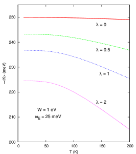
Figure 1: The negative of the kinetic energy vs. temperature for a variety of coupling strengths. Note that the magnitude of the temperature variation increases considerably with coupling strength, and, as explained in the text, this cannot be attributed to the impact of interactions on the Sommerfeld term.

It is difficult to develop an intuition for what temperature dependence may emerge from various parameter choices. In particular we have uncertainty about the energy scale of the boson. Before developing some analytical approximations we therefore show some results. Fig. 1 shows the (negative of the) kinetic energy vs. temperature for several coupling strengths: $\lambda=0,0.5,1$ and $2$ as labeled. We have used a consistent set of parameters for these results: (i) a bandwidth $W=1$ eV, and (ii) a boson frequency $\omega_{E}=25$ meV. The first most noticeable trend is that the absolute value of the kinetic energy decreases with increasing coupling strength. This is expected, as coupling to a boson ’decoheres’ the electrons. While the momentum distribution function retains a discontinuity at the Fermi level (see, for example, Fig. 1 in Ref. marsiglio06, ), the overall distribution is considerably more smeared than in the non-interacting case. Thus, in the ground state, higher kinetic energy (i.e. lower absolute value) states are occupied while low kinetic energy states remain unoccupied. This sort of trend with coupling strength would be very difficult to observe in the experiments, however, as there is no simple way to compare two systems whose only difference is the coupling strength. A more promising property to focus on is the temperature dependence, which clearly varies as the coupling strength increases. Before doing this we wish to make one important remark concerning our parameter choices. Note that the bandwidth has been chosen to be by far the largest energy scale in the problem. This is generally the case in ‘conventional’ metals. Interesting effects can arise when the bandwidth is not so large compared to the other energy scales (such as the boson frequency or the temperature itself) dogan03 ; cappelluti03 . However, here we wish to demonstrate that even in the ‘conventional’ case a significant temperature dependence of the kinetic energy appears due to interactions.

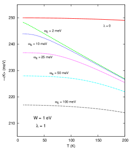
Figure 2: The negative of the kinetic energy vs. temperature for a variety of boson frequencies. Note that with decreasing phonon frequency not only is the magnitude of the temperature variation increased, but it clearly crosses over from quadratic to linear in temperature.

As we explained above, for the non-interacting case the deviation of $K(T)$ from a constant is given by the $T^{2}/W$ Sommerfeld contribution. benfatto05 ; benfatto06 The finite-temperature corrections for the interacting cases shown in Fig. 1 are clearly not simply quadratic, and furthermore the magnitude of the variation increases substantially with coupling strength. Is this due to alterations in the Sommerfeld contribution? The answer is most definitively no. Indeed, even though the Sommerfeld correction (to be further described below) changes by at most $65\%$ (at $200$ K) from $\lambda=0$ to $\lambda=2$, this gives a correction of about $1.7$ meV (at $200$ K) for $\lambda=2$, whereas the deviation from the zero temperature result is $\approx 20$ meV. Thus the bulk of the temperature correction arises from other sources.

How does the energy scale of the Einstein frequency $\omega_{E}$ affect the temperature dependence? In Fig. 2 we show the (negative of the) kinetic energy vs. temperature for several Einstein frequencies with the same bandwidth as before, and with a moderate coupling strength, $\lambda=1$. It is clear that the energy scale of the boson frequency has a profound effect both on the zero temperature value and the temperature dependence itself. In particular, for low boson frequencies the temperature dependence is linear; in addition, as will be made clear below, the temperature dependence comes almost entirely from $K_{0}(T)$, not the Sommerfeld term. In contrast, for high boson frequency the temperature dependence resembles that of the non-interacting case and a significant fraction comes from the Sommerfeld term.

II.2 Real axis formulation: Sommerfeld contribution

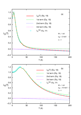
Figure 3: The mass enhancement parameter vs. temperature for (a) $\omega_{E}=2$ meV, and (b) $\omega_{E}=10$ meV. Note the (very) slight deterioration of the approximate result as the boson frequency increases. Also note that for low boson frequency the mass enhancement parameter becomes negative for high temperatures (but ‘high’ being defined relative to the boson, not the electronic energy scale). Counterintuitively, the result for infinite bandwidth (dashed green curve) becomes poorer as the boson energy scale decreases.

To see how this significant temperature variation arises, let us go back to the real-axis formulation (5)-(7) of the kinetic energy and let us analyze the Sommerfeld contribution. To obtain the self energy on the real axis a straightforward analytical continuation of Eq. (12) is required,

$$\Sigma(\omega+i\delta)={\lambda\omega_{E}\over 2}\int_{-W/2}^{+W/2}d\epsilon\ \biggl{(}{N(\omega_{E})+f(\epsilon)\over\omega+i\delta+\omega_{E}-\epsilon}+$$

$${1+N(\omega_{E})-f(\epsilon)\over\omega+i\delta-\omega_{E}-\epsilon}\biggr{)}.$$ (14)

Writing the real and imaginary parts as $\Sigma=\Sigma_{1}+i\Sigma_{2}$, it is easy to see that $\partial\Sigma_{2}(\omega)/\partial\omega$ is zero at zero frequency. Furthermore, $\Sigma_{1}(\omega=0)=0$. Defining, as usual, $\partial\Sigma_{1}(\omega)/\partial\omega|_{\omega=0}\equiv-\lambda_{0}(T)$, then we obtain,

$${\partial A(\epsilon,\omega)\over\partial\omega}|_{\omega=0}=-{2\over\pi}\epsilon(1+\lambda_{0}(T)){\Sigma_{2}(T,\omega=0)\over[\epsilon^{2}+\Sigma_{2}^{2}(T,\omega=0)]^{2}},$$ (15)

Substitution into the second term of Eq. (7) yields, for the Sommerfeld contribution,

$$K_{\rm Somm}={\pi\over 3}(1+\lambda_{0}(T))\biggl{(}{T\over W/2}\biggr{)}^{2}{W\over 2}\times$$

$$\Biggl{(}{\rm tan}^{-1}\biggl{(}{W/2\over|\Sigma_{2}(T)|}\biggr{)}-{{|\Sigma_{2}(T)|\over W/2}\over 1+\bigl{(}{|\Sigma_{2}(T)|\over W/2}\bigr{)}^{2}}\Biggr{)}.$$ (16)

Here, the zero frequency imaginary part of the self energy (denoted simply by $\Sigma_{2}(T)$) is required; for a constant density of states the (exact) result is given by the result known as being a good approximation for the infinite bandwidth case allen82 ,

$$\Sigma_{2}(T)=-\pi\lambda\omega_{E}/{\rm sinh}(\beta\omega_{E}).$$ (17)

At low temperatures this is zero, while at high temperatures (with respect to the boson frequency, $\omega_{E}$), this is linear in temperature.

The real part of the self energy, required to determine $\lambda_{0}(T)$, is more difficult. For $\omega_{E}<W/2$ (the physically relevant case) we obtain

$$\lambda_{0}(T)=\lambda\Biggl{(} 4\pi T\sum_{m=1}^{\infty}{\omega_{m}\omega_{E}^{2}\over[\omega_{m}^{2}+\omega_{E}^{2}]^{2}}\Bigl{[}1-{2\over\pi}{\rm tan}^{-1}\bigl{(}{\omega_{m}\over W/2}\bigr{)}\Bigr{]}$$ (18)

$$-{2\over{\rm sinh}(\beta\omega_{E})}{\omega_{E}\over W/2}{1\over 1-\bigl{(}{\omega_{E}\over W/2}\bigr{)}^{2}}$$

$$+{\omega_{E}\over 2T}f(\omega_{E})[1-f(\omega_{E})]{\rm ln}\Biggl{|}{1+{\omega_{E}\over W/2}\over 1-{\omega_{E}\over W/2}}\Biggr{|}\Biggr{)},$$

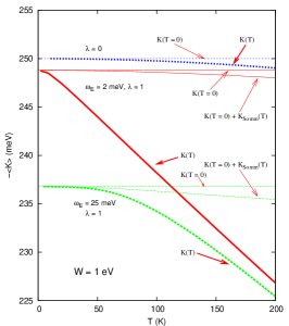
Figure 4: The negative of the kinetic energy vs. temperature showing the breakdown for the various contributions. The solid (red) curves are for small boson frequency, $\omega_{E}=2$ meV, with $\lambda=1$. The two thin lines show how the zero temperature value is modified by the Sommerfeld term by a very small amount; the full numerical result is given by the thick red curve. A similar contribution is found for the non-interacting case (actually, there it is a bit larger) by the dotted (blue) curves. However, here the relative effect is much larger because only the Sommerfeld term is responsible for the temperature variation. Finally, for higher boson frequency, the dashed (green) curves illustrate the amount of temperature variation due to the Sommerfeld term compared with the rest.

where $f(\omega_{E})$ is the Fermi function. This expression is not very enlightening. However note that the first line is strongly convergent, so much so that the ${\rm tan}^{-1}$ term is not really required for most parameter regimes of interest. The Matsubara sum can then be performed, and one obtains for this first term (without the $\lambda$ out front), $-\bar{\omega}_{E}{\rm Im}\psi^{\prime}({1\over 2}+i\bar{\omega}_{E})$, where $\bar{\omega}_{E}=\omega_{E}/(2\pi T)$ and $\psi(z)$ is the diagamma function; this is the result one obtains for the infinite bandwidth case. It is positive definite, starts at unity at zero temperature (so $\lambda_{0}(T\sim 0)\approx\lambda$) and goes to zero as $(\omega_{E}/T)^{2}$ at high temperature. The other two terms vanish for infinite bandwidth. In fact the third term is very small for all temperatures with conventional parameters, while the second term dominates at high temperature. This is clear since it increases (in magnitude) linearly with temperature. A plot is shown in Fig. 3. Also shown is the approximation

$$\lambda^{\rm app}_{0}(t)\sim-\lambda\bar{\omega}_{E}{\rm Im}\psi^{\prime}({1\over 2}+i\bar{\omega}_{E})+{2\over\pi}{\Sigma_{2}(T)\over W/2},$$ (19)

where we have used Eq. (17). This approximation is shown by the symbols and is clearly excellent over the entire temperature range. The important feature apparent in Fig. 3 is that the mass enhancement parameter $\lambda_{0}(T)$ changes sign as the temperature increases. This is a non-trivial effect; Cappelluti et al. cappelluti03 noted a similar phenomenon when impurity scattering was included (we remind the reader that at high temperature low frequency phonons behave much like static impurities). This behaviour is necessary to include to describe the numerical results accurately, as we shall see below. It is truly remarkable that at temperatures below $100$ K a modest scattering ($\lambda=1$) off low frequency phonons ($\omega_{E}=2$ meV) exhibits a qualitative change (mass enhancement changes sign) when an electronic cutoff energy (normally taken to be infinite) is introduced which is 2-3 orders of magnitude larger (1 eV) than the low energy parameters.

Once we have exactly determined the quasiparticle renormalization parameter $\lambda_{0}(T)$ we can estimate the Sommerfeld contribution. The results are plotted in Fig. 4, where we compare again the non-interacting case with the $\lambda=1$ cases at two phonon frequencies. As one can see, in the non-interacting case the Sommerfeld term, even if small, is the only source of the temperature variation of the kinetic energy. When interactions are present instead its contribution cannot account for the temperature variation of $K(T)$ obtained through the numerical computation of Eq. (13). We then conclude that to understand the origin of the strong temperature dependence displayed in Figs. 1-2, one must examine Eq. (9). Note that a different conclusion was instead drawn in Ref. toschi05, , where a Hubbard-like interaction between electrons was considered. Indeed, in this case the main effect of the interaction is to reduce the effective quasiparticle bandwidth $1/\lambda_{0}$, so that as $\lambda_{0}$ increases the Sommerfeld term continues to provide the largest contribution to the temperature variation of the kinetic energy.

III origin of the linear temperature dependence

III.1 Imaginary part of the self energy

The linear temperature dependence, and, indeed, the strongest temperature dependence, occurs for low boson frequency, so we focus on this parameter regime. To put this another way, one should examine temperatures which are high compared to the boson frequency, which Fig. 2 illustrates is readily attained in the $100\sim 200$ K range when $\omega_{E}{<\atop\sim}25$ meV. Then it is clear that the imaginary part of the self energy at zero frequency increases linearly with temperature (see Eq. (17)) and one is tempted to associate the linear temperature dependence observed in $K(T)$ with the linear temperature dependence in $\Sigma_{2}(T)$. In fact, Karakozov and Maksimov karakozov05 noted that the infinite frequency limit of the self energy (as defined by the theory with infinite bandwidth), which we will denote by $\Sigma_{2\infty}(T)$, also increases linearly with temperature, and they use this quantity. It is given by

$$\Sigma_{2\infty}(T)=-\pi{\lambda\omega_{E}\over 2}{\rm coth}\bigl{(}{\beta\omega_{E}\over 2}\bigr{)}.$$ (20)

We should be clear here; the physical self energy always has an imaginary part which goes to zero beyond the electronic bandwidth energy scale. However, the standard theory allen82 ; marsiglio03 eliminates this cutoff, and then Eq. (20) provides the imaginary part of the self energy in the infinite frequency limit.

Either Eq. (20) or (17) provides the correct high temperature behaviour for the imaginary part of the self energy. However, as we now illustrate, using this part of the self energy alone is not sufficient to properly reproduce the numerical result. To examine what the necessary ingredients are, we proceed in steps, and illustrate what approximations to the self energy are sufficient in Eq. (9) to reproduce accurately the numerical result. A first step (following Ref. karakozov05, ) is to model the self energy with a constant pure imaginary part, which we take to be $\Sigma_{2\infty}(T)$. Then the spectral function is given by

$$A(\epsilon,\omega)={1\over\pi}{|\Sigma_{2\infty}(T)|\over(\epsilon-\omega)^{2}+\Sigma_{2\infty}^{2}(T)}$$ (21)

over all frequency, $\omega$. Insertion into Eq. (9) then allows both integrals to be done analytically. If we first assume that Eq. (21) holds for all frequencies ($\omega$), then Eq. (9) results in

$$K_{0a}(T)=-{W\over 4}\Biggl{[}[1+x^{2}]{2\over\pi}{\rm tan}^{-1}({1\over x})-{2\over\pi}x\Biggr{]}.$$ (22)

where $x\equiv{|\Sigma_{2\infty}(T)|\over W/2}$. Clearly, as $|\Sigma_{2\infty(T)}|$ decreases compared with $W/2$, $K_{0}\rightarrow-W/4$, as for the non-interacting case. This result (green, dashed curve), along with the numerical result (solid, red curve), is shown in Fig. 5.

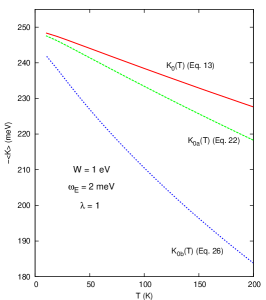
Figure 5: Various approximations of the kinetic energy (without the Sommerfeld expansion terms) compared with the numerical result (solid red curve). The green (dashed) curve is given by Eq. (22), where only the imaginary part of the self energy is included. It is not so far off the numerical result. However, the (relatively small) degree to which a discrepancy exists is serendipitous, as an obvious improvement (introduction of a cutoff - see Fig. 6) results in the blue (dotted) curve. This latter ‘improved’ result is in far worse agreement with the numerics.

Note that the numerical result is that for $K_{0}(T)$; this differs from the results presented in Figs. 1 - 2 by essentially the Sommerfeld term, which we leave out of this discussion. In fact we have checked that a numerical evaluation of $K_{0}(T)$ based on the exact self energies inserted into Eq. (9) agrees with the imaginary axis result with the Sommerfeld term subtracted. The result in Fig. 5 is somewhat disappointing. Clearly, a linear dependence on temperature is obtained, and is easily traced to the linear dependence of $\Sigma_{2\infty}(T)\approx-\pi\lambda T$ for $T>>\omega_{E}$ (note that $\Sigma_{2}(T)$ — see Eq. (17) — has the same high temperature behaviour). Indeed, as $x\ll 1$ in Eq. (22), one finds $K_{0a}(T)\approx K(0)-(2/\pi)\Sigma_{2\infty}(T)$. However, the slope is evidently incorrect, and one may wonder how the discrepancy arises.

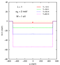
Figure 6: Imaginary part of the self energy for various temperatures. At high temperatures, the use of a constant to describe the imaginary part of the self energy works very well; there is structure at the cutoffs barely visible on the scale shown here, but they are not very important. Despite this accurate analytical representation of the imaginary part of the self energy, this approximation does not work well for the kinetic energy, as explained in Fig. 5.

A possibility presents itself when one examines more closely the imaginary part of the self-energy obtained analytically from Eq. (14) and plotted in Fig. 6. The full expression at positive frequency is:

$$\Sigma_{2}(z) = -\frac{\pi\lambda\omega_{E}}{2}\left[\coth(\beta\omega_{E}/2)+f(z+\omega_{E})-f(z-\omega_{E})\right],$$ (23)

$$\quad z<W/2-\omega_{E},$$

$$\Sigma_{2}(z) = \frac{\pi\lambda\omega_{E}}{2}\left[N(-\omega_{E})+f(z-\omega_{E})\right],$$ (24)

$$\quad W/2-\omega_{E}<z<W/2+\omega_{E},$$

$$\Sigma_{2}(z) = 0,\quad z>W/2+\omega_{E}.$$ (25)

As one can see, except for the small energy range below $z=\omega_{E}$, $\Sigma_{2}$ given by Eq. (23) can be safely approximated by the Eq. (20) above. However, near the band edge $z=W/2-\omega_{E}$ the self energy has a first step-like change to a smaller value, and it then vanishes at $z>W/2+\omega_{E}$. Viewed on the scale of Fig. 6, the fine structure present below $\omega_{E}$ and near the band edges is perhaps not important, while accounting for the upper cutoff $z\approx W/2$ clearly should be. This model can also be solved for analytically. The result is

$$K_{0b}(T)=-{W\over 4} \Biggl{[} [1+x^{2}]{2\over\pi}{\rm tan}^{-1}({1\over x})-{x\over\pi}{\rm ln}\bigl{(}{4+x^{2}\over x^{2}}\bigr{)}$$ (26)

$$- {x^{2}\over\pi}{\rm tan}^{-1}({2\over x})\Biggr{]},$$

where, as before, $x\equiv{|\Sigma_{2\infty}(T)|\over W/2}$. This result is shown in Fig. 5 as the blue dotted curve. Our attempt at improvement has resulted in a significantly inferior approximation!

III.2 Real part of the self energy

One can attempt to improve approximations to the imaginary part of the self energy (for example, by using a proper double step at the band edge), but this does not lead to any improvement in the subsequent $K_{0}(T)$. Success is only attained when the real part of the self energy is included. A clear way to see this is as follows. One first notes that for an approximation which invokes a constant (with frequency) for the imaginary part of the self energy up to the bandwidth (i.e. $\Sigma_{2}(\omega+i\delta)=\Sigma_{2\infty}$ for $|\omega|<W/2$, and zero otherwise), then Kramers-Kronig immediately implies that the real part of the self energy ${\rm Re}\Sigma\equiv\Sigma_{1}$ is given by a simple logarithm, i.e.

$$\Sigma_{1}(\omega+i\delta)={\Sigma_{2\infty}(T)\over\pi}{\rm ln}\Bigl{|}{W/2-\omega\over W/2+\omega}\Bigr{|}.$$ (27)

Then the spectral function can be obtained analytically, and inserted into Eq. (9), with the spectral function given in general by:

$$A(\epsilon,\omega)={1\over\pi}{|\Sigma_{2}(\omega,T)|\over(\epsilon-\omega+\Sigma_{1}(\omega,T))^{2}+\Sigma_{2}^{2}(\omega,T)}.$$

The integral over $\epsilon$ can be performed analytically, but the remaining integral over the frequency, $\omega$, must be done numerically. When this is done, the result for the kinetic energy is essentially indistinguishable from the numerical result at high temperatures.

In light of the ‘failures’ of the approximations in the previous section, this requires further clarification. The ($\omega$) frequency integral in Eq. (9) extends from $-\infty$ to $0$. In the range $-W/2$ to zero the self energy has both a real and imaginary part; then the spectral function is some broad Lorentzian-like function. However, in the range $-\infty<\omega<-W/2$ the imaginary part of the self energy is zero, so the spectral function is given by a delta function. The integral over the variable $\epsilon$ is trivial, and the remaining integral over $\omega$ is non-zero, because the real part in this frequency range is also non-zero. If the real part of the self energy were zero, then this part of the integral (involving the delta function) is also zero, which is why we didn’t mention it earlier with respect to the approximation $K_{0b}(T)$ (see Eq. (26)). Here it must be included, and contributes a significant part (close to $20\%$ of the total).

This discussion firmly establishes the need to include the real part of the self energy in an accurate approximation for the kinetic energy. However, the previous exercise adds little to our fully numerical results, since one of the integrals must be done numerically. To see how well a simplified model does, we adopt the following simpler model. First, we take the imaginary part as before, cut off at $\pm W/2$. For the real part, if one expands Eq. (27) for $|\omega|<<W/2$, the result is

$$\Sigma_{1}(\omega+i\delta)= {2\over\pi}|\Sigma_{2\infty}(T)|{\omega\over W/2}\quad{\rm for}\quad|\omega|<W/2$$

$$= {|\Sigma_{2\infty}(T)|\over\pi}{\rm ln}\Bigl{|}{W/2+\omega\over W/2-\omega}\Bigr{|}\quad{\rm for}\quad|\omega|>W/2.$$

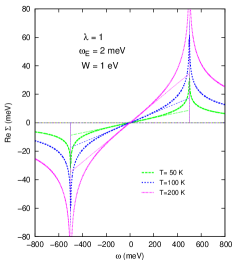
Figure 7: Real part of the self energy for various temperatures. Note that even at the lowest temperature shown (green, dashed curve), the overall slope at the origin looks positive on this scale; in fact there is some structure there, and the slope is in fact negative, but this plays almost no role in our results. This is because the most important contributions to the kinetic energy come from near the bottom of the band. Note that beyond the band edges the approximation given by Eq. (LABEL:real_lin) is indistinguishable from the numerical result on this energy scale (a closer look would reveal some discrepancies — the numerical result has two logarithmic divergences at each band edge at low temperature, not one).

In the first part, we have imposed a cutoff at the band edge. Note that the coefficient of $\omega$ is positive. This always occurs at high temperatures, consistent with the negative mass enhancement displayed in Fig. 4a. In fact, at high temperatures, $|\Sigma_{2\infty}(T)|\approx\pi\lambda T$, and Eq. (LABEL:real_lin) reduces to the second term in Eq. (18), which dominates at high temperature, as Fig. 4 shows. Notice however that while approximation (LABEL:real_lin) holds as soon as $T\gtrsim\omega_{E}/2$ the change in sign in $\lambda_{0}(T)$ occurs at higher temperature. In the second part, we have simply adopted Eq. (27). Fig. 7 shows how accurate this approximation is. In the frequency range $|\omega|<W/2$, the approximation is clearly crude; beyond this frequency range the approximation given by the second half of Eq. (LABEL:real_lin) is indistinguishable from the numerical result. (Actually, if we use Eq. (27), i.e. the logarithm for the entire frequency range, then this would be indistinguishable from the numerical result over the entire frequency range. This accounts for our remarks above that insertion of Eq. (27) along with the constant imaginary part would result in a kinetic energy that is essentially indistinguishable from the full numerical result.)

Explicitly, Eq. (9) becomes

$$K_{0c}(T)={2\over W}\int_{-\infty}^{-W/2}d\omega\int_{-W/2}^{+W/2}d\epsilon\ \epsilon\delta[\omega-\epsilon-\Sigma_{1}(\omega+i\delta)]+$$

$${2\over W}\int_{-W/2}^{0}d\omega\int_{-W/2}^{+W/2}d\epsilon\ \epsilon{1\over\pi}{|\Sigma_{2\infty}(T)|\over(\epsilon-\omega+\Sigma_{1}(\omega+i\delta))^{2}+\Sigma_{2\infty}^{2}(T)}.$$

(29)

In the first line, the $\epsilon$ integration is trivial. Care must be taken concerning the bandedge cutoffs, so that the $\omega$ integration no longer extends to $-\infty$. This lower cutoff, $\omega_{c}$, is determined by the condition $\omega_{c}-{|\Sigma_{2\infty}(T)|\over\pi}{\rm ln}\Bigl{|}{W/2+\omega_{c}\over W/2-\omega_{c}}\Bigr{|}=-W/2$, which can easily be solved by a few iterations. The remaining $\omega$ integral is elementary; we write it as $K_{0c}^{1}(T)$:

$$K_{0c}^{1}(T)=-{W\over 4}\biggl{[}y^{2}-1+{2\over\pi}x\Bigl{[}{\rm ln}\bigl{(}{4\over y^{2}-1}\bigr{)}-y{\rm ln}\bigl{(}{y+1\over y-1}\bigr{)}\Bigr{]}\biggr{]},$$ (30)

where $x$ is as before, and $y\equiv{|\omega_{c}|\over W/2}$. The ratio $y$ is always greater than unity.

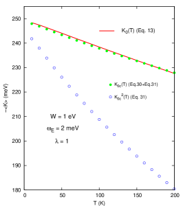
Figure 8: Comparison of $K_{0c}(T)$ approximation (solid green circles) with numerical results (solid red curve). Agreement is excellent. Also shown are the results for $K_{0c}^{2}(T)$ alone, i.e. without accounting for the delta-function part. Clearly both real and imaginary parts of the self energy are necessary for accurate results.

In the second line we write $\Sigma_{1}=-\tilde{\lambda}\omega$, where $\tilde{\lambda}=-{2\over\pi}x$ represents a negative mass enhancement. Substitution into the integral allows this piece (which we denote $K_{0c}^{2}(T)$) to be evaluated analytically as before:

$$K_{0c}^{2}(T)=-{W\over 4}{1\over 1+\tilde{\lambda}}\Biggl{[}(1+x^{2}){2\over\pi}{\rm tan}^{-1}\bigl{(}{1\over x}\bigr{)}$$

$$- {x\over\pi}(1+\tilde{\lambda}){\rm ln}\Bigl{(}{(2+\tilde{\lambda})^{2}+x^{2}\over\tilde{\lambda}^{2}+x^{2}}\Bigr{)}$$

$$+ \Bigl{(}\tilde{\lambda}(\tilde{\lambda}+2)-x^{2}\Bigr{)}{1\over\pi}\Bigl{(}{\rm tan}^{-1}\bigl{(}{2+\tilde{\lambda}\over x}\bigr{)}-{\rm tan}^{-1}\bigl{(}{\tilde{\lambda}\over x}\bigr{)}\Bigr{)}\Biggr{]},$$

with $x\equiv{|\Sigma_{2\infty}(T)|\over W/2}$. The approximation $K_{0c}(T)$ consists of the sum of these two pieces, $K_{0c}(T)=K_{0c}^{1}(T)+K_{0c}^{2}(T)$. These are plotted for $\omega_{E}=2$ meV and $\lambda=1$ in Fig. 8 (solid green circles). Agreement with the numerical result (solid red curve) is now excellent, especially when one considers the crudeness of the approximation for the real part of the self energy shown in Fig. 7. We also show the result for $K_{0c}^{2}(T)$, i.e. without the correction from the delta-function piece (which arises only because the real part of the self energy is non-zero) with the open blue circles. Clearly both real and imaginary parts of the self energy are required for accurate results.

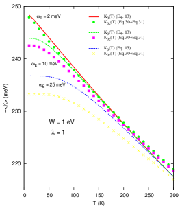
Figure 9: Comparison of analytical model ($K_{0c}(T)$) (symbols) with numerical results (curves) for several boson frequencies. Not the expanded vertical scale. Clearly, the model deteriorates as the boson frequency increases (also note that the result is also no longer linear). Nonetheless, the discrepancy for $\omega_{E}=25$ meV is still less than $2\%$.

Finally, we show results in Fig. 9 for several boson frequencies, over a somewhat higher temperature range. The approximations used to obtain $K_{0c}(T)$ clearly deteriorate as the boson frequency increases with respect to the temperature scale involved. Note in particular that in the temperature regime where the result is no longer linear in temperature the qualitative agreement is not so good (i.e. off by more than a percent). It is also apparent in this figure that the crude approximation for the real part of the self energy (first part of Eq. (LABEL:real_lin)) results in some minor discrepancies at higher temperatures. As mentioned before, replacement of this linear approximation with a single logarithm (still an approximate result) makes the ‘analytic’ results agree essentially perfectly with the numerical results.

IV discussion and summary

In the previous sections we have described the effects of the interaction of electrons with a soft collective mode on the electronic kinetic energy, which is in turn related to the optical sum rule probed by the experiments. In contrast to the general expectation for Fermi-liquid systems, here the main contribution to the temperature variation of the kinetic energy cannot be attributed to the Sommerfeld term, i.e. to the thermal smearing of the Fermi occupation number. Instead, the relevant effects come from the temperature dependence set by the interaction itself, via the electronic self energy. While discussing the sum rule behavior the presence of a finite bandwidth $W$ is a crucial ingredient, since the temperature variations are expected to vary as a power of $T/W$ or $\Sigma_{2}/W$. The latter case is relevant here, with the kinetic energy, as given by Eq.s (30)-(LABEL:koc2), scaling as $\Sigma_{2}/W$. Moreover, since $\Sigma_{2}(T)=-\pi\lambda T$ at high temperatures, we also found a linear temperature depletion of the optical sum. However, in deriving this result we had to properly take into account also the structure of the real part of the self energy, whose behavior at low frequency is quite strongly affected by the presence of a finite-bandwidth cut-off, in contrast to the general expectation coming from the analysis of the infinite-bandwidth approximation.allen82 ; marsiglio03

Finally, we would like to present a simple argument which can help the reader to understand the difference between the effect of thermal smearing of the Fermi function with respect to the effect of the interaction considered here. Going back to the expression (2) of the kinetic energy, we can understand the Sommerfeld term as due to the fact that by varying the temperature one has a variation of the occupation factor $\delta n(\xi)$ of order $\xi/T$ over a range $\sim T$ around the Fermi level (here $\xi=\epsilon-\mu$) and $0$ otherwise so that:

$$\delta K\sim\frac{1}{W}\int_{-T}^{T}d\xi\,(\xi+\mu)\,\delta n(\xi)\sim\frac{T^{2}}{W}=W\left(\frac{T}{W}\right)^{2}.$$ (32)

As a consequence, the $T^{2}$ power is due to the fact that the integration of energy, which gives $\epsilon^{2}$, on a range $T/W$, produces a power of $(T/W)^{2}$ in the kinetic energy. The question then arises: do interactions similarly simply change the occupation number in a region $|\Sigma_{2}|/W$ around the Fermi level, which would then lead to a $(|\Sigma_{2}|/W)^{2}$ dependence of the kinetic energy for the interacting case? The answer we have found is clearly, no. Indeed, when the occupation number coming from Eq. (3) is considered, using the same approximations (20) and (LABEL:real_lin) considered above for the self-energy we can estimate $n_{0}(\epsilon)$ (i.e. the contribution coming from the $T=0$ limit of the Fermi function, in analogy with the definition (9) of $K_{0}(T)$) as:

$$n_{0}(\epsilon)=\frac{1}{\pi(1+\tilde{\lambda})}\left[\tan^{-1}\frac{W(1+\tilde{\lambda})/2+\epsilon}{|\Sigma_{2\infty}|}-\tan^{-1}\frac{\epsilon}{|\Sigma_{2\infty}|}\right],$$ (33)

As a consequence, one can roughly say that $n_{0}(\epsilon)\sim 1-\alpha{|\Sigma_{2\infty}|}/W$, with some coefficient $\alpha$ of order 1, in most of the energy range between $-W/2$ and $0$, and not only in a small region around the Fermi level. In other words, the interaction affects the occupation number even far from the Fermi level, so that the energy integration in Eq. (2) is now scaling as:

$$\delta K\sim\frac{1}{W}\int_{-W/2}^{\mu}d\epsilon\,\epsilon\,\alpha\frac{|\Sigma_{2\infty}|}{W/2}\sim\alpha W\left(\frac{|\Sigma_{2\infty}|}{W}\right).$$ (34)

Thus, the kinetic energy is directly proportional to the temperature variation of the imaginary part of the self energy, even though the exact coefficient $\alpha$ should be determined taking care also of contributions from the real part of the self-energy. Even though the previous relation is not valid for stronger interactions (as in Hubbard-like models toschi05 ), one can reasonably expect that by modeling the inelastic scattering with a more general phonon-like spectrum, the sum rule behavior will roughly follow the modification introduced in the electronic self-energy in the way indicated by Eq. (34). This possibility leads to an understanding of the experimental observation of a non-quadratic temperature dependence of the sum rule in some cuprate superconductors, where also the high-energy scattering rate shows a linear temperature scaling hwang ; bontemps06 .

- (1) D.N. Basov, S.I. Woods, A.S. Katz, E.J. Singley, R.C. Dynes, M. Xu, D.G. Hinks, C.C. Homes, and M. Strongin, Science 283, 49 (1999); A.S. Katz, S.I. Woods, E.J. Singley, T. W. Li, M. Xu, D.G. Hinks, R.C. Dynes and D.N. Basov, Phys. Rev. B61, 5930 (2000).
- (2) H.J.A. Molegraaf, C. Presura, D. van der Marel, P.H. Kes, and M. Li, Science 295, 2239 (2002).
- (3) A.F. Santander-Syro, R.P.S.M. Lobo, N. Bontemps, Z. Konstantinovic, Z.Z. Li, H. Raffy, Europhys. Lett. 62, 568 (2003); A.F. Santander-Syro, R.P.S.M. Lobo, N. Bontemps, W. Lopera, D. Girata, Z. Konstantinovic, Z.Z. Li, H. Raffy, Phys. Rev. B 70, 134504 (2004). G. Deutscher, A.F. Santander-Syro, N. Bontemps, Phys. Rev. B 72, 092504 (2005).
- (4) C.C. Homes, S.V. Dordevic, D.A. Bonn, R. Liang, W.N. Hardy, Phys. Rev. B 69, 024514 (2004).
- (5) A.V. Boris, N.N. Kovaleva, O.V. Dolgov, T. Holden, C.T. Lin, B. Keimer, C. Bernhard, Science 304, 708 (2004).
- (6) M. Ortolani, P. Calvani, S. Lupi, Phys. Rev. Lett. 94, 067002 (2005).
- (7) J. Hwang, J. Yang, T. Timusk, S. G. Sharapov, J. P. Carbotte, D. A. Bonn, Ruixing Liang, and W. N. Hardy, Phys. Rev. B73, 014508 (2006).
- (8) N. Bontemps, R.P.S.M. Lobo, A.F. Santander-Syro, and A. Zimmers, cond-mat/0603024.
- (9) J.E. Hirsch, Physica C 199, 305 (1992); Physica C 201, 347 (1992).
- (10) J.E. Hirsch and F. Marsiglio, Physica C 331, 150 (2000); J.E. Hirsch and F. Marsiglio, Phys. Rev. B62, 15131 (2000).
- (11) M.R. Norman and C. Pépin, Phys. Rev. B 66, 100506 (2002).
- (12) A.E. Karakozov, E.G. Maksimov, and O.V. Dolgov, Solid State Commun. 124, 119 (2002).
- (13) E. Schachinger and J. P. Carbotte, Phys. Rev. B 72, 014535 (2005).
- (14) F. Marsiglio, Phys. Rev. B 73, 064507 (2006).
- (15) A. Knigavko, J. P. Carbotte, and F. Marsiglio, Phys. Rev. B 70, 224501 (2004); Europhysics Letts. 71, 776 (2005).
- (16) L. Benfatto, S. Sharapov, and H. Beck, Eur. Phys. J. B 39, 469 (2004); L. Benfatto, S. G. Sharapov, N. Andrenacci, and H. Beck, Phys. Rev. B 71, 104511 (2005).
- (17) A. Knigavko and J.P. Carbotte, Phys. Rev. B 72, 035125 (2005); cond-mat/0602681, to be published in Physical Review B.
- (18) Th. A. Maier, M. Jarrell, A. Macridin, and C. Slezak, Phys. Rev. Lett. 92, 027005 (2004).
- (19) A. Toschi, M. Capone, M. Ortolani, P. Calvani, S. Lupi, and C. Castellani Phys. Rev. Lett. 95, 097002 (2005).
- (20) K. Haule and G. Kotliar, cond-mat/0601478.
- (21) L. Benfatto and S. Sharapov, cond-mat/0508695, to appear in J. Low Temp. Phys. (2006).
- (22) D. van der Marel, H.J.A. Molegraaf, C. Presura, and I. Santoso, in Concepts in Electron Correlations, edited by A. Hewson and V. Zlatic (Kluwer, 2003). See also cond-mat/0302169.
- (23) A. Lanzara, P.V. Bogdanov, X.J. Zhou, S.A. Kellar, D.L. Feng, E.D. Lu, T. Yoshida, H. Eisaki, A. Fujimori, K. Kishio, J.-I. Shimoyama, T. Noda, S. Uchida, Z. Hussain, and Z.-X. Shen, Nature (London) 412, 510 (2001).
- (24) See, for example, A. V. Chubukov and J. Schmalian, Phys. Rev. B 72, 174520 (2005).
- (25) A.E. Karakozov and E.G. Maksimov, cond-mat/0511185.
- (26) P.F. Maldague, Phys. Rev. B16, 2437 (1977).
- (27) We have previously discussed possible temperature dependence arising from band edge effects benfatto05 ; marsiglio06 . In what follows here we will assume particle-hole symmetry, so that there is no ”extra” temperature dependence arising from these effects.
- (28) N.W. Ashcroft and N.D. Mermin, In: Solid State Physics (Saunders College Publishing, New York 1976)p. 518.
- (29) F. Dogan and F. Marsiglio, Phys. Rev. B 68, 165102 (2003).
- (30) E. Cappelluti and L. Pietronero, Phys. Rev. B 68, 224511 (2003).
- (31) P.B. Allen and B. Mitrović, In: Solid State Physics, edited by H. Ehrenreich, F. Seitz, and D. Turnbull (Academic, New York, 1982) Vol. 37, p.1.
- (32) F. Marsiglio and J.P. Carbotte, Review Chapter in ‘The Physics of Conventional and Unconventional Superconductors’ edited by K.H. Bennemann and J.B. Ketterson (Springer-Verlag), pp. 233-345 (2003). See also cond-mat/0106143.