Incomplete equilibrium in long-range interacting systems

Abstract

We use a Hamiltonian dynamics to discuss the statistical mechanics of long-lasting quasi-stationary states particularly relevant for long-range interacting systems. Despite the presence of an anomalous single-particle velocity distribution, we find that the Central Limit Theorem implies the Boltzmann expression in Gibbs’ $\Gamma$-space. We identify the nonequilibrium sub-manifold of $\Gamma$-space characterizing the anomalous behavior and show that by restricting the Boltzmann-Gibbs approach to this sub-manifold we obtain the statistical mechanics of the quasi-stationary states.

In comparison with its equilibrium counterpart, nonequilibrium statistical mechanics does not rely on universal notions, like the ensembles ones, through which one can handle large classes of physical systems maes . Incomplete (or partial) equilibrium states landau ; incomplete are in this respect a remarkable exception, since in these cases concepts of equilibrium statistical mechanics can be used to describe nonequilibrium situations. Incomplete equilibrium states arise when different parts of the system themselves reach a state of equilibrium long before they equilibrate with each other landau . The classical understanding on how a system approaches equilibrium is based on the short time-scale collisions mechanism which links any initial condition to the statistical equilibrium. For long-range interacting systems, this picture is not valid anymore since the time-scale for microscopic collisions diverges with the range of the interactions. This implies that the Boltzmann equation must be substituted with other approximations such as the Vlasov or the Balescu-Lenard equations balescu , where the interparticle correlations are negligible or almost negligible and a nonequilibrium initial configuration could stay frozen or almost frozen for a very long time. This applies, e.g., to gravitational systems, Bose-Einstein condensates and plasma physics dauxois . Due to the physical relevance of long-range interacting systems and to the privileged position of incomplete equilibrium states in nonequilibrium statistical mechanics, it is important to investigate whether the notion of incomplete equilibrium plays an important role in understanding the nonequilibrium properties of these systems.

Recently we showed ham_can that nonequilibrium states in which the value of macroscopic quantities remains stationary or quasi-stationary for reasonably long time (quasi-stationary states – QSSs) are important, e.g., for experiments, since they appear even when the long-range system exchanges energy with a thermal bath (TB). Using the same paradigmatic long-range interacting system of Ref. ham_can , the Hamiltonian Mean Field (HMF) model konishi , here we discuss the Gibbs’ $\Gamma$-space statistical mechanics description of the QSSs in a canonical ensemble perspective. We identify the nonequilibrium sub-manifold of $\Gamma$-space within which the quasi-stationary dynamics is confined and we show that the Boltzmann-Gibbs (BG) approach, restricted to this sub-manifold, gives the correct statistics of the QSSs. In this respect, the QSSs can be interpreted as incomplete equilibrium states landau . Our theoretical framework allows one to calculate, on the basis of the empirical detection of the temperature and of the value of an order parameter, any other thermodynamic quantity such as the energy or the specific heat of the system. The possibility of predicting physical quantities which characterize the QSSs could be useful, i.e., for understanding nonequilibrium features of gravitational or plasma structures and it is then of particular interest for experimentalists or theorists of long-range interacting systems. Since the system considered is naturally endowed with a microscopic Hamiltonian dynamics, we validate step by step our theoretical derivation with a priori results obtained from dynamical simulations. Our findings also furnish novel significant arguments to an intense debate in the literature latora ; debate_1 ; debate_2 ; debate_3 , that so far has been restricted to the single-particle $\mu$-space and to the microcanonical ensemble.

The HMF model can be introduced as a set of $M$ globally coupled $XY$-spins with Hamiltonian konishi

$$H_{\rm HMF}=\sum_{i=1}^{M}\frac{l_{i}^{2}}{2}+\frac{1}{2M}\sum_{i,j=1}^{M}\left[1-\cos(\theta_{i}-\theta_{j})\right],$$ (1)

where $\theta_{i}\in[0,2\pi)$ are the spin angles and $l_{i}\in\mathbb{R}$ their angular momenta (velocities). The specific magnetization of the system is $m_{\rm HMF}\equiv|\sum_{i=1}^{M}(\cos\theta_{i},\sin\theta_{i})|/M$ and the temperature $T$ is identified with twice the specific kinetic energy. We have thus $e_{\rm HMF}=T_{\rm HMF}/2+(1-m_{\rm HMF}^{2})/2$, where $e_{\rm HMF}\equiv E_{\rm HMF}/M$ is the specific energy. Direct connections with the problem of disk galaxies chavanis and free electron lasers experiments barre have been established for this Hamiltonian. Eq. (1) has also been shown to be representative of the class of Hamiltonians on a one-dimensional lattice in which the potential is proportional to $\sum_{i,j=1}^{M}\left[1-\cos(\theta_{i}-\theta_{j})\right]/r_{ij}^{\alpha}$, where $r_{ij}$ is the lattice separation between spins and $\alpha<1$ tamarit . Hence, the Hamiltonian in Eq. (1) can be considered as an interesting “paradigm” for long-range interacting systems chavanis . The TB introduced in ham_can is characterized by $N\gg M$ equivalent spins first-neighbors coupled along a chain

$$H_{\rm TB}=\sum_{i=M+1}^{N}\frac{l_{i}^{2}}{2}+\sum_{i=M+1}^{N}\left[1-\cos(\theta_{i+1}-\theta_{i})\right],$$ (2)

with $\theta_{N+1}\equiv\theta_{M+1}$, and the interaction between HMF and TB is given by

$$H_{\rm I}=\epsilon\sum_{i=1}^{M}\sum_{s=1}^{S}\left[1-\cos(\theta_{i}-\theta_{r_{s}(i)})\right],$$ (3)

where $\epsilon$ is a coupling constant that modulates the interaction strength between HMF and TB. Each HMF-spin is thus in contact with $S$ TB-spins specified as initial condition ($r_{s}(i)$ are independent integer random numbers in the interval $[M+1,N]$). A “surface-like effect” $S\sim M^{\gamma-1}$ ($0<\gamma<1$) guarantees a consistent thermodynamic limit ham_can . For $\epsilon=0$ HMF and TB are decoupled and the setup reproduces the microcanonical dynamics. For $\epsilon\neq 0$ the whole system is at constant energy whereas the energy of the HMF model fluctuates. Our numerics are obtained with $M=10^{3}$, $N=M^{2}$, $S=10^{5}M^{-1/2}$, $0.005\leq\epsilon\leq 0.1$ (we use dimensionless units), through a velocity-Verlet algorithm assuring a total energy conservation within an error $\Delta E/E<10^{-5}$ ham_can . The width $T_{0}$ of the Maxwellian probability density function (PDF) for the initial TB-velocities is a control parameter for the bath temperature. For $\epsilon>0$ we showed ham_can that the HMF temperature finally converges to the BG equilibrium at temperature $T_{0}$.

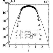
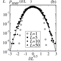
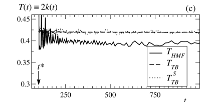
Figure 1: QSS for $M=10^{3}$ and $T_{0}=0.38$. For $\epsilon=0.005$ we observe the average values $m_{\rm HMF}^{2}\simeq 0.015$ and $T_{\rm HMF}\simeq 0.397$ ($e_{\rm HMF}\simeq 0.691$). (a): Single particle velocity PDF. The solid line is $p_{\rm TB}(l)$. (b): PDF of the sum of the velocities of $L$ particles. By multiplying the PDFs for different $L$’s by $L^{0.5}$ and dividing the velocities $l$ by $L^{0.5}$, all data collapse fairly well on to the line that corresponds to a Gaussian distribution with width $T=0.397$. (c): Temperature time-evolutions for three different subsets of the system during the QSSs. Here the TB temperature has been shifted to $T_{0}=0.42$.

By setting far-from-equilibrium initial conditions for the HMF model, the relaxation to equilibrium typically displays stationary or quasi-stationary stages during which the phase functions $m_{\rm HMF}$, $T_{\rm HMF}$ (and thus also $e_{\rm HMF}$) fluctuate around constant or almost constant average values ham_can . This behavior is particularly interesting when the life-time of the QSS diverges in the thermodynamic limit ham_can ; latora ; debate_1 ; debate_2 ; debate_3 . This happens if for example at $t=0$ we set a delta distribution for the angles ($p_{\rm HMF}(\theta)=\delta(0)\Rightarrow m_{\rm HMF}^{2}=1$), a uniform distribution for the velocities, $p_{\rm HMF}(l)=1/2\bar{l},\;l\in[-\bar{l},\bar{l}]$, with $\bar{l}\simeq 2.03$ ($e_{\rm HMF}\simeq 0.69$) ham_can , and a TB temperature $T_{0}=0.38$. In Fig. 1a we show that during the QSS, for $\epsilon>0$, the single particle velocity PDF is non-Maxwellian and similar to the distribution found in the microcanonical case latora ; debate_1 ; debate_2 ($\epsilon=0$).

Given some probability distribution for the initial data, a dynamical estimation of phase functions, like e.g. the energy $E_{\rm HMF}$, can be obtained by recording the phase function values at different times in a single orbit and averaging over different realizations of the initial conditions. To understand the connection between the anomalous PDF in $\mu$-space and the $\Gamma$-space statistics, we start by measuring the PDF of the sum of the velocities of $L$ particles, $p_{\rm HMF}^{L}$ (Fig. 1b). Such a distribution tends very quickly to the Gaussian form as $L$ increases. In fact, a rescaling of $l$ by $L^{1/2}$ and a multiplication of $p_{\rm HMF}^{L}(l)$ by the same factor reveal the Central Limit Theorem (CLT) data collapse onto the Maxwellian (Gaussian) distribution of temperature $T=T_{\rm HMF}=0.397$. The fact that the CLT applies to the sum of the velocities is a strong indication kinchin that in $\Gamma$-space the probability for the energy $E_{\rm HMF}$ is characterized by the Boltzmann expression $\omega(E_{\rm HMF})e^{-E_{\rm HMF}/T}$ ($k_{B}\equiv 1$), where $\omega(E_{\rm HMF})$ is a density of states. Although this situation resembles equilibrium, there are some important differences. For example, the anomalous velocity PDF in $\mu$-space implies that the joint probability of all particles is not given by a mere product of exponentials. The Boltzmann expression arises, because of weak enough particle-particle correlations balescu , for a sufficiently large number of particles. Below, we directly verify its occurrence.

Another key observation is that during the QSS the HMF does not thermalize with the TB. In Fig. 1c we shifted the TB temperature by $10\%$, setting it to $T_{0}=0.42$. While this modifies the final HMF equilibrium temperature, it does not affect $T_{\rm HMF}$ during the QSS. Even the subset of $S$ TB-spins in direct contact with the HMF model, $\{\theta_{r_{s}(i)}\}_{1\leq s\leq S,1\leq i\leq M}$, is at $T_{\rm TB}^{S}=T_{0}$ and does not thermalize with the HMF temperature. The energy fluctuations are nevertheless significantly larger than those due to the algorithm precision ($\Delta E_{\rm HMF}/E_{\rm HMF}\simeq 10^{-2}$ for $M=10^{3}$), distinguishing the canonical QSSs from the microcanonical ones.

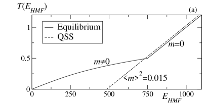
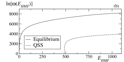
Figure 2: (a): Caloric curve of the HMF model for $M=10^{3}$. Solid line is the BG equilibrium and dashed line is the curve at fixed $m^{2}=0.015$. (b) Theoretical calculation of $\ln[\omega(E_{\rm HMF})]$ by using Eq. (4) with the equilibrium caloric curve (solid line) and with the curve at $m^{2}=0.015$ (dashed line).

We now address the main result of the paper, which is central to the discussion of the appropriate statistical mechanics approach for quasi-stationary nonequilibrium states in long-range systems and to the debate in latora ; debate_1 ; debate_2 ; debate_3 . According to BG, the equilibrium PDF of the energy $E$ for a system in contact with a TB at temperature $T$ is $p_{\rm BG}(E)=\omega(E)e^{-E/T}/Z$, where $Z$ is the partition function. Since the Hamiltonian simulations consent an empirical estimation of this PDF, it is possible to verify $p_{\rm BG}(E)$ on dynamical basis baldovin . From the analytically known solution of the HMF model konishi ; chavanis one obtains the BG equilibrium caloric curve of the system $T(E)$ (full line in Fig. 2a). The integration of the thermodynamic relation $\partial\ln\omega(E)/\partial E=1/T(E)$,

$$\ln[\omega(E)]-\ln[\omega(E_{0})]=\int_{E_{0}}^{E}dE^{\prime}\;\frac{1}{T(E^{\prime})},$$ (4)

furnishes an analytical evaluation of $\omega(E)$ (full line in Fig. 2b) and hence of $p_{\rm BG}(E)$ baldovin . In Fig. 3a we show that, as expected, $p_{\rm BG}(E_{\rm HMF})$ and the result of the simulations at equilibrium, $p(E_{\rm HMF})$, do coincide. A linear regression of $\ln[p(E_{\rm HMF})/\omega(E_{\rm HMF})]$ vs $E_{\rm HMF}$ with a coefficient $R=-0.99997$ gives a direct evidence of the Boltzmann factor (Fig. 3b). Moreover, the inverse of the slope coefficient agrees with the dynamical $T=2k_{\rm HMF}$ within an error $\Delta T/T=0.3\%$.

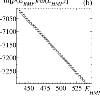
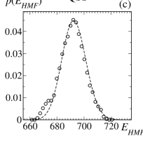
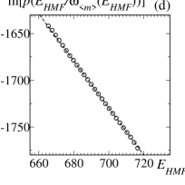
Figure 3: For $N=10^{6}$, $M=10^{3}$ and $\epsilon=0.005$ comparison between the dynamically recorded $p(E_{\rm HMF})$ (empty circles) and $p_{\rm BG}(E_{\rm HMF})$ (dashed lines).

With respect to the QSS, it is interesting to ask latora ; debate_1 ; debate_2 ; debate_3 if there exist a statistical mechanics approach that, equivalently to the BG equilibrium one, can reproduce the dynamically observed $p(E_{\rm HMF})$. We first notice that the anomalous dynamical behavior during the QSS is due to the fact that the system, instead of exploring the overwhelming majority of $\Gamma$-space microstates, is trapped mackay in regions characterized by almost constant nonequilibrium values of the order parameter $m$. Let $\langle m\rangle$ be the average value around which $m$ fluctuates and $\omega_{\langle m\rangle}(E)$ the sub-manifold of $\Gamma$-space which corresponds to this dynamical behavior. The assumption of weak correlations among particles, consistent with the previous argument based on the CLT and with the Vlasov and Balescu-Lenard kinetic pictures balescu , suggests that the Lebesgue measure of $\omega_{\langle m\rangle}(E)$ is non-zero. We then expect $p(E)=p_{{\rm BG},\langle m\rangle}(E)\equiv\omega_{\langle m\rangle}(E)e^{-E/T}/Z$ kinchin . Having assumed this, a saddle point calculation at fixed $m=\langle m\rangle$ (large deviation formulation of the canonical ensemble ellis at $m=\langle m\rangle$) implies that $T$ in the previous expression satisfies the fundamental thermodynamic relation $\partial\ln\omega_{\langle m\rangle}(E)/\partial E|_{E=\langle E\rangle}=1/T$, where $\langle E\rangle$ is the average value of the energy during the QSS. Hence, $\omega_{\langle m\rangle}(E)$ can be calculated by replacing the equilibrium caloric curve $T(E)$ with the caloric curve at constant $m=\langle m\rangle$, $T_{\langle m\rangle}(E)$, and by performing the approach of Eq. (4). The validity of this strategy, and in particular of Eq. (4) for the QSS, is further established by the comparison with the dynamical simulations results. Specifically, we show below that $T$ corresponds to twice the specific kinetic energy of the HMF.

The HMF caloric curve at fixed $m_{\rm HMF}=\langle m_{\rm HMF}\rangle$ is given, for all $\langle m_{\rm HMF}\rangle\in[0,1]$, by the straight line

$$T_{{\rm HMF},\langle m\rangle}(E_{\rm HMF})=2\frac{E_{\rm HMF}}{M}-(1-\langle m_{\rm HMF}\rangle^{2})$$ (5)

(e.g., dashed line in Fig. 2a for the QSS described in Fig. 1). The integration of the inverse of $T_{{\rm HMF},\langle m\rangle}$ gives $\omega_{\langle m\rangle}(E_{\rm HMF})$ (dashed line in Fig. 2b). The leading behavior of $\ln[\omega_{\langle m\rangle}(E_{\rm HMF})]$ is proportional to $M$. This implies that only an exponential probability for the microstates can balance this $M$-dependency, to yield an intensive temperature through the relation $\partial\ln\omega_{\langle m\rangle}(E_{\rm HMF})/\partial E_{\rm HMF}$. In Fig. 3c it is shown that $p(E_{\rm HMF})$ observed during the QSS at constant $\langle m^{2}\rangle\simeq 0.015$ and $\langle 2k_{\rm HMF}\rangle\simeq 0.397$ agrees with $p_{{\rm BG},\langle m\rangle}(E_{\rm HMF})$. Again, a linear regression of $\ln[p(E_{\rm HMF})/\omega_{\langle m\rangle}(E_{\rm HMF})]$ versus $E_{\rm HMF}$ with a coefficient $R=-0.99997$ confirms the Boltzmann factor for the energy PDF during the QSS (Fig. 3d). The inverse of the slope coefficient $T$ concurs with $\langle 2k_{\rm HMF}\rangle$ within an error $\Delta T/T=0.5\%$. We checked that a replacement of the limit $\alpha\to 0$ in the exponential Boltzmann factor $\lim_{\alpha\to 0}(1-\alpha\beta E_{\rm HMF})^{1/\alpha}$ with a finite $|\alpha|\sim 10^{-3}$ is already in complete disagreement with the observed dynamical fluctuations for $M=10^{3}$. We applied the same procedure for different values of $M$ and to other stationary and QSSs stemming from different initial conditions progress obtaining similar agreements between our theoretical scheme and the dynamical simulations.

We have studied the statistical mechanics of QSSs emerging in the Hamiltonian dynamics of the HMF model in contact with a reservoir. We have shown that weak interparticle correlations and the CLT implies kinchin that the statistical mechanics in $\Gamma$-space is obtained by restricting the BG approach to a sub-manifold defined by a nonequilibrium value of the magnetization $m=\langle m\rangle$ landau . During the QSS, the HMF does not thermalize with the TB. The temperature to be used in the Boltzmann factor is fixed by the fundamental thermodynamic relation applied in this nonequilibrium situation and corresponds to twice the specific kinetic energy of the system. Our theoretical approach, based on the idea of incomplete equilibrium landau , given the quasi-stationary values of the order parameter and the temperature, allows one to calculate the other thermodynamic quantities such as the energy of the system and its fluctuations (i.e., the specific heat). We expect the present approach to be significant for nonequilibrium systems displaying stationarity or quasi-stationarity incomplete ; dauxois ; barre ; latora ; morita ; progress concomitantly with a kinetic theory based on the Vlasov or Balescu-Lenard equations balescu .

Acknowledgments. We thank A.L. Stella, C. Tsallis, H. Touchette and S. Ruffo for useful remarks.

References

- (1) See, e.g., C. Maes in Mathematical Statistical Physics, A. Bovier et al. eds (Elsevier B.V., Amsterdam, 2006).
- (2) L. D. Landau and E. M. Lifshitz, Statistical physics Part 1, Pergamon press (Oxford, 3rd edition, 1980); O. Penrose and J. L. Lebowitz, J. Stat. Phys. 3, 211 (1971).
- (3) K. R. Yawn and B. N. Miller Phys. Rev. E 68, 056120 (2003); F. Ritort in Unifying Concepts in Granular Media and Glasses, A. Coniglio et al. eds. (Elsevier B.V., Amsterdam, 2004).
- (4) See, e.g., R. Balescu, Statistical Dynamics (Imperial College Press, London, 1997).
- (5) See, e.g., T. Dauxois, S. Ruffo, E. Arimondo, and M. Wilkens, Dynamics and Thermodynamics of Systems with Long Range Interactions, Lecture Notes in Physics Vol. 602 (Springer, New York, 2002).
- (6) F. Baldovin and E. Orlandini, Phys. Rev. Lett. 96, 240602 (2006).
- (7) T. Konishi and K. Kaneko, J. Phys. A 25, 6283 (1992); M. Antoni and S. Ruffo, Phys. Rev. E 52, 2361 (1995);
- (8) V. Latora, A. Rapisarda, and C. Tsallis Phys. Rev. E 64, 056134 (2001).
- (9) A. Pluchino and A. Rapisarda, Europhys. News 6, 202 (2005) and references therein; See also A. Rapisarda, A. Pluchino and C. Tsallis, cond-mat/0601409; C. Tsallis, A. Rapisarda, V. Latora and F. Baldovin in Ref. dauxois .
- (10) Y.Y. Yamaguchi, J. Barré, F. Bouchet, T. Dauxois and S. Ruffo, Physica A 337, 36 (2004); F. Bouchet and T. Dauxois, Phys. Rev. E 72, 045103(R) (2005); P.H. Chavanis, Physica A 365, 102 (2006); A. Antoniazzi, D. Fanelli, J. Barré, P.H. Chavanis, T. Dauxois and S. Ruffo, cond-mat/0603813.
- (11) T.M. Rocha Filho, A. Figueredo, and M.A. Amato, Phys. Rev. Lett. 95, 190601 (2005); M.Y. Choi and J. Choi, Phys. Rev. Lett. 91, 124101 (2003).
- (12) See, e.g., P.H. Chavanis, J. Vatteville, and F. Bouchet, Eur. Phys. J. B 46, 61 (2005) and references therein.
- (13) J. Barré, T. Dauxois, G. De Ninno, D. Fanelli and S. Ruffo, Phys. Rev. E 69, 045501(R) (2004).
- (14) F. Tamarit and C. Anteneodo, Phys. Rev. Lett. 84, 208 (2000); A. Campa, A. Giansanti and D. Moroni, Phys. Rev. E 62 303 (2000); Physica A 305, 137 (2002).
- (15) A.I. Kinchin, Mathematical Foundations of Statistical Mechanics (Dover, New York, 1960).
- (16) F. Baldovin, L.G. Moyano and C. Tsallis, Eur. Phys. J. B 52, 113 (2006).
- (17) R.S. Mackay, J.D. Meiss and I.C. Percival, Physica D 13, 55 (1984); see also F. Baldovin, E. Brigatti, C. Tsallis, Phys. Lett. A 320, 254 (2004).
- (18) R. S. Ellis, Entropy, Large Deviations, and Statistical Mechanics (Springer-Verlag, New York, 1985).
- (19) F. Baldovin and E. Orlandini, in preparation.
- (20) H. Morita and K. Kaneko, Europhys. Lett. 66, 198 (2004); Phys. Rev. Lett. 96, 050602 (2006).