Solvent Mediated Assembly of Nanoparticles Confined in Mesoporous Alumina

Abstract

The controlled self-assembly of thiol stabilized gold nanocrystals in a mediating solvent and confined within mesoporous alumina was probed in-situ with small angle x-ray scattering. The evolution of the self-assembly process was controlled reversibly via regulated changes in the amount of solvent condensed from an under-saturated vapor. Analysis indicated that the nanoparticles self-assembled into cylindrical monolayers within the porous template. Nanoparticle nearest-neighbor separation within the monolayer increased and the ordering decreased with the controlled addition of solvent. The process was reversible with the removal of solvent. Isotropic clusters of nanoparticles were also observed to form temporarily during desorption of the liquid solvent and disappeared upon complete removal of liquid. Measurements of the absorption and desorption of the solvent showed strong hysteresis upon thermal cycling. In addition, the capillary filling transition for the solvent in the nanoparticle-doped pores was shifted to larger chemical potential, relative to the liquid/vapor coexistence, by a factor of four as compared to the expected value for the same system without nanoparticles.

I INTRODUCTION

Structures of self-assembled nanoparticles have been studied extensively in recent years for their unique catalytic, electronic, and optical properties. The geometry of self-assembled structures can vary from 2D sheets of nanoparticles, to spherical monolayers or 1D nanowire arrangements.Narayanan04 ; Benfield01 ; Sawitowski01 ; Lu05 ; Dokoutchaev99 Reduced dimensionality systems, in particular nanowires, have been of recent interest for their potential electronic and optical properties.Hu99 ; Sawitowski01 There has been additional interest in quasi-one dimensional structures, such as the arrangement of nanoparticles into cylindrical monolayers, for their similarity with biological systems such as some virus protein coatings and cell microtubules.Erickson73 ; Liu05 Understanding the process of nanoparticle self-assembly in the different geometries can be vital to production of functional nanoscale structures. Recently there have been several experimental and theoretical studies that examine the nanoparticle self-assembly on flat surfaces via the evaporation of macroscopic droplets. Narayanan04 ; Narayanan05 ; Rabani03 ; Lu05 ; Ohara95 ; Lin01 ; Ge00 One dimensional systems typically require templates, thus bulk methods, such as droplet evaporation, are not possible. Recent studies of quasi-1D nanoparticle structures within cylindrical templatesBenfield01 ; Sawitowski01 ; Lahav03 ; Mickelson03 ; Kelberg03 ; Bronstein03 ; Konya03 primarily probed the end product and did not explicitly measure the evolution of the self-assembly process. In order to investigate the self assembly process itself within confined geometries, it is necessary to perform in-situ experiments with precise control of the solvent amount, analogous to controlled evaporation of macroscopic droplets of nanoparticles on flat surfaces.

Here we describe in-situ small angle x-ray scattering (SAXS) experiments that probed the solvent mediated self-assembly of Au-core, colloidal nanoparticles within nanoporous alumina. Experiments were carried out within an environmental chamber which allowed precise control over the amount of solvent condensed from vapor into the porous system. Analysis determined that the nanoparticles self-assembled into a cylindrical monolayer that evolved with the addition and removal of liquid. The evolution of this cylindrical monolayer structure was completely reversible upon removal of liquid, albeit with strong hysteresis typical in capillary systems. In addition to the cylindrical monolayer, isotropic clusters temporarily formed during desorption of the liquid. These clusters disappeared upon complete removal of the liquid from the pores.

II EXPERIMENTAL

Anodized alumina membranes were electrochemically prepared using a two-step anodization technique described elsewhere. Masuda95 ; Shin04 ; Xiang05 The aluminum backing layer was then dissolved in HgCl₂. Pores were opened by floating on phosphoric acid followed by thorough rinsing in de-ionized water. The resultant alumina membrane consisted of a dense matrix of pores running completely through the membrane and perpendicular to its surface. The long axes of the pores were parallel and arranged in a 2D powder-like arrangement with local hexagonal packing. Nearest neighbor distances (center to center) of 63$\pm$2 nm were determined via x-ray scattering. This is consistent with electron microscopy of similarly prepared samples (see Fig. 1). Alumina nanopores were 29$\pm$4 nm in diameter (from TEM). The macroscopic dimensions of the nanoporous membrane were about 1 cm $\times$ 1 cm $\times$ 90 microns.

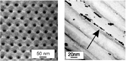
Figure 1: (LEFT) SEM image shows well ordered hexagonal packing of alumina nanopores prepared under similar conditions to samples used for x-ray experiments. (RIGHT) Bright-field TEM image of the nanoparticles (arrow) on the wall (faint diagonal lines) of alumina pores. The nanoparticles are Au-core with octane-thiol coating. Cross-sections were prepared by ultra micro-tome method from the sample used for x-ray experiments.

Nanoporous alumina membranes were further cleaned in solvents to remove organic impurities, with 15 minute ultra-sonic baths in each of the following (in order): HPLC grade chloroform, 99.7% pure acetone, HPLC grade methanol, and HPLC grade toluene. The membrane was then allowed to soak in HPLC grade toluene for 24 hours to remove any further impurities. After soaking, the membrane was transferred without drying to 2 ml of a 2.26 mg/ml solution of octane-thiol (OT) stabilized Au-core nanocrystalsJackson04 ; Terrill95 in HPLC grade toluene for two weeks at 25^∘C. Fits of SAXS data from bulk scattering of a dilute suspension of the same solution of nanoparticles used in doping the nanopores yielded $R_{s}=1.2$ nm and $\Delta_{R}=0.16$ nm giving a polydispersity of $\Delta_{R}/R_{s}=13\%$. Since the electron density of the Au core is much higher than the organic ligands, $R_{s}$ was primarily a measure of the core radius.

The nanoparticle solution was drawn into the alumina pores via capillary forcesBenfield01 ; Sawitowski01 . The initial concentration (and volume) of the nanoparticle solution was chosen such that the total number of particles in the initial solution was about 2-3 times the number of nanoparticles needed to form a complete monolayer of nanoparticles along the walls of the pores (assuming hexagonal close packing), but less than that required for complete volume filling of the pores. In addition to soaking, the solution with the immersed membrane was placed in an ultra-sonic bath for 15 minutes per day to facilitate movement of the particles into the membrane. The long time period and frequent ultra-sonic baths were imposed to ensure maximal integration of nanoparticles into the porous membranes.

After 24 hours in solution the alumina membrane color changed from clear to dark red color, similar to the solution color. This was an indication that nanoparticles had been absorbed into the membrane. The presence of nanoparticles in the pores was confirmed with cross-sectional TEM of the sample (see Fig. 1). No further color changes of the membrane were observed. Additionally, no significant color change of the solution was observed, indicating that some particles were left in the solution. The sample was then removed from the solution and allowed to dry in air for five minutes before being loaded into an environmental chamberTidswell91 ; Heilmann01 (see Fig. 2) for the SAXS experiment.

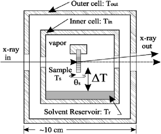
Figure 2: Schematic of the environmental chamber used for in-situ x-ray experiments. The outer (inner) cell was kept at 28^∘C (32^∘C) during the experiment. The sample temperature $T_{s}$ was controlled independently from the inner cell and liquid solvent reservoir temperature, $T_{r}$. The sample was mounted in a transmission geometry where the long axis of the pores can be rotated ($\theta_{s}$) in the horizontal plane. The $\Delta T=T_{s}-T_{r}$ was controlled to vary liquid condensation on the sample via the vapor.

Prior to sample mounting, all components of the inner cell of the environmental chamber were cleaned with solvents: 15 minute ultra-sonic baths of each of HPLC grade chloroform, 99.7% pure acetone, and HPLC grade methanol. During the x-ray experiment the inner cell was hermetically sealed and the temperatures of the inner and outer cells were kept at $T_{in}=32.0\pm 0.5^{\circ}$ C and $T_{out}=28.0\pm 0.5^{\circ}$ C, respectively. The actual temperature stability during each measurement was better than $\pm 50$ mK, though the temperature of the cells did vary $\pm 0.5$ K between different measurements due to the differing heat loads on the sample as described below (see the description of $\Delta T$). The sample mounting block was thermally isolated to a high degree from the walls of the inner cell with independent thermal control via a heater on the mounting block. All temperatures were continuously monitored with YSI #45008 thermistors. A liquid solvent reservoir was created by injecting 10 ml of HPLC grade liquid toluene into the inner cell. Solvent condensation in the sample was precisely controlled via the (positive) offset between the sample temperature, $T_{s}$, and the liquid solvent reservoir temperature, $T_{r}$: $\Delta T=T_{s}-T_{r}$Tidswell91 ; Heilmann01 . The chemical potential offset (from the liquid/vapor coexistence) is given by: $\Delta\mu\approx H_{vap}\Delta T/T_{r}$. Here, $H_{vap}=38.06$ kJ/mol is the heat of vaporization of tolueneMajer85 and $T_{r}$ was kept constant throughout the experiment (as described above) via temperature control of the inner cell. Liquid was injected into the cell at a large $\Delta T\approx 30$ K to avoid rapid condensation in the pores. Since $\Delta T$ could be varied from about 50 mK up to 30 K, the corresponding $\Delta\mu$ could be varied about four orders of magnitude. As $\Delta T$ and thus $\Delta\mu$ decreased the amount of condensed solvent increased. Likewise, solvent was removed by increasing $\Delta T$. In this experiment, the pores became saturated with liquid for all $\Delta T<4$ K, thus the experimental range of $\Delta T$ probed was only 0.5 K$<\Delta T<30$ K. X-rays were allowed to pass through the chamber via 0.02 mm Kapton© (Dupont) windows on the outer chamber and 0.005 inch thick beryllium windows on the inner chamber.

III SMALL ANGLE X-RAY SCATTERING

In-situ x-ray measurements were carried out at the SAXS facility at ChemMatCARS beamline at the Advanced Photon Source (Argonne National Lab, Argonne, IL). The incident x-ray energy of 11.55 keV was well below the L3 absorption edge of Au (11.92 keV) to avoid fluorescence. The sample chamber was mounted on a goniometer in a transmission geometry with two degrees of rotational freedom – sample rotation and tilt – plus the standard three translations. The sample rotation was done internally and allowed rotation angles, $\theta_{s}$, of the sample with respect to the incident beam in excess of $\pm 90^{\circ}$ (see Fig. 2). A fixed position geometry CCD detector measured the SAXS intensity at a camera length, $L$, of 1880 mm down-stream from the sample. Powder diffraction rings were seen at small angles due to the 2D hexagonal packing of the nanopores. Sample alignment was performed with the membrane nearly perpendicular to the incident beam and thus the pores were parallel to the incident beam. The sample rotation and tilt were adjusted to maximize the symmetry of the diffraction rings in both the vertical and horizontal directions. After alignment, the membrane was exactly perpendicular to the incident beam and the long axes of the pores were parallel to the incident beam. This defined $\theta_{s}=90^{\circ}$ between the incident beam and the short axis of the pores. The membrane was then rotated to $\theta_{s}=10\pm 1^{\circ}$ from the incident beam, i.e. the pore long axis was then at 80^∘ to the incident x-rays (see Fig. 3). This geometry allowed a bulk measurement of the nanoparticle/nanopore system while maximizing the wavevector transfer along the nanopore long axis, $q_{z}$, that was probed.

It is important to note that the geometry shown in Fig. 3 is rotated by $90^{\circ}$ about the incident beam for ease of viewing. In the figure, the long axis of the pores is depicted as approximately perpendicular to the incident beam and vertical with rotations $\theta_{s}$ in the vertical plane. In the actual experiment, the only difference was that the long axis of the pore was horizontal (though still perpendicular to the incident beam) and rotations $\theta_{s}$ were done in the horizontal plane.

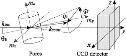
Figure 3: Geometry for SAXS measurements: X-rays were incident at $\theta_{s}=10^{\circ}$ from normal to the nanopore long axis. Scattered intensity was measured with a fixed position CCD detector down-stream. The $\vec{m}$ and $\vec{q}$ describe the coordinate space and wavevector transfer of the nanopore, respectively. Note that the geometry shown here has been rotated about the incident beam by $90^{\circ}$ for clarity.

IV Volume of adsorbed solvent

A measure of absorbed volume of solvent in the pores was calculated from the small angle powder diffraction peaks mentioned above. As liquid was condensed into the pores, the electron density contrast in the pores decreased relative to that of the dry pores, thus reducing the scattering intensity of the diffraction peaks, $I_{peak}(\Delta T)$, relative to the dry peaks, $I_{peak}(dry)$. Neglecting absorption corrections, the added solvent volume, $V_{liq}$, was then approximately determined from the lowest order peak (small angle approximation) viavolume :

$$V_{liq}(\Delta T) \propto \sqrt{I_{peak}(dry)}-\sqrt{I_{peak}(\Delta T)}$$ (1)

Plots of the added volume derived from the $\langle 10\rangle$ diffraction peak are shown in Fig. 4.

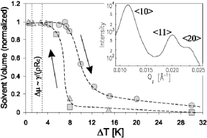
Figure 4: (Main) Volume adsorption($\bigtriangleup,\Box$) / desorption($\bigcirc$) curves as a function of $\Delta T$. Dashed lines are added as a guide for the eye. Note the strong hysteresis upon cycling. Vertical dotted lines indicate location of capillary transition for empty (no nanoparticles) pores predicted by the Kelvin equation, $\Delta\mu\sim\gamma/\rho R_{c}$. Data is normalized to the liquid saturation volume of the pores. (Inset) Plot showing the powder diffraction peaks from the 2D nanopore packing. Volume information was extracted from the first peak (the $\langle 10\rangle$).

The data represent three different thermal cycles: two cooling cycles (large $\Delta T$ to small $\Delta T$) and one heating cycle. The data have been normalized to the saturated (pores completely filled with liquid) volume for each curve. There are two main features in this figure: the first is the presence of a sharp transition (from low relative volume to saturation and reverse) for both adsorption and desorption curves and second, there is a marked hysteresis which is reproducible (at least for the cooling cycle). For both sets of curves, the nanopore/nanoparticle system is saturated with toluene for $\Delta T\leq 4$ K and has negligible amounts of toluene for $\Delta T\geq 30$ K. These two regions will be referred to throughout the rest of the paper as the “saturated” and “dry” regions, respectively.

The simplest theory to describe the observed capillary transition is the Kelvin equation:

$$\Delta\mu_{adsorption} \approx \frac{\gamma}{n_{l}R_{c}}$$ (2)

$$\Delta\mu_{desorption} \approx \frac{2\gamma}{n_{l}R_{c}}$$ (3)

where $R_{c}$ is the cylindrical nanopore radius, $\gamma=28.4$ mN/m is the surface tension of bulk toluene, and $n_{l}=\rho/m_{wt}=9\times 10^{-3}$ moles/cm³ (mass density divided by molecular weight) is the molar density of the toluene. The chemical potential at the capillary transition for the adsorption and desorption differ by a factor of two due to different physical mechanisms for adsorption and desorption. Pores are expected to fill by coaxial film growth (curvature of $1/R_{c}$) and empty from the ends of the pores via a spherical meniscus (curvature of $2/R_{c}$) that travels the length of the pore.Cohan38 This argument provides a motivation for the presence of the hysteresis, even though the system studied is clearly more complicated due to the presence of the nanoparticles. According to the Kelvin equation, the observed capillary filling transition in Fig. 4 would indicate an effective radius for the pores of about 4 nm, almost a factor of four smaller than the actual pore radius of 15 nm. For similar nanoporous alumina samples with no nanoparticles, it was found that the Kelvin equation provides a good prediction of the capillary transitionAlvineUP . Significantly higher values of $\Delta T$ for the capillary transition indicated that there was a real reduction in the effective radius of the pores due to the presence of the nanoparticles. Assuming a monolayer thickness due to the nanoparticles of 2.4 nm for the Au core plus 1.2 nm$\times$2 for the organic OT shellBain89 $\approx 5$ nm, this would bring the effective radius down to about 10 nm. Additionally, roughness from the nanoparticle monolayer surface contributes to the transition shift by increasing the amount of adsorbed liquid at large $\Delta T$Robbins91 .

V Nanoparticle-nanoparticle Scattering

V.1 Elliptical Transforms

In addition to the low angle powder diffraction from the 2D hexagonal pore packing, a ring-like structure was observed at larger angles ($q\approx 0.18$ $\dot{A}^{-1}$, see Fig. 5), which corresponds to nanoparticle interference scattering and contains information about the local packing structure. This scattering ring underwent dramatic changes with the gradual addition, and subsequent removal, of liquid solvent in the pores (see Fig. 6). No sharp diffraction spots were observed upon rotation of the sample through $90^{\circ}$ about the short axis of the pore, indicating that the nanoparticle packing must be powder-like with only short-range order.

To interpret these particle-particle scattering results, it was necessary to transform the scattering intensity from lab (CCD detector) coordinates into the coordinates relative to the nanopore axis as shown in Fig. 5. The transform is given by the constraints of the scattering geometry (see Fig. 3). The wavevector transfer, $\vec{Q}=[Q_{x},Q_{y},Q_{z}]$ is:

$$\vec{Q} = \vec{k}_{inc}-\vec{k}_{scatt}$$ (4)

$$= \frac{k}{\sqrt{x^{2}+z^{2}+L^{2}}}\left[x,L-\sqrt{x^{2}+z^{2}+L^{2}},z\right]$$ (5)

$$\approx \frac{k}{L}\left[x,0,z\right];\ \ L\gg r$$ (6)

Transforming to coordinates of the nanopore (here we use $\vec{q}$, lowercase for clarity), for $\theta_{s}\ll\pi/2$:

$$q_{z} = \frac{\vec{q}\cdot\vec{m_{z}}}{{|m_{z}|}^{2}}\approx\frac{kz\cos{\theta_{s}}}{L}$$ (7)

$$q_{y} = \frac{\vec{q}\cdot\vec{m_{y}}}{{|m_{y}|}^{2}}\approx\frac{kz\sin{\theta_{s}}}{L}$$ (8)

$$q_{x} = \frac{\vec{q}\cdot\vec{m_{x}}}{{|m_{x}|}^{2}}\approx\frac{kx}{L}$$ (9)

$$q_{r} \approx \frac{k\sqrt{x^{2}+z^{2}{\sin}^{2}{\theta_{s}}}}{L};\ L\gg r;\ z\gg\Delta\cot{\theta_{s}}$$ (10)

Here, $\vec{x}=[x,y,z]$ ($\|\vec{x}\>\|=r$) and $\vec{m}=[m_{x},m_{y},m_{z}]$ are the cartesian coordinates of the CCD detector (lab) and nanopore, respectively, and $\Delta=\sqrt{x^{2}+z^{2}+L^{2}}$. The wavevector transfer in the pore coordinates is denoted $\vec{q}$, with magnitude $k=2\pi/\lambda$. In the above approximation, the intersection of the cylindrical surfaces of constant $q_{r}$, and the CCD plane, are ellipses. Fig. 5 shows typical scattering intensity data (upper right) from $\Delta T=30$ K (dry pores). The scattering intensity is transformed into the $q_{z},q_{r}$ coordinates of the nanopore (lower right). The transform excludes data up to $\theta_{s}=10^{\circ}$ from the $q_{z}$ axis (aligned along the nanopore long axis) as a result of the incident angle of the x-rays to the pore axis. Images were taken with the detector off-center to maximize the recorded $q$–range. The triangular region at low q is a result of an attenuator necessary to reduce the intense scattering of the powder diffraction peaks associated with the hexagonal pore-pore packing. The intense scattering concentrated along the $q_{r}$ axis was mainly a result of scattering described by the pore form factor which is narrow in $q_{z}$ due to the length of the pores.

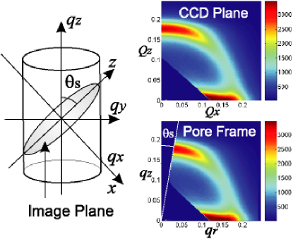
Figure 5: (Color)(Left) Schematic of elliptical transforms of scattering intensity data. Lines of constant $q_{r}$ are ellipses in CCD coordinates where the scattering (CCD) plane intersects the cylindrical surfaces of constant $q_{r}$. (Right Top) CCD image of scattering intensity at $\Delta T=30$ K. The direct beam is in the lower left corner. The triangular region here is due to an attenuator used to block the intense pore-pore scattering at low $q$. (Right Bottom) The same data set transformed to the $\vec{q}$ coordinates relative to the nanopore axis.

The intensity distribution along the nanoparticle scattering ring changed significantly with $\Delta T$. For the dry pores, $\Delta T=30$ K (Fig. 6, upper left) a sharp, strongly asymmetric ring was present, brighter near the $q_{z}$ axis than the $q_{r}$ axis. Here the data have been tiled to all four quadrants to simulate the full ring for ease of viewing. The strong feature along the $q_{r}$ axis was due to the sum of the scattering of the individual pores. The ring asymmetry indicates a structure that is preferentially aligned along the nanopore axis. A model to explain this scattering will be presented in the next section. As liquid was added to the pores (adsorption curve) there was a general trend that the ring became broader and its radius decreased (see Fig. 6, $\Delta T=30~{}\mathrm{K}\rightarrow 8~{}\mathrm{K}\rightarrow 6~{}\mathrm{K}$). This was an indication that the nanoparticle nearest neighbor spacing had increased and the ordering was reduced in comparison with that of the dry case. Upon gradual removal of the liquid (desorption curve) there was a qualitatively different feature that appeared (see Fig. 6, lower left, $\Delta T=12.4$ K).

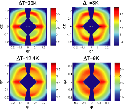
Figure 6: (Color)Scattering intensity distributions at four representative $\Delta T$. Data (intensity log scale) were background subtracted, then tiled into all quadrants to simulate a full ring. (Top Left) Data from $\Delta T=30$ K (dry): the scattering intensity is an asymmetric ring structure from particle-particle scattering. (Top Right) Data from $\Delta T=8$ K (adsorption curve): note the ring is broader with a smaller radius. (Bottom Right) Data from $\Delta T=6$ K (saturated with liquid): here the ring is even broader with an even smaller radius. (Bottom Left) Data from $\Delta T=12.4$ K (desorption curve): note the presence of an isotropic scattering ring just inside the asymmetric ring.

For this value of $\Delta T$, the inner portion of the asymmetric ring was nearly isotropic. This isotropic scattering was an indication of an additional structure of nanoparticle aggregates or clusters. With removal of nearly all of the liquid achieved at the highest $\Delta T$, the scattering again showed a sharp, well defined, asymmetric ring (almost identical to Fig. 6, upper left, $\Delta T=30$ K), indicating that the self-assembly was reversible. The formation of the clusters indicated that there was a form of hysteresis in the self assembly process as well as in liquid adsorption and desorption.

V.2 Nanoparticle Tiling Model

We propose in this section a simple model to describe the scattering from monolayers of Au nanoparticles along the walls of the cylindrical nanopores. Motivation for a self-assembled cylindrical monolayer comes from analogy with self-assembled nanoparticle monolayers on flat substratesNarayanan04 and the attractive van der Waals (vdW) forces between the particles and between the particles and the walls of the nanopore. In the Derjaguin approximation, where the separation, $D$, is much less than the nanoparticle Au-core radius, $R_{s}$, the vdW forces between neighboring nanoparticles, $F_{np-np}$, and between a nanoparticle and the alumina pore wall, $F_{np-wall}$, are:Israel92 ; Ohara95 .

$$F_{np-np} = \frac{A_{nn}R_{s}}{12D^{2}}$$ (11)

$$F_{np-wall} = \frac{A_{nw}R_{s}}{6D^{2}}.$$ (12)

Here, $A_{nn}$ and $A_{nw}$ are the Hamaker constants for the nanoparticle-nanoparticle interaction and nanoparticle-nanopore wall respectively. The Hamaker constants are reduced in the presence of a mediating solvent, but the forces remain attractive. Steric repulsions, due to the OT coating, prevent irreversible nanoparticle aggregation. The attractive vdW forces should partially confine the particles to remain in a monolayer near the walls of the pores. Additionally, inter-particle ordering should be reduced by pore wall roughness and nanoparticle polydispersity. Henderson96 The lack of strong diffraction peaks confirmed that the nanoparticle order was short-range only. There were two distinct length scales involved, the nanoparticle diameter and the nanopore diameter, that differ by an order of magnitude ($\sim 3$ nm to $\sim 30$ nm). Thus, there were two independent scattering regimes: one for low angles, $qR_{c}\stackrel{{\scriptstyle<}}{{\sim}}1$, and another for higher angles, $qR_{s}\stackrel{{\scriptstyle>}}{{\sim}}1$, where $R_{s}$ is the average nanoparticle core radius and $R_{c}$ is the average nanopore radius. For the low angle scattering, which has already been discussed above in the context of added liquid volume, the scattering due to interference from neighboring nanoparticles was ignored for this reason. For the scattering at higher angles, the structure factor associated with the nanopore packing should have decayed to approximately unity (since any pore-pore ordering must be short range in 2D). This high $q$ regime may then be written as the sum of scattering from the pores (as in the low $q$ region, but where now the structure factor is unity) plus a term that describes the local particle-particle scattering. The scattered intensity in the two regimes is given by:

$$I(q) \approx {|S_{p}(q)(F_{s}(q)+F_{p}(q))|}^{2};\quad qR_{c}\stackrel{{\scriptstyle<}}{{\sim}}1$$ (13)

$$I(q) \approx {|F_{p}(q)+S_{np}(q)F_{np}(q)|}^{2};\quad qR_{s}\stackrel{{\scriptstyle>}}{{\sim}}1$$ (14)

Here, $S_{p}$ and $S_{np}$ are the structure factors associated with the local packing of the nanopores and the nanoparticles respectively. $F_{p}$, $F_{s}$, and $F_{np}$ are the form factors associated with the scattering from the nanopores, an average nanoparticle monolayer, and individual nanoparticles respectively. Since the nanopores are about four orders of magnitude longer than their diameter, the scattering associated with them will occur at small $q_{z}$. With the pores almost perpendicular to the direct beam, the intersection of this scattering with the image plane will be such that scattering associated with the pores will be only along the $q_{r}$ axis. The scattering associated with the form factor of the pores is complicated by polydispersity, roughness and the presence of liquid, thus it is treated only as background scattering for this analysis. Strong scattering away from the $q_{r}$ axis must then be attributed to nanoparticle-nanoparticle scattering. Thus away from the $q_{r}$ axis, we may treat the 2nd term in equation (14) as dominant and the first term (and cross term) as a background.

The nanoparticle form factor is described by:

$${|{F_{np}}|}^{2} \propto G(q,R_{s},\Delta_{R}).$$ (15)

where $G(q,R_{s},\Delta_{R})$ is given by the Shulz distributionAragon76 for polydisperse spheres with radius $R_{s}$ and $\Delta_{R}$ defined as the root mean square deviation. For $qR_{s}\stackrel{{\scriptstyle<}}{{\sim}}1$, the nanoparticle form factor is given by the Guinier Law Glatter82 .

$$G(q)\approx\exp(-q^{2}{R_{s}}^{2}/5)$$ (16)

A “tiling” model for calculating $S_{np}(q)$, valid for $qR_{s}\stackrel{{\scriptstyle>}}{{\sim}}1$ is explored below. To model the nanoparticle structure factor for high $q$ (where nanoparticle-nanoparticle interference scattering dominates), the monolayer of particles was broken up into small regions, or tiles, that were approximately flat, as shown in Fig. 7.

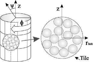
Figure 7: (Left) Schematic of the tiling of the cylindrical nanoparticle monolayer. The monolayer is broken up into small regions, or tiles, which are approximately flat. The scattering is then powder averaged over all tiles at a given orientation $\phi$ from all pores. The total scattering is a sum over all such orientations, $\phi\in[0,2\pi]$. The azimuthal angle is $\psi$ (not to be confused with the sample rotation angle $\theta_{s}$).

The approximation was made that the scattering between individual tiles was independent and that the radius of curvature of the pore is large compared with the inter-particle distance. The first approximation is valid when the dimensions of the tiles are on the order of the average correlation length (order parameter), $\xi$, within the tile or smaller.

The scattering was then powder–averaged over all tiles of a given orientation $\phi$. Thus the scattering intensity from a particular set of tiles at a given $\phi$ was approximately the same as the powder–averaged scattering from a flat monolayer of nanoparticles with an order parameter $\xi$, and nanoparticle nearest neighbor separation $d_{nn}$. A (mathematically) simple Lorentzian model was used to approximate the structure factor, $S^{\phi}$, for each of these orientations:

$${|S^{\phi}_{np}(q,\phi,\psi)|}^{2}\approx$$ (17)

$$\frac{I_{0}\xi}{{1+\xi}^{2}{\left(q\sqrt{(\cos(\psi)-\cos(\phi)\sin(\psi))}-2\pi/d_{nn}\right)}^{2}}.$$

Here $I_{0}$ is an adjustable scale parameter with $I_{0}/d_{nn}$ being proportional to the number of scatters and $\psi$ is the azimuthal angle relative to the long axis of the nanopore (not to be confused with the sample rotation, $\theta_{s}$). Note that if $\xi>d_{nn}$ then $\xi$ may be thought of as the correlation length within the tiles, along the walls of the pore. For $\xi\leq d_{nn}$ then the particles are better described as a 2D dilute, gas-like phase. This analysis only considered the first order peak due to the $q$–range of this experiment, but higher orders would be treated similarly. The total structure factor, $S_{np}$, can be calculated by integrating over all $\phi$.

$${|S_{np}(q,\theta)|}^{2} = \int^{2\pi}_{0}{|S_{np}^{\phi}(q,\phi,\theta)|}^{2}d\phi$$ (18)

The above structure factor, along with the nanoparticle form factor given by the Shulz distribution, was used to fit the high $q$ data of the Au-core nanoparticles in the nanoporous alumina. The CCD data were first flat-field corrected, then background (taken with the sample rotated out of the beam) was subtracted to account for scattering from our environmental chamber windows plus scattering from the toluene vapor. The data were then transformed into the $q_{r},q_{z}$ coordinates of the nanopore as described above. All of the data sets (at different $\Delta T$) fit well with the above described tile model with a monotonic decaying background (which included scattering from both the porous membrane and the liquid) with the exception of the data at $\Delta T=12.4$ K (desorption curve) where an additional isotropic scattering term was necessary for good agreement. This cross-section of the isotropic scattering ring was fit using a Lorentzian with similar parameters as for the monolayer ($\xi,I_{0},$ and $d_{nn}$). For this model, the number of scatters should be proportional to $I_{0}/d_{nn}^{2}$.

For each data set of a given $\Delta T$, a series of representative radial slices was chosen at $\psi_{n}=11\times n^{\circ}$ from the $q_{z}$ axis ($n$ an integer from one to seven), and intensity as a function of $q$ was graphed for each slice (see Fig. 8).

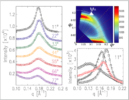
Figure 8: (Color)(Right Top) Schematic of representative radial slices (dashed lines) taken for fitting with the tile model with $\psi_{n}=11\times n^{\circ}$, $n$ an integer from 1 to 7. (Left) Data ($\Box$) at $\Delta T=30$ K from each slice (color coded with dashed lines) along with fits (solid lines) from the tile model plus independent monotonically decaying, positive backgrounds. Error bars are smaller than data symbols. (Bottom Right) Data (all at $\psi_{n}=11^{\circ}$) from four different $\Delta T$: $\Box=30$ K, $\bigtriangleup=8$ K(absorption), $\lozenge=4.4$ K(saturated), and $\bigcirc=12.4$ K(desorption); solid lines are fits. $\Delta T=12.4$ K is qualitatively different and requires an isotropic component in addition to the tile model to fit properly.

Each radial slice was fitted independently with the tiling model plus a monotonically decaying background. As stated above, the main contribution to the background was from the nanopore membrane which increased as $\psi_{n}$ approached 90^∘. This was seen in the fits and thus a slice at 88^∘ was not used due to the fact that the background was greater than the particle-particle scattering. After fitting all of the slices independently, average parameters and uncertainties for each $\Delta T$ were calculated from the mean and standard deviation of each of the three fit parameters: $I_{0}$, $\xi$, and $d_{nn}$. Since the uncertainties were small in comparison to the average value of the parameter, the average parameters were treated as ”best fit” or global parameters for each $\Delta T$.

The three ”best fit” parameters from the tiling model as a function of $\Delta T$ are plotted with uncertainties in Fig. 9. Also plotted in each of the three plots are the parameters from the isotropic component at $\Delta T=12.4$ K ($\blacksquare$). The $\Delta T$ axis is read from left to right; to the left of zero are adsorption (cooling) data, to the right of zero is desorption (heating) data.

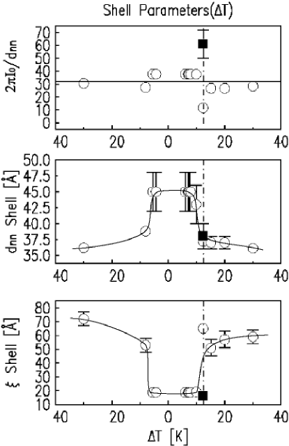
Figure 9: Plots of the ”best fit” tile model ($\bigcirc$) and isotropic ($\blacksquare$) parameters and uncertainties as a function of $\Delta T$ (data to the left of zero are from adsorption curves, to the right are from desorption curves). The physical parameters are (top to bottom): number of scatters $\propto I_{0}/d_{nn}$, nearest neighbor spacing $d_{nn}$, and order parameter $\xi$. Lines are added as a guide to the eye.

The data indicated that the number of nanoparticles in the monolayer, probed by the scattering volume, remained constant as liquid was added and subsequently removed (see Fig. 9, top) with the exception of $\Delta T=12.4$ K where an additional isotropic component was necessary. For this data point, the number of particles in the monolayer decreased. It is likely that some of the missing particles went into the formation of the isotropic clusters. The fact that this data point is higher than the average monolayer number might be indicative that the clusters fill the volume more effectively than the particles in the monolayer.

The formation of these clusters is a surprising phenomenon. Additional isotropic scattering was seen only during desorption and then disappeared upon removal of additional liquid. The formation of clusters, or aggregates may have been linked to the progression of a spherical meniscus through the pores, starting from the ends.Cohan38 As the meniscus travelled through the pore, it would tend to drag particles with it. Another possibility would be the formation of bubbles within the liquid. Upon complete removal of liquid from the system these clusters would dissolve and reassemble into a monolayer structure on the nanopore wall. This is indicated in the data by the disappearance of the isotropic scattering as $\Delta T$ is increased.

The plots in Fig. 9, middle and bottom, demonstrate that with the addition of liquid there was a shift to larger nearest neighbor separation distance with a maximum of 4.5 nm (compared to 3.6 nm for dry), accompanied by a decrease in the order (in the plane of the cylindrical monolayer). Upon removal of the liquid solvent, the particle separation decreased again to the dry value, and the ordering increased back to almost the initial dry value. For relative added liquid solvent volume amounts up to about 0.5 (normalized to saturation; see both Fig. 4 and Fig. 9) the order parameter was about twice that of the nearest neighbor spacing and may be interpreted as an in-plane correlation length. For higher relative amounts of solvent, $V_{liq}>$0.5, the order parameter was less than the nearest neighbor spacing, indicating a 2D dilute gas-like phase.

The value of 3.6 nm for the nearest neighbor spacing for the dry system (large $\Delta T=30$ K) was less than $2(R_{s}+t_{OT})\approx 4.8$ nm, where $t_{OT}\approx 1.2$ nm is the thickness of the OT shell, indicating interdigitation of the shell ligands of neighboring particles. As liquid was absorbed into the organic shells (with decreasing $\Delta T$) the vdW attraction between nanoparticles would decreaseGe00 ; Ohara95 relative to the dry system, while the osmotic pressureSaunders04 between the ligand chains increased, driving the particles apart. This separation increase may have been further facilitated by gaps or voids in monolayer coverage. As liquid filled these gaps, the nanoparticles (undergoing thermal motion) could move into this new volume. Removal of the liquid by increasing $\Delta T$ reduced the repulsive osmotic pressure between the particles and increased the attractive vdW forces, reducing the particle-particle separation.

VI CONCLUSIONS

Low angle measurements established the relative amount of liquid in the nanopores as a function of $\Delta T$. A capillary filling transition occurred between 8 K and 12 K, which was about four times less saturation than what is expected via the Kelvin equation for toluene absorption in pores with no nanoparticles. In addition to the shift, marked hysteresis was also observed.

Fits to the data indicated that the nanoparticles assembled in a cylindrical monolayer aligned along the pore. From the geometry of this structure we conclude that the particles were near the walls, which was physically sensible due to the vdW attraction of the nanoparticles to the nanopore wall. As liquid was added by reducing the relative chemical potential $\Delta\mu$, most of the particles remained in the monolayer structure. Also, the nearest neighbor separation distance increased and the correlation length within the monolayer decreased. The process was reversible: upon removal of the liquid, the nanoparticle nearest neighbor distance decreased to the initial dry value and the ordering increased to almost the dry value.

In addition to the cylindrical monolayer, there was evidence of the formation of isotropic clusters during desorption of the liquid solvent. This phenomenon could have been related to the process by which the liquid emptied from the pore, namely that it was likely to occur from the ends of the pores. This might also explain why this structure was not seen during the adsorption cycle.

We thank Richard Schalek for help with preparing ultra-microtome TEM samples. We also thank Professor Milton Cole for many helpful discussions. This work was supported by the National Science Foundation Grant No. 03-03916. ChemMatCARS Sector 15 is principally supported by the National Science Foundation/Department of Energy under grant number CHE0087817. The Advanced Photon Source is supported by the U.S. Department of Energy, Basic Energy Sciences, Office of Science, under Contract No. W-31-109-Eng-38. Use of the Advanced Photon Source was supported by the U. S. Department of Energy, Office of Science, Office of Basic Energy Sciences, under Contract No. W-31-109-Eng-38.

References

- [1] S. Narayanan, J. Wang, and X. M. Lin. Phys. Rev. Lett. 93, 135503-1 (2004).
- [2] Y. Lu, G. L. Liu, and L. P. Lee. Nano Lett. 5, 5 (2005).
- [3] A. Dokoutchaev, J. T. James, S. C. Koene, S. Pathak, G. K. S. Prakash, and M. E. Thompson. Chem. Mater. 99, 2389 (1999).
- [4] T. Sawitowski, Y. Miquel, A. Heilmann, and G. Schmid. Adv. Funct. Mater. 11, 435 (2001).
- [5] R. E. Benfield, D. Grandjean, M. Kröll, R. Pugin, T. Sawitowski, and G. Schmid. J. Phys. Chem. B 105, 1961 (2001).
- [6] J. Hu, T. W. Odom, and C. M. Lieber. Acc. Chem. Res. 32, 435 (1999).
- [7] R. O. Erickson. Science 181, 705 (1973).
- [8] W. L. Liu, K. Alim, and A. A. Balandin. J. Appl. Phys. Lett. 86, 253108 (2005).
- [9] S. Narayanan, D. R. Lee, R. S. Guico, S. K. Sinha, and J. Wang. Phys. Rev. Lett. 94, 145504-1 (2005).
- [10] E. Rabani, D. R. Relchman, P. L. Geissler, and L. Brus. Nature 426, 271 (2003).
- [11] X. M. Lin, H. M. Jaeger, C. M. Sorensen, and K. J. Klabunde. J. Phys. Chem. B. 105, 3353 (2001).
- [12] P. C. Ohara, D. V. Leff, J. R. Heath, W. M. Gelbart. Phys. Rev. Lett. 75, 3466 (1995).
- [13] G. Ge, and L. Brus. J. Phys. Chem. B. 104, 9573 (2000).
- [14] M. Lahav, T. Sehayek, A. Vaskevich, I. Rubinstein. Angew. Chem. Int. Ed. 42, 5576 (2003).
- [15] W. Mickelson, S. Aloni, W. Q. Han, J. Cumings, and A. Zetti. Science 300, 467 (2003).
- [16] E. A. Kelberg, S. V. Grigoriev, A. I. Okorokov, H. Eckerlebe, N.A. Grigorieva, W. H. Kraan, A. A. Eliseev, A. V. Lukashin, A. A. Vertegel, and K. S. Napolskii. Physica B 335, 123 (2003).
- [17] L. M. Bronstein, D. M. Chernyshov, R. Karlinsey, J. W. Zwanziger, V. G. Matveeva, E. M. Sulman, G. N. Demidenko, H. P. Hentze, and M. Antonietti . Chem. Mater. 15, 2623 (2003).
- [18] Z. Kónya, V. Puntes, I. Kiricsi, J. Zhu, J. W. Ager, III, M. K. Ko, H. Frei, P. Alivisatos, and G. A. Somorjai. Chem. Mater. 15, 1242 (2003).
- [19] H. Masuda and K. Fukuda. Science 268, 1466 (1995).
- [20] H. Xiang, K. Shin, T. Kim, S. I. Moon, T. J. McCarthy, and T. P. Russell. Macromolecules 38, 1055 (2005).
- [21] K. Shin, H. Xiang, S. I. Moon, T. Kim, T. J. McCarthy, and T. P. Russell. Science 306, 76 (2004).
- [22] A. M. Jackson, J. W. Myerson, and F. Stellacci. Nature Mater. 3, 330 (2004).
- [23] R. H. Terrill, T. A. Postlethwaite, C. Chen, C. Poon, A. Terzis, A. Chen, J. E. Hutchison, M. R. Clark, G. Wignall, J. D. Londono, R. Superfine, M. Falvo, C. S. Johnson Jr., E. T. Samulski, and R. W. Murray. J. Am. Chem. Soc. 117, 12537 (1995).
- [24] I. M. Tidswell, T. A. Rabedeau, P. S. Pershan, and S. D. Kosowsky. Phys. Rev. Lett. 66, 2108 (1991).
- [25] R. K. Heilmann, M. Fukuto and P. S. Pershan. Phys. Rev. B 63, 205405 (2001).
- [26] V. Majer and V. Svoboda. Enthalpies of Vaporization of Organic Compounds: A Critical Review and Data Compilation, Blackwell Scientific Publications, Oxford, UK 1985, pp 300.
- [27] This is a result of the approximation of the form factor for small wavevector transfer:
- [28] L. H. Cohan. J. Am. Chem. Soc. 60, 433 (1938).
- [29] K. J. Alvine, O. Shpyrko, P. S. Pershan, K. Shin, and T. P. Russell. ”unpublished work” (2005).
- [30] C. D. Bain, E. B. Troughton, Y. T. Tao, J. Evall, G. M. Whitesides, and R. G. Nuzzo. J. Am. Chem. Soc. 111, 321 (1989).
- [31] M. O. Robbins, D. Andelman, and J. F. Joanny. Phys. Rev. A. 43, 4344 (1991).
- [32] J. M. Israelachvili. Intermolecular & Surface Forces, 2nd ed., (Academic Press, New York, USA, 1992)
- [33] S. I. Henderson, T. C. Mortensen, S. M. Underwood, and W. van Megen. Physica A 233, 102 (1996).
- [34] S.R. Aragón and R. Pecora. J. Chem. Phys. 64, 2395 (1976).
- [35] O. Glatter and O. Kratky. Small angle x-ray scattering, (Academic Press, New York, USA, 1982)
- [36] A. E. Saunders, B. A. Korgel. J. Phys. Chem. B. 108, 16732 (2004).