Kinetics of the superconducting charge qubit in the presence of a quasiparticle

Abstract

We investigate the energy and phase relaxation of a superconducting qubit caused by a single quasiparticle. In our model, the qubit is an isolated system consisting of a small island (Cooper-pair box) and a larger superconductor (reservoir) connected with each other by a tunable Josephson junction. If such a system contains an odd number of electrons, then even at lowest temperatures a single quasiparticle is present in the qubit. Tunneling of a quasiparticle between the reservoir and the Cooper-pair box results in the relaxation of the qubit. We derive master equations governing the evolution of the qubit coherences and populations. We find that the kinetics of the qubit can be characterized by two time scales - quasiparticle escape time from the reservoir to the box $\Gamma_{\textrm{in}}^{-1}$ and quasiparticle relaxation time $\tau$. The former is determined by the dimensionless normal-state conductance $g_{{}_{T}}$ of the Josephson junction and one-electron level spacing $\delta_{r}$ in the reservoir ($\Gamma_{\textrm{in}}\!\sim\!g_{{}_{T}}\delta_{r}$), and the latter is due to the electron-phonon interaction. We find that phase coherence is damped on the time scale of $\Gamma_{\textrm{in}}^{-1}$. The qubit energy relaxation depends on the ratio of the two characteristic times $\tau$ and $\Gamma_{\textrm{in}}^{-1}$ and also on the ratio of temperature $T$ to the Josephson energy $E_{{}_{J}}$.

I Introduction

Recent experiments with superconducting charge qubits demonstrated coherent oscillations between two charge states of a superconducting island, a so-called Cooper-pair box (CPB), in a single-electron device Nakamura ; Wallraff ; Vion ; Blais . A device with a large superconducting gap $\Delta>E_{c}>E_{{}_{J}}\gg T$ can be controlled with the gate voltage and magnetic flux, and has only one discrete degree of freedom: the number of Cooper pairs in the box. (Here $E_{c}$ is the charging energy of the island, and $E_{{}_{J}}$ is an effective Josephson energy of its junctions with the reservoir; $E_{{}_{J}}$ can be tuned by the flux.) The practical implementation of superconducting qubits requires long coherence times DiVincenzo . Although the contribution of the quasiparticles to the decoherence of the existing qubits is not the leading one Devoret ; Astafiev , it limits qubit operations on the fundamental level. This motivates us to study the qubit dynamics in the presence of a quasiparticle.

In this paper we consider energy and phase relaxation in a superconducting charge qubit due to the presence of a single quasiparticle. Passing of a quasiparticle through the Josephson junction leads to the escape of the qubit out of a two-level system Hilbert space, and thus determines the decay rate of coherent oscillations. In a previous paper Lutchyn , we evaluated rates of the elementary acts involving quasiparticle tunneling. In particular, we showed that the rate of tunneling into the CPB $\Gamma_{\textrm{in}}$ is determined by the dimensionless (in units of $e^{2}/h$) conductance $g_{{}_{T}}$ of the junction between the CPB and the reservoir, and level spacing in the reservoir $\Gamma_{\textrm{in}}\sim g_{{}_{T}}\delta_{r}/4\pi$. The rate of tunneling out of CPB is $\Gamma_{\textrm{out}}\sim g_{{}_{T}}\delta_{b}/4\pi$ with $\delta_{b}$ being level spacing in the box. Taking into account the difference in the volumes ($V_{r}\gg V_{b}$), one can notice that $\Gamma_{\textrm{out}}\gg\Gamma_{\textrm{in}}$. Therefore, for a sufficiently small box the quasiparticle dwelling time in the CPB is very short, and the qubit spends most of the time in the “good” part of the Hilbert space. Nevertheless, the evolution of the qubit will be affected by quick “detours” the qubit takes outside that part of the Hilbert space. We demonstrate that even a single detour destroys the coherence of the qubit. Combined with the phonon-induced relaxation of the non-equilibrium quasiparticle in the reservoir, the detours also lead to the relaxation of the populations of the qubit states. We derive and solve the master equations for the dynamics of the qubit, which describe its relaxation caused by a quasiparticle.

The paper is organized as follows. We begin in Sec. II with a qualitative discussion and brief overview of the main results. In Sec. III we derive the microscopic master equations for the dynamics of the qubit without quasiparticle relaxation. We solve these equations and discuss the kinetics of the coherences and populations in the Sec. IV and V. In Sec. VI we incorporate mechanisms of quasiparticle relaxation into the master equations and solve them for fast and slow quasiparticle relaxation limits. Finally, in Sec. VII we summarize our main results.

II Qualitative Considerations and Main Results

Dynamics of the superconducting charge qubit is conventionally described by an effective Hamiltonian Shnirman

$$H_{\textrm{qb}}=E_{c}(N-N_{g})^{2}+H_{{}_{J}},$$ (1)

where $E_{c}$ is charging energy of the box, $N$ is the charge of the CPB in units of one-electron charge $e$, and $N_{g}$ is the dimensionless gate voltage. The Hamiltonian of Cooper-pair tunneling $H_{{}_{J}}$ is defined as $H_{{}_{J}}=-\frac{E_{{}_{J}}}{2}\left(\left|N+2\right>\left<N\right|+H.c.\right)$, where $E_{{}_{J}}$ is the Josephson energy. In the case of a large superconducting gap

$$\Delta>E_{c}>E_{{}_{J}}\gg T,$$

the existence of quasiparticles is usually neglected, and the dynamics of the system is described by Hamiltonian (1) with only one discrete degree of freedom, the excess number of Cooper pairs in the box. The qubit can first be prepared in a state with an integer number of pairs in the CPB, e.g., in state $\left|N\right>$ with even $N$, and then tuned to the operating point by adjusting the gate voltage to the value $N_{g}=N+1$. The charge degeneracy between states $\left|N\right>$ and $\left|N+2\right>$ at this point is lifted by the Josephson tunneling, and the states of the qubit are described by the symmetric and antisymmetric superposition of the charge states, $\left|-\right>=\frac{\left|N\right>+\left|N+2\right>}{\sqrt{2}}$ and $\left|+\right>=\frac{\left|N\right>-\left|N+2\right>}{\sqrt{2}}$ with energies

$$\omega_{-}=E_{c}-E_{{}_{J}}/2\mbox{ and }\omega_{+}=E_{c}+E_{{}_{J}}/2,$$ (2)

respectively. Other charge states have much higher energy, and effectively the Cooper-pair box reduces to a two-level system. Being coherently excited by such tuning, the qubit oscillates between the states $\left|+\right>$ and $\left|-\right>$ with the frequency defined by the Josephson energy $E_{{}_{J}}$.

The presence of a quasiparticle with a continuum excitation spectrum provides a channel for relaxation of the qubit. If the state $\left|N\right>$ is prepared in equilibrium conditions, then the quasiparticle resides in the reservoir part Lutchyn of the qubit. Upon tuning of the qubit from state $\left|N\right>$ to the operating point, a charge degeneracy point for the system is passed at $N_{g}=N+1/2$, see Fig. 1. (Hereafter we assume equal superconducting gap energies in the reservoir and Cooper-pair box.) However, if tuning is performed fast enough, the quasiparticle remains in the reservoir Guillaume .

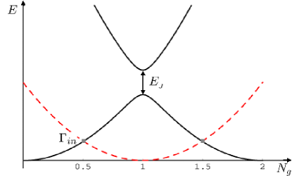
Figure 1: (color online). Energy of the Cooper-pair box as a function of dimensionless gate charge $N_{g}$ in units of $e$ (solid line). Near the degeneracy point ($N_{g}=1$) Josephson coupling mixes charge states and modifies the energy of the CPB. The dashed line corresponds to the charging energy of the CPB with an unpaired electron in the box. At $N_{g}=0.5$, the tunneling rate $\Gamma_{\textrm{in}}$ lifts the degeneracy between the ground state of the CPB (solid line) and a state with a single quasiparticle in CPB (dashed line). We assume equal superconducting gap energies in the reservoir and CPB.

The coherent charge oscillations at the operating point of the qubit continue until the particle finds its way into the CPB. On average, this occurs on a time scale of the order of $(g_{{}_{T}}\delta_{r}/4\pi)^{-1}$. There are several assumptions that allow for this estimate Lutchyn . First, the quasiparticle level spacings $\delta_{b}$ and $\delta_{r}$ in the CPB and reservoir, respectively, must be small compared with the temperature $T$, which defines the initial width of the energy distribution of the quasiparticle. Second, the fluctuations of the potential between the grains must exceed $\delta_{r}$, see, e.g., Ref. [Blanter, ]. Third, we neglected the difference between $\Delta$ and $E_{c}$ when including in the estimate the density of states and tunneling matrix elements of a quasiparticle at energy $\sim E_{c}$ above the gap in the CPB. Under these conditions, the average time it takes the quasiparticle to leave the reservoir and enter the CPB is of the order of the inverse level width of a state in the reservoir with respect to leaving it through the junction of conductance $g_{{}_{T}}$

$$\Gamma_{\textrm{in}}^{-1}\sim\left(\frac{g_{{}_{T}}\delta_{r}}{4\pi}\right)^{-1}.$$ (3)

Once the quasiparticle enters the CPB, the charging energy that the qubit has at operation point is transformed into the kinetic energy of the quasiparticle, see Fig. 1. The quasiparticle may escape the CPB leaving the qubit in the excited or ground state, see Fig. 2. The rates of escape into these states are different due to the difference of the kinetic energies available to the quasiparticle upon the escape and due to the energy dependence of the superconducting density of states $\nu(\varepsilon)$. If the qubit ends up in the excited state upon the escape, then only energy $\varepsilon\sim T$ is available for the quasiparticle, and $\nu(T)\sim\delta_{r}^{-1}(\Delta/T)^{1/2}$ (we used here the condition $\Delta\gg T$). The corresponding escape rate is

$$\Gamma_{\textrm{out}}^{{}_{\left|+\right>}}\sim\frac{g_{{}_{T}}\delta_{b}}{4\pi}\sqrt{\frac{\Delta}{T}}.$$ (4)

If the qubit arrives in the ground state, then energy $\sim E_{{}_{J}}$ is available to the quasiparticle, and its density of states in the final state is $\nu(E_{{}_{J}})\sim\delta_{r}^{-1}(\Delta/E_{{}_{J}})^{1/2}$; the rate of escape to this state is

$$\Gamma_{\textrm{out}}^{{}_{\left|-\right>}}\sim\frac{g_{{}_{T}}\delta_{b}}{4\pi}\sqrt{\frac{\Delta}{E_{{}_{J}}}}.$$ (5)

These two rates are much higher than $\Gamma_{\textrm{in}}$ because $\delta_{b}\gg\delta_{r}$, so detours of the quasiparticle to the CPB are short compared to the time quasiparticle spends in the reservoir. Nevertheless, the typical time the quasiparticle spends in the CPB is much greater than the oscillation period of the qubit. Indeed, the ratio

$$\frac{\Gamma_{\textrm{out}}^{{}_{\left|-\right>}}}{E_{{}_{J}}}\sim\frac{\delta_{b}}{\Delta}\sqrt{\frac{\Delta}{E_{{}_{J}}}}$$ (6)

is small: $\delta_{b}/\Delta\sim 10^{-4}-10^{-3}$ for any reasonable size of the CPB (we used here the Ambegaokar-Baratoff relation between $E_{{}_{J}}$, $g_{{}_{T}}$ and $\Delta$). The times of return of the quasiparticle back to the reservoir are randomly distributed. The probability of the quasiparticle returning to the reservoir during times that are short compared to the oscillation period $2\pi/E_{{}_{J}}$ is of the order $\Gamma_{\textrm{out}}/E_{{}_{J}}$ and is small (here we do not distinguish between $\Gamma_{\textrm{out}}^{{}_{\left|-\right>}}$ and $\Gamma_{\textrm{out}}^{{}_{\left|+\right>}}$). Therefore, a single detour of the quasiparticle into the CPB destroys coherent oscillations of the qubit with overwhelming probability. Taking into account the relation $\Gamma_{\textrm{in}}\ll\Gamma_{\textrm{out}}^{\pm}$, we find that the dephasing rate for the qubit, induced by the quasiparticle, is limited by the rate of quasiparticle tunneling into the CPB

$$\frac{1}{T_{2}}\sim\Gamma_{\textrm{in}}$$ (7)

with $\Gamma_{\textrm{in}}$ of Eq. (3).

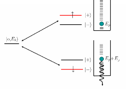
Figure 2: (color online). Schematic picture of the transitions between the qubit states in the presence of a quasiparticle in the reservoir, e.g. $\left|+,E_{p}\right>\leftrightarrow\left|\mbox{\rm{o}},E_{k}\right>.$ Having kinetic energy $\sim E_{{}_{J}}$ the quasiparticle can emit a phonon. The corresponding state of the system is $\left|-,E_{p}\!+\!E_{{}_{J}}\right>$.

Unlike the phase, the energy stored in the degrees of freedom described by the qubit Hamiltonian (1) is not dissipated at the short time scale given by Eq. (7). We start analyzing the time evolution of the qubit energy by considering the limit of infinitely slow quasiparticle relaxation (the latter typically is determined by the electron-phonon interaction Kaplan ; Clarke ). If initially the system was prepared in the $\left|+\right>$ state, then upon a single cycle of quasiparticle tunneling, the qubit ends up in the ground state with a small probability defined by the ratio $\Gamma_{\textrm{out}}^{{}_{\left|-\right>}}/\Gamma_{\textrm{out}}^{{}_{\left|+\right>}}\sim\sqrt{T/E_{{}_{J}}}$. In other words, the qubit energy will randomly change over time between two values $\omega_{+}$ and $\omega_{-}$, see Eq. (2). The portion of the time, the qubit spends in the ground state and the quasiparticle is excited to the energy $E_{{}_{J}}$ above the gap, is small $\sim\sqrt{T/E_{{}_{J}}}$.

The portion of time that the quasiparticle spends in an excited state in the reservoir becomes important when we account for the phonon-induced relaxation of the quasiparticle. Having energy $E_{{}_{J}}$, the quasiparticle may emit a phonon at some rate $1/\tau$ and relax to a low-energy state. The relaxation of the quasiparticle will prevent further reexcitation of the qubit into $\left|+\right>$ state and result in qubit energy relaxation. To find the energy relaxation rate of the qubit, we multiply the portion of time the quasiparticle spends in the excited state by the relaxation rate $1/\tau$:

$$\frac{1}{T_{1}}\sim\sqrt{\frac{T}{E_{{}_{J}}}}\frac{1}{\tau}.$$ (8)

This estimate is applicable if $\tau\gg 1/\Gamma_{\textrm{in}}$, and many cycles occur before the energy is dissipated into the phonon bath.

In the opposite case of fast relaxation $\tau\ll 1/\Gamma_{\textrm{in}}$, the quasiparticle loses its energy the first time it gets it from the degrees of freedom of the Hamiltonian (1). Therefore, in this case the qubit energy relaxation on average occurs on the time scale

$$\frac{1}{\widetilde{T}_{1}}\sim\sqrt{\frac{T}{E_{{}_{J}}}}\Gamma_{\textrm{in}}.$$ (9)

For aluminum, a typical superconductor used for charge qubits, the quasiparticle relaxation time $\tau$ is indeed determined by the inelastic electron-phonon scattering Kaplan ; Clarke , and at low energies ($\varepsilon\leq E_{{}_{J}}$) it can be estimated as $\tau\!\gtrsim 10\,\mu s$. For a small mesoscopic superconductor this time is longer than the typical values of $1/\Gamma_{\textrm{in}}$, and Eq. (8) gives an adequate estimate for the qubit energy relaxation rate.

A comparison of the phase relaxation time (7) with even the shortest of the two energy relaxation times (9), indicates that the coherence is destroyed much earlier than the populations of the qubit states approach equilibrium. Therefore one may consider the decay of qubit coherence separately from the process of equilibration, which involves the electron-phonon interaction in addition to the quasiparticle tunneling. In the rest of the paper, we derive and solve the master equations, which yield results discussed qualitatively in this section.

III Derivation of the Master Equations without quasiparticle relaxation.

The Hamiltonian of the entire system consists of the qubit Hamiltonian $H_{\textrm{qb}}$, BCS Hamiltonians for the superconducting box and reservoir $H_{{}_{\textrm{BCS}}}^{b}$ and $H_{{}_{\textrm{BCS}}}^{r}$, respectively, and quasiparticle tunneling Hamiltonian $V$:

$$H=H_{0}+V,$$ (10)

where $H_{0}=H_{{}_{\textrm{BCS}}}^{b}+H_{{}_{\textrm{BCS}}}^{r}+H_{\textrm{qb}}$ and perturbation Hamiltonian $V$ takes into account only tunneling of quasiparticles $V=H_{{}_{T}}\!-\!H_{{}_{{}_{J}}}$. The tunneling Hamiltonian $H_{{}_{T}}$ is defined as

$$H_{{}_{T}}=\sum_{kp\sigma}(t_{kp}c_{k,\sigma}^{{\dagger}}c_{p,\sigma}+\emph{h.c.}),$$ (11)

where $t_{kp}$ is the tunneling matrix element, $c_{k,\sigma}$, $c_{p,\sigma}$ are the annihilation operators for an electron in the state $k,\sigma$ in the CPB and state $p,\sigma$ in the superconducting reservoir, respectively; $H_{{}_{J}}$ is of the second order in tunneling amplitude footnote

$$H_{{}_{J}}=\left|N\right>\left<N\right|H_{{}_{T}}\frac{1}{E-H_{0}}H_{{}_{T}}\left|N\!+2\right>\left<N\!+2\right|+H.c.$$ (12)

The matrix element $\left<N\right|H_{{}_{T}}\frac{1}{E-H_{0}}H_{{}_{T}}\left|N+2\right>$ is proportional to effective Josephson energy $E_{{}_{J}}$, and $H_{{}_{T}}$ is defined in Eq. (11). Without quasiparticles Hamiltonian $H_{0}$ reduces to Eq. (1), and qubit dynamics can be described using the states $\left|+\right>$ and $\left|-\right>$. In the presence of a quasiparticle, qubit phase space should be extended. Relevant states now are $\left|+,E_{p}\right>$, $\left|-,E_{p}\right>$, and $\left|\mbox{\rm{o}},E_{k}\right>$. The first two states $\left|\pm,E_{p}\right>$ correspond to qubit being in the excited (ground) state $\left|\pm\right>$ and a quasiparticle residing in the reservoir with energy $E_{p}=\sqrt{\xi_{p}^{2}+\Delta^{2}}$:

$$\left|\pm,E_{p}\right>\equiv\left|\pm\right>\otimes\left|E_{p}\right>.$$

The third state $\left|\mbox{\rm{o}},E_{k}\right>$ describes the qubit in the “odd” state with $N\!+1$ electrons in the box, i.e., the qubit escapes outside of its two-level Hilbert space. Here $E_{k}=\sqrt{\xi_{k}^{2}+\Delta^{2}}$ is the energy of the quasiparticle in the box. Perturbation Hamiltonian $V$ causes transitions between the states $\left|\pm,E_{p}\right>$ and $\left|\mbox{\rm{o}},E_{k}\right>$, see Fig. 2. Note that $V$ does not induce the transitions between $\left|+,E_{p}\right>$ and $\left|-,E_{p}\right>$.

The evolution of the full density matrix of the system is described by Heisenberg equation of motion ($\hbar=1$):

$$\dot{\rho_{I}}(t)=-i[V_{{}_{I}}(t),\rho_{{}_{I}}(t)],$$ (13)

where subscript $I$ stands for the interaction representation, i.e., $V_{{}_{I}}(t)=e^{iH_{0}t}Ve^{-iH_{0}t}$. The iterative solution of Eq. (13) yields for the matrix elements of the density matrix

$$\!\left<s\right|\dot{\rho}_{{}_{I}}(t)\!\left|s^{\prime}\right>\! \!=\! \!-i\left<s\right|[V_{{}_{I}},\rho(0)]\left|s^{\prime}\right>$$

$$\!-\! \!\int_{0}^{t}\!{d\tau}\!\left<s\right|\!\left[V_{{}_{I}}(t),[V_{{}_{I}}(t\!-\!\tau),\rho_{{}_{I}}(t\!-\!\tau)]\right]\!\left|s^{\prime}\right>\!,$$

where $\left|s\right>$ can be $\left|+,E_{p}\right>$, $\left|-,E_{p}\right>$, or $\left|\mbox{\rm{o}},E_{k}\right>$. The interaction Hamiltonian $V$ has no diagonal elements in the representation for which $H_{0}$ and $\rho(0)$ are diagonal. Therefore, the first term in right-hand side of Eq. (III) is equal to zero,

$$\!\left<s\right|\dot{\rho}_{{}_{I}}(t)\!\left|s^{\prime}\right>\!\!=\!-\!\!\int_{0}^{t}\!{d\tau}\!\left<s\right|\!\left[V_{{}_{I}}(t),[V_{{}_{I}}(t\!-\!\tau),\rho_{{}_{I}}(t\!-\!\tau)]\right]\!\left|s^{\prime}\right>\!.$$

Equation (III) implies that evolution of the projected density matrix is proportional to $V^{2}$. Since interaction is assumed to be weak, the rate of change of $\rho_{{}_{I}}(t\!-\!\tau)$ is slow compared to that of $V_{{}_{I}}(t)$. Therefore, one can approximate $\rho_{{}_{I}}(t\!-\!\tau)$ by $\rho_{{}_{I}}(t)$ in the right-hand side of Eq. (III) (see, for example, Refs. [Zubarev, ; Esposito, ] for more details on the derivation). Finally, going back to the original representation, we arrive at the following system of master equations

$$\!\left<s\right|\! \!\dot{\rho}(t)\left|s^{\prime}\right>=-\!i\left<s\right|(E_{s}\!-\!E_{s^{\prime}})\rho(t)\left|s^{\prime}\right>$$

$$\!-\! \!\pi\sum_{m,n}\left<s\right|V\left|m\right>\left<m\right|V\left|n\right>\left<n\right|\rho(t)\left|s^{\prime}\right>\delta(E_{n}\!-\!E_{m})$$

$$\!-\! \!\pi\sum_{m,n}\left<s\right|\rho(t)\left|m\right>\left<m\right|V\left|n\right>\left<n\right|V\left|s^{\prime}\right>\delta(E_{m}\!-\!E_{n})$$

$$\!+\! \!\pi\sum_{m,n}\left<s\right|V\left|m\right>\left<m\right|\rho(t)\left|n\right>\left<n\right|V\left|s^{\prime}\right>\delta(E_{n}\!-\!E_{s^{\prime}})$$

$$\!+\! \!\pi\sum_{m,n}\left<s\right|V\left|m\right>\left<m\right|\rho(t)\left|n\right>\left<n\right|V\left|s^{\prime}\right>\delta(E_{m}\!-\!E_{s}),$$

where states $\left|m\right>$, $\left|n\right>$, $\left|s\right>$, and $\left|s^{\prime}\right>$ denote $\left|+,E_{p}\right>$, $\left|-,E_{p}\right>$, or $\left|\mbox{\rm{o}},E_{k}\right>$, and the sum runs over all possible configurations. The system of equations (III) describes the kinetics of the qubit in the presence of a quasiparticle in the Markovian approximation. We are interested in elements of the density matrix that are diagonal in quasiparticle subspace, e.g., $P_{{}_{\!+-\!}}(E_{p},t)=\left<\!+,E_{p}\right|\rho(t)\left|E_{p},-\right>$, since at the end one should take the trace over quasiparticle degrees of freedom to obtain observable quantities. Note that Eq. (III) which describes evolution of a closed system (the qubit and the quasiparticle) does conserve its total energy. We will include the mechanisms of energy loss to the phonon bath and discuss the proper modifications of the master equation later in Sec. VI.

We now apply secular approximation to Eq. (III). This is justified due to the separation of the characteristic time scales $E_{{}_{J}}^{-1}\ll\Gamma_{\textrm{out}}^{-1}\ll\Gamma_{\textrm{in}}^{-1}$ established in the previous section. When considering the evolution of the off-diagonal elements of the density matrix $P_{{}_{\!+-\!}}(E_{p},t)$, we need to keep only terms $\propto P_{{}_{\!+-\!}}(E_{p},t)$ in the right-hand-side of the corresponding master equation. The contribution of other elements of the density matrix to the evolution of the coherences $P_{{}_{\!+-\!}}(E_{p},t)$ is small as $\Gamma_{\textrm{out}}/E_{{}_{J}}$ and $\Gamma_{\textrm{in}}/E_{{}_{J}}$. Thus, we arrive at the equation governing the evolution of the coherences

$$\dot{P}_{{}_{{\!+-\!}}}(E_{p},t)\! \!=\! \!-iE_{{}_{J}}P_{{}_{\!+-\!}}(E_{p},t)$$

$$\!-\! \!\frac{1}{2}\sum_{k}\left[W_{\textrm{+}}(E_{p},E_{k})+W_{\textrm{-}}(E_{p},E_{k})\right]P_{{}_{\!+-\!}}(E_{p},t).$$

The transition rates $W_{\textrm{+}}(E_{p},E_{k})$ and $W_{\textrm{-}}(E_{p},E_{k})$ are given by the Fermi golden rule

$$W_{\textrm{+}}(E_{p},\!E_{k})\!=\!2\pi|\left<E_{p},\!+\right|H_{{}_{T}}\left|\mbox{\rm{o}},E_{k}\right>|^{2}\delta(E_{p}\!+\!\omega_{+}\!-\!E_{k})$$

$$W_{\textrm{-}}(E_{p},\!E_{k})\!=\!2\pi|\left<E_{p},\!-\right|H_{{}_{T}}\left|\mbox{\rm{o}},E_{k}\right>|^{2}\delta(E_{p}\!+\!\omega_{-}\!-\!E_{k})$$

with $\omega_{\pm}$ of Eq. (2). The matrix elements $\left<E_{p},\pm\right|H_{T}\left|\mbox{\rm{o}},E_{k}\right>$ can be calculated using the particle conserving version of the Bogoliubov transformation Schrieffer and are $\left<E_{p},\pm\right|H_{T}\left|\mbox{\rm{o}},E_{k}\right>=\sqrt{2}(t_{pk}u_{p}u_{k}-t_{kp}v_{p}v_{k})$, where $u_{p}$, $v_{p}$ are Bogoliubov coherence factors:

$$u_{p}^{2}=\frac{1}{2}\left(1+\frac{\xi_{p}}{E_{p}}\right),\mbox{ and }v_{p}^{2}=\frac{1}{2}\left(1-\frac{\xi_{p}}{E_{p}}\right),$$ (19)

leading to Tinkham

$$W_{\textrm{+}}(E_{p},\!E_{k})\!=\!2\pi|t_{pk}|^{2}\!\left(\!1\!+\!\frac{\xi_{p}\xi_{k}\!-\!\Delta^{2}}{E_{p}E_{k}}\!\right)\!\delta(E_{p}\!+\!\omega_{+}\!-\!E_{k}),$$

$$W_{\textrm{-}}(E_{p},\!E_{k})\!=\!2\pi|t_{pk}|^{2}\!\left(\!1\!+\!\frac{\xi_{p}\xi_{k}\!-\!\Delta^{2}}{E_{p}E_{k}}\!\right)\!\delta(E_{p}\!+\!\omega_{-}\!-\!E_{k}).$$

Now we may relate the tunneling matrix elements to the normal-state junction conductance

$$g_{{}_{T}}=8\pi^{2}\sum_{p,k}|t_{pk}|^{2}\delta(\xi_{p})\delta(\xi_{k}).$$

Assuming that tunnel matrix elements $t_{pk}$ are weakly dependent on the energies $\xi_{k}$, $\xi_{p}$, we can rewrite Eq. (III) in terms of the dimensionless conductance:

$$W_{\textrm{+}}(E_{p},\!E_{k})\!=\!\frac{g_{{}_{T}}\delta_{r}\delta_{b}}{4\pi}\!\left(\!1\!+\!\frac{\xi_{p}\xi_{k}\!-\!\Delta^{2}}{E_{p}E_{k}}\!\right)\!\delta(E_{p}\!+\!\omega_{+}\!-\!E_{k}),$$

$$W_{\textrm{-}}(E_{p},\!E_{k})\!=\!\frac{g_{{}_{T}}\delta_{r}\delta_{b}}{4\pi}\left(\!1\!+\!\frac{\xi_{p}\xi_{k}\!-\!\Delta^{2}}{E_{p}E_{k}}\!\right)\!\delta(E_{p}\!+\!\omega_{-}\!-\!E_{k}),$$

where $\delta_{r(b)}$ is mean level spacing in the reservoir(box) $\delta_{r(b)}=(\nu_{r(b)}V_{r(b)})^{-1}$ with $\nu_{r(b)}$ being single-spin electron density of states at the Fermi level in the reservoir (box).

The system of equations for the diagonal part of the density matrix describes the evolution of the populations and follows from Eq. (III). From now on we adopt the short-hand notation for the diagonal elements of the density matrix $\left<s\right|\rho(t)\left|s\right>=P_{ss}(E_{s},t)$. In particular, we denote the probability of the qubit to be in the state $\left|+\right>$ or in the state $\left|-\right>$ and a quasiparticle to have energy $E_{p}$ as $P_{++}(E_{p},t)$ or $P_{--}(E_{p},t)$, respectively; the probability $P_{\textrm{o}}(E_{k},t)$ corresponds to the state with a quasiparticle residing in the CPB and having energy $E_{k}$. In these notations the system of equations describing the dynamics of the populations for the states $\left|+,E_{p}\right>$, $\left|-,E_{p}\right>$ or $\left|\mbox{\rm{o}},E_{k}\right>$ can be written as

$$\!\dot{P}_{{}_{\textrm{++}}}\!(\!E_{p},\!t)\!\!+\!\sum_{k}W_{\textrm{+}}(E_{p},E_{k})\left[P_{{}_{\textrm{++}}}(E_{p},t)\!-\!P_{\textrm{o}}(E_{k},t)\right]\!=\!0,\!\\$$ (22a)

$$\!\dot{P}_{\textrm{-\,-}}(E_{p},\!t)\!+\!\sum_{k}W_{\textrm{-}}(E_{p},E_{k})\left[P_{\textrm{-\,-}}(E_{p},t)\!-\!P_{\textrm{o}}(E_{k},t)\right]\!=0,\!\\$$ (22b)

$$\!\dot{P}_{\textrm{o}}(E_{k},\!t)\!\!+\!\!\sum_{p}\left[W_{\textrm{\!+\!}}(E_{p},E_{k})\!+\!W_{\textrm{-}}(E_{p},E_{k})\right]P_{\textrm{o}}(E_{k},t)\!-\!$$

$$\!-\!\sum_{p}\!\left[W_{\textrm{+}}\!(\!E_{p},\!E_{k})P_{{}_{\textrm{\!++\!}}}\!(\!E_{p},\!t)\!+\!W_{\textrm{-}}\!(\!E_{p},\!E_{k})P_{\textrm{-\,-}}\!(\!E_{p},\!t)\right]\!=\!0,\!$$

where we neglected the contribution of the coherences. This is justified as long as $P_{{}_{\!+-\!}}(E_{p},0)=0$ in the initial moment of time, and the two parameters $\Gamma_{\textrm{out}}/E_{{}_{J}}$ and $\Gamma_{\textrm{in}}/E_{{}_{J}}$, are small. The transition rates in Eqs. (22) are given by the Fermi golden rule, see Eqs. (III).

At the end, experimentally observable quantities can be obtained from $P_{ij}$ by taking the proper trace over the quasiparticle degrees of freedom

$$\sigma_{{}_{ij}}(t)=\sum_{p}P_{{}_{ij}}(E_{p},t),$$ (23)

where $i,j=+,-$. This completes the derivation of the master equations without quasiparticle relaxation, and we proceed to the solution of these equations.

IV Evolution of the qubit coherences.

We now discuss the solution for the off-diagonal elements of the density matrix. We assume that initially the qubit and quasiparticle are independent; the quasiparticle is in thermal equilibrium in the reservoir, and the qubit is prepared in a superposition state with $\sigma_{{}_{\!+-\!}}(0)\neq 0$:

$$P_{{}_{\!+-\!}}(E_{p},0)=\rho_{\rm{odd}}(E_{p})\sigma_{{}_{\!+-\!}}(0)\neq 0,$$ (24)

where $\rho_{\rm{odd}}(E_{p})$ is the equilibrium distribution function with an odd number of electrons in reservoir at temperature $T\ll\Delta$,

$$\rho_{\rm{odd}}(E_{p})=\frac{\exp\left(-E_{p}/T\right)}{Z_{\rm{odd}}}.$$ (25)

The normalization factor $Z_{\rm{odd}}$ here is

$$Z_{\rm{odd}}=\sum_{p}\exp\left(-\frac{E_{p}}{T}\right)=\sqrt{\frac{\pi}{2}}\frac{\Delta}{\delta_{r}}\sqrt{\frac{T}{\Delta}}\exp\left(-\frac{\Delta}{T}\right).$$

The solution of Eq. (III) is straightforward. After tracing out quasiparticle degrees of freedom we obtain

$$\!\sigma_{{}_{\!+-\!}}\!(t)\!=\!\sigma_{{}_{\!+-\!}}\!(0)\!\sum_{p}\rho_{\rm{odd}}(E_{p})\!\exp\!\left(\!-iE_{{}_{J}}t\!-\!\frac{1}{2}\Gamma_{\textrm{in}}(E_{p})t\!\right)\!,$$ (26)

where $\Gamma_{\textrm{in}}(E_{p})$ is given by

$$\Gamma_{\textrm{in}}(E_{p})=\sum_{k}\left[W_{\textrm{+}}(E_{p},E_{k})+W_{\textrm{-}}(E_{p},E_{k})\right].$$ (27)

In the low-temperature limit $T\ll\omega_{-},\omega_{+}$, the expression for $\sigma_{{}_{\!+-\!}}(t)$ can be simplified

$$\!\sigma_{{}_{\!+-\!}}(t)\!=\!\sigma_{{}_{\!+-\!}}(0)\!\exp\!\left(-iE_{{}_{J}}t\!-\!\frac{t}{T_{2}}\right).$$ (28)

Here the phase relaxation time $T_{2}$ is given by

$$T_{2}=\frac{g_{{}_{T}}\delta_{r}}{8\pi}\left(\sqrt{\frac{\omega_{{}_{+}}}{2\Delta+\omega_{{}_{+}}}}+\sqrt{\frac{\omega_{{}_{-}}}{2\Delta+\omega_{{}_{-}}}}\,\right).$$ (29)

The decay of qubit coherences is determined by the rate of the quasiparticle tunneling into the box as previously discussed in Sec. II. This result remains valid also in the presence of quasiparticle relaxation. On the contrary, the evolution of the diagonal parts of the density matrix $P_{++}$ and $P_{--}$, depends strongly on the relaxation of the quasiparticles. We will study this evolution with and without quasiparticle relaxation in the next sections.

V Kinetics of the qubit populations without quasiparticle relaxation

The evolution of the diagonal elements of the density matrix is described by Eq. (22). We will assume that initially the qubit is prepared in the state $\left|+\right>$, and the quasiparticle resides in the reservoir. As explained in Sec. II tunneling out of the box ($\sim\!\!\Gamma_{\textrm{out}}$) is much faster than tunneling in ($\sim\!\!\Gamma_{\textrm{in}}$) due to the differences in the volumes of the CPB and the reservoir. In fact, for a sufficiently small box, $1/\Gamma_{\textrm{out}}$ is the shortest time scale in the system of Eqs. (22). Therefore, we may neglect term $\partial_{t}P_{\textrm{o}}(E_{k},t)$ in Eq. (22); i.e., the value of $P_{\textrm{o}}(E_{k},t)$ follows instantaneously the time variations of $P_{{}_{++}}(E_{p},t)$ and $P_{{}_{--}}(E_{p},t)$. This greatly simplifies the system of equations for the populations. The solution for $P_{\textrm{o}}(E_{k},t)$ in this approximation is

$$\!P_{\textrm{o}}(E_{k},t) = \frac{\sum_{p}W_{{}_{\textrm{+}}}(E_{p},E_{k})P_{{}_{\textrm{++}}}(E_{p},t)}{\sum_{p}\left[W_{{}_{\textrm{\!+\!}}}(E_{p},E_{k})\!+\!W_{{}_{\textrm{-}}}(E_{p},E_{k})\right]}$$ (30)

$$+ \frac{\sum_{p}W_{{}_{\textrm{-}}}(E_{p},E_{k})P_{{}_{\textrm{-\,-}}}(E_{p},t)}{\sum_{p}\left[W_{{}_{\textrm{\!+\!}}}(E_{p},E_{k})\!+\!W_{{}_{\textrm{-}}}(E_{p},E_{k})\right]}.$$

After substituting this expression back into Eqs. (22a) and  (22b), we obtain effective rate equations for the qubit in the presence of an unpaired electron in the superconducting parts

$$\!\dot{P}_{{}_{\textrm{++}}}(E_{p},t)\! \!+\! \!\gamma_{{}_{+}}(E_{p})P_{{}_{\textrm{++}}}(E_{p},\!t)\!-\!\gamma_{{}_{+}}(E_{p})P_{\textrm{-\,-}}(E_{p}\!+\!E_{{}_{J}},\!t)\!=\!0,$$

$$\!\dot{P}_{\textrm{-\,-}}(E_{p},t)\! \!+\! \!\gamma_{{}_{-}}(E_{p})P_{\textrm{-\,-}}(E_{p},\!t)\!-\!\gamma_{{}_{-}}(E_{p})P_{{}_{\textrm{++}}}(E_{p}\!-\!E_{{}_{J}},\!t)\!=\!0$$

with $\gamma_{{}_{\pm}}(E_{p})$ having the form

$$\gamma_{{}_{+}}(E_{p})\! \!=\! \!\sum_{p^{\prime},k}\frac{W_{\textrm{+}}(E_{p},E_{k})W_{\textrm{-}}(E_{p^{\prime}},E_{k})}{\sum_{p^{\prime\prime}}[W_{\textrm{+}}(E_{p^{\prime\prime}},E_{k})\!+\!W_{\textrm{-}}(E_{p^{\prime\prime}},E_{k})]},$$

$$\gamma_{{}_{-}}(E_{p})\! \!=\! \!\sum_{p^{\prime},k}\frac{W_{\textrm{-}}(E_{p},E_{k})W_{\textrm{+}}(E_{p^{\prime}},E_{k})}{\sum_{p^{\prime\prime}}[W_{\textrm{+}}(E_{p^{\prime\prime}},E_{k})\!+\!W_{\textrm{-}}(E_{p^{\prime\prime}},E_{k})]}.$$

This structure of the transition rates reflects the nature of the transitions involving an intermediate state $\left|\mbox{\rm{o}},E_{k}\right>$. The normalization condition

$$\sum_{p}[P_{{}_{\textrm{++}}}(E_{p},\!t)+P_{\textrm{-\,-}}(E_{p},\!t)]=1$$ (33)

is preserved under evolution. This can be checked directly with the help of Eqs. (V) and the following relation for the rates:

$$\sum_{p}\gamma_{{}_{+}}(E_{p})X(E_{p})=\sum_{p}\gamma_{{}_{-}}(E_{p})X(E_{p}-E_{{}_{J}})$$ (34)

(here $X(E_{p})$ is an arbitrary function of $E_{p}$).

Let us discuss the solution of the Eqs. (V). In the initial moment of time the qubit and quasiparticle are uncorrelated; the qubit is prepared in the excited state $\left|+\right>$ and quasiparticle can be described by the equilibrium distribution function $\rho_{\rm{odd}}(E_{p})$:

$$P_{{}_{\textrm{++}}}(E_{p},0)\!=\!\rho_{\rm{odd}}(E_{p})\ \mbox{ \ and \ }\ P_{{}_{\textrm{-\,-}}}(E_{p}\!+\!E_{{}_{J}},0)\!=\!0.$$ (35)

Upon solving Eqs. (V), we find expressions for the populations of the qubit levels

$$\sigma_{{}_{++}}(t)\! \!=\! \!\sum_{p}\!\frac{\rho_{\rm{odd}}(E_{p})\gamma_{{}_{-}}(E_{p}\!+\!E_{{}_{J}})}{\gamma_{{}_{-}}(E_{p}\!+\!E_{{}_{J}})+\gamma_{{}_{+}}(E_{p})}\!+\!$$

$$\!+\! \!\sum_{p}\frac{\rho_{\rm{odd}}(E_{p})\gamma_{{}_{+}}(E_{p})}{\gamma_{{}_{-}}(E_{p}\!+\!E_{{}_{J}})+\gamma_{{}_{+}}(E_{p})}\exp\left(-\Gamma(E_{p})t\right),$$

$$\sigma_{{}_{-\,-}}(t) \!=\! \sum_{p}\frac{\rho_{\rm{odd}}(E_{p}\!-\!E_{{}_{J}})\gamma_{{}_{-}}(E_{p})}{\gamma_{{}_{-}}(E_{p})+\gamma_{{}_{+}}(E_{p}-E_{{}_{J}})}\!-\!$$

$$\!-\! \!\sum_{p}\frac{\rho_{\rm{odd}}(E_{p}\!-\!E_{{}_{J}})\gamma_{{}_{-}}(E_{p})}{\gamma_{{}_{-}}(E_{p})+\gamma_{{}_{+}}(E_{p}-E_{{}_{J}})}\exp\left(-\Gamma(E_{p}\!-\!E_{{}_{J}})t\right),$$

where $\Gamma(E_{p})$ is defined as

$$\Gamma(E_{p})=\gamma_{{}_{+}}(E_{p})+\gamma_{{}_{-}}(E_{p}\!+\!E_{{}_{J}}).$$ (37)

In the low-temperature limit, we calculate the sums in Eq. (V) assuming $\Delta>\omega_{{}_{+}}>E_{{}_{J}}\gg T$ to find

$$\sum_{p}\frac{\gamma_{{}_{+}}(E_{p})\rho_{\rm{odd}}(E_{p})}{\Gamma(E_{p})}\approx\sqrt{\frac{T}{\pi E_{{}_{J}}}}$$ (38)

and

$$\sigma_{{}_{++}}(t)\! \!=\! \!1-\sqrt{\frac{T}{\pi E_{{}_{J}}}}+\sqrt{\frac{T}{\pi E_{{}_{J}}}}\exp\left[-\frac{t}{T_{1}^{*}}\right],$$

$$\sigma_{{}_{-\,-}}(t) \!=\! \sqrt{\frac{T}{\pi E_{{}_{J}}}}\left(1-\exp\left[-\frac{t}{T_{1}^{*}}\right]\right).$$

The relaxation time $T_{1}^{*}$ is defined as

$$\frac{1}{T_{1}^{*}}\approx\frac{g_{{}_{T}}\delta_{r}}{4\pi}\sqrt{\frac{\omega_{+}}{2\Delta+\omega_{+}}}\left(1+\frac{E_{{}_{J}}}{\omega_{+}}\right).$$ (40)

In deriving this expression we assumed $E_{{}_{J}}/\Delta\ll 1$ and kept only the leading terms.

The solution for the populations in this case (no quasiparticle relaxation, $\tau=\infty$) show that final qubit populations are determined by the tunneling rates, which, in turn, depend on the superconducting DOS at different energies $\nu(E_{p})$ and $\nu(E_{p}\!+\!E_{{}_{J}})$. Since the states with higher DOS are more favorable, the quasiparticle can be found most of the time with energy close to $\Delta$ and rarely with energy $\Delta+E_{{}_{J}}$. Therefore, at low temperatures $T\ll E_{{}_{J}}$, the qubit will mostly remain in the excited state $\left|+\right>$. The probability to find the qubit in the ground state is proportional to $\sim\sqrt{T/E_{{}_{J}}}$ and thus is small, see Sec. II. As soon as we include mechanisms of quasiparticle relaxation into consideration, the qubit populations will eventually reach equilibrium. In the next sections we investigate the equilibration of the qubit.

VI Kinetics of the Qubit populations with quasiparticle relaxation in the reservoir

VI.1 Master equations with quasiparticle relaxation

Here we consider a more realistic model by incorporating the mechanisms of quasiparticle relaxation into the rate equations. Such mechanisms were studied in the context of non-equilibrium superconductivity Kaplan ; Clarke . In aluminum, a typical superconductor used in charge qubits, the dominant mechanism of quasiparticle relaxation is due to inelastic electron-phonon scattering. The relaxation time depends on the excess energy $\varepsilon$ of a quasiparticle Kaplan

$$\frac{1}{\tau(\varepsilon)}=\frac{1}{\tau_{0}}\frac{64\sqrt{2}}{105}\left(\frac{\Delta}{T_{c}}\right)^{3}\left(\frac{\varepsilon}{\Delta}\right)^{7/2},$$ (41)

where $\varepsilon=E_{p}-\Delta\ll\Delta$, and $\tau_{0}$ is characteristic parameter defining electron-phonon scattering rate at $T=T_{c}$ (here $T_{c}$ is superconducting transition temperature). For typical excess energies of the order of $E_{{}_{J}}\sim 0.3$ K, the estimate for $\tau$ yields quite long relaxation time $\tau\!\sim\!10^{-5}\!-\!10^{-4}$ s.

The procedure developed in Sec. III allows us to include the mechanisms of quasiparticle relaxation into the master equations. One can start by writing an equation of motion for the density matrix that includes the qubit, quasiparticle, and phonons, then expand the density matrix in the small coupling parameter - electron-phonon interaction as discussed in Sec. III. Finally, one should trace out phonon degrees of freedom and obtain master equations for the qubit with quasiparticle relaxation. We will skip the cumbersome derivation and present only the results here. In the relaxation time approximation the collision integral has the form

$$\mathcal{I_{\pm}}=-\frac{1}{\tau}\left(P_{{}_{\pm\pm}}(E_{p},t)\!-\!\overline{P}_{{}_{\pm\pm}}(E_{p},t)\right),$$ (42)

where $\tau=\!\tau(\varepsilon\!\sim\!E_{{}_{J}}\!)$. The probability $\overline{P}_{{}_{\pm\pm}}(E_{p},t)$ is proportional to the equilibrium distribution function of a quasiparticle $\rho_{\rm{odd}}(E_{p})$ and the proper qubit population $\sigma_{{}_{\pm\pm}}(t)$:

$$\overline{P}_{{}_{\pm\pm}}(E_{p},t)=\rho_{\rm{odd}}(E_{p})\sum_{p}{P_{{}_{\pm\pm}}(E_{p},t)}.$$ (43)

The form of $\overline{P}_{{}_{\pm\pm}}(E_{p},t)$ is dictated by the fact that phonons equilibrate the quasiparticle only, without affecting directly the qubit states phonons ; Ioffe . The collision integral Eq. (42) replaces zero in the right-hand sides of Eqs. (22a) and (22b). However, Eq. (22) for $P_{\textrm{o}}(E_{k},t)$ remains unchanged due to the short dwelling time of a quasiparticle in the box (we assume that $\tau(\varepsilon\!\sim\!\omega_{+}\!)\gg\Gamma_{\textrm{out}}^{-1}$, but set no constraints on $\tau\Gamma_{\textrm{in}}$). Then, the system of Eqs. (V) for populations can be written as

$$\dot{P}_{{}_{\textrm{++}}}(E_{p},t)\! \!+\! \!\gamma_{{}_{+}}(E_{p})P_{{}_{\textrm{++}}}(E_{p},t)\!-\!\gamma_{{}_{+}}(E_{p})P_{\textrm{-\,-}}(E_{p}\!+\!E_{{}_{J}},t)\!=$$

$$\!-\! \!\!\frac{1}{\tau}\left(P_{{}_{\textrm{++}}}(E_{p},t)\!-\!\overline{P}_{{}_{\textrm{++}}}(E_{p},t)\right),$$

$$\dot{P}_{\textrm{-\,-}}(E_{p},t)\! \!+\! \!\gamma_{{}_{-}}(E_{p})P_{\textrm{-\,-}}(E_{p},t)\!-\!\gamma_{{}_{-}}(E_{p})P_{{}_{\textrm{++}}}(E_{p}\!\!-\!E_{{}_{J}},t)\!=$$ (44)

$$\!-\! \!\frac{1}{\tau}\left(P_{\textrm{-\,-}}(E_{p},t)\!\!-\!\!\overline{P}_{{}_{\textrm{-\,-}}}(E_{p},t)\right)$$

with the effective transition rates $\gamma_{{}_{\pm}}(E_{p})$ defined in Eq. (V). The obtained system of integro-differential equations (VI.1) for $P_{{}_{\pm\pm}}(E_{p},t)$ describes the effect of quasiparticle relaxation on the dynamics of the qubit.

We solve Eqs. (VI.1) first in the simple case of a short relaxation time ($\tau\ll\Gamma_{\textrm{in}}^{-1}$). Under these assumptions, we can seek the solution in the form

$$P_{{}_{\pm\pm}}(E_{p},t)=\rho_{\rm{odd}}(E_{p})\ \sigma_{{}_{\pm\pm}}(t),$$ (45)

with $\sigma_{{}_{\pm\pm}}(t)$ defined in Eq. (23), so that $P_{{}_{\pm\pm}}(E_{p},t)=\overline{P}_{{}_{\pm\pm}}(E_{p},t)$. Using this ansatz and performing the appropriate summation, Eqs. (VI.1) reduce to the Bloch-Redfield equations

$$\dot{\sigma}_{{}_{\textrm{++}}}(t) + \sum_{p}\gamma_{{}_{+}}(E_{p})\rho_{\rm{odd}}(E_{p})\sigma_{{}_{\textrm{++}}}(t)-$$

$$- \sum_{p}\gamma_{{}_{+}}(E_{p})\rho_{\rm{odd}}(E_{p}+E_{{}_{J}})\sigma_{\textrm{-\,-}}(t)=0,$$

$$\dot{\sigma}_{{}_{\textrm{-\,-}}}(t) + \sum_{p}\gamma_{{}_{-}}(E_{p})\rho_{\rm{odd}}(E_{p})\sigma_{\textrm{-\,-}}(t)-$$

$$- \sum_{p}\gamma_{{}_{-}}(E_{p})\rho_{\rm{odd}}(E_{p}-E_{{}_{J}})\sigma_{{}_{\textrm{++}}}(t)=0.$$

Utilizing the property of the rates Eq. (34), one can simplify the equations above,

$$\dot{\sigma}_{{}_{\textrm{++}}}(t) + \left<\!\gamma_{{}_{+}}\!\right>\sigma_{{}_{\textrm{++}}}(t)=\left<\!\gamma_{{}_{-}}\!\right>\sigma_{\textrm{-\,-}}(t),$$

$$\dot{\sigma}_{\textrm{-\,-}}(t) + \left<\!\gamma_{{}_{-}}\!\right>\sigma_{\textrm{-\,-}}(t)=\left<\!\gamma_{{}_{+}}\!\right>\sigma_{{}_{\textrm{++}}}(t),$$ (47)

where thermal-averaged transition rates $\left<\!\gamma_{{}_{+}}\!\right>$ and $\left<\!\gamma_{{}_{-}}\!\right>$ are

$$\left<\!\gamma_{{}_{+}}\!\right>=\sum_{p}\gamma_{{}_{+}}(E_{p})\rho_{\rm{odd}}(E_{p}),$$

$$\left<\!\gamma_{{}_{-}}\!\right>=\sum_{p}\gamma_{{}_{-}}(E_{p})\rho_{\rm{odd}}(E_{p}).$$ (48)

One can also check that due to relation (34) rates $\left<\gamma_{{}_{\pm}}\right>$ comply with the detailed balance requirement

$$\frac{\left<\!\gamma_{{}_{+}}\!\right>}{\left<\!\gamma_{{}_{-}}\!\right>}=\exp\left(\frac{E_{{}_{J}}}{T}\right).$$

For the initial conditions: $\sigma_{{}_{\textrm{++}}}(0)=1$, $\sigma_{\textrm{-\,-}}(0)=0$, the solution for populations is

$$\sigma_{{}_{\textrm{++}}}(t)\! \!=\! \!\frac{e^{-E_{{}_{J}}/T}}{1+e^{-E_{{}_{J}}/T}}+\frac{e^{-\left(\left<\!\gamma_{{}_{+}}\!\right>+\left<\!\gamma_{{}_{-}}\!\right>\right)t}}{1+e^{-E_{{}_{J}}/T}},$$

$$\sigma_{\textrm{-\,-}}(t)\! \!=\! \!\frac{1}{1+e^{-E_{{}_{J}}/T}}\left[1-e^{-\left(\left<\!\gamma_{{}_{+}}\!\right>+\left<\!\gamma_{{}_{-}}\!\right>\right)t}\right].$$ (49)

In the low-temperature limit ($T\ll E_{{}_{J}}<\omega_{{}_{+}}<\Delta$) we find a simple form for the effective rates $\left<\!\gamma_{{}_{\pm}}\!\right>$ in the leading order in $T/\Delta$ and $E_{{}_{J}}/\Delta$:

$$\left<\!\gamma_{{}_{-}}\!\right>\! \!=\! \!\frac{g\delta_{r}}{4\pi}\sqrt{\frac{\omega_{{}_{+}}}{2\Delta+\omega_{{}_{+}}}}\left(1+\frac{E_{{}_{J}}}{\omega_{{}_{+}}}\right)\sqrt{\frac{T}{\pi E_{{}_{J}}}}\exp\left(-\frac{E_{{}_{J}}}{T}\right),$$

$$\left<\!\gamma_{{}_{+}}\!\right>\! \!=\! \!\frac{g\delta_{r}}{4\pi}\sqrt{\frac{\omega_{{}_{+}}}{2\Delta+\omega_{{}_{+}}}}\left(1+\frac{E_{{}_{J}}}{\omega_{{}_{+}}}\right)\sqrt{\frac{T}{\pi E_{{}_{J}}}}.$$ (50)

Factors of $\sqrt{T/\pi E_{{}_{J}}}$ in the rates can be interpreted as the probability of flipping the qubit ($\left|+\right>\rightarrow\left|-\right>$), which is mainly determined by the ratio of the DOS of quasiparticles at energies $\nu(E_{p})$ and $\nu(E_{p}\!+\!E_{{}_{J}})$, respectively (see the discussion in Sec. II). We would like to point out here that energy relaxation rate $\left<\!\gamma_{{}_{+}}\!\right>+\left<\!\gamma_{{}_{-}}\!\right>$ is smaller than the phase relaxation rate by a factor of $\sqrt{T/\pi E_{{}_{J}}}$.

VI.2 General solution for the qubit populations in the relaxation time approximation

In this section we find the solution of Eqs. (VI.1) at an arbitrary value of $\Gamma_{\textrm{in}}\tau$. In order to find the solution for the qubit populations we will use Laplace transform

$$P(E_{p},s)=\int_{0}^{\infty}{dt}P(E_{p},t)e^{-st},$$ (51)

and reduce the system of differential equations (VI.1) supplied with the initial conditions Eq. (35) to the system of algebraic equations

$$\!sP_{{}_{\textrm{++}}}\!(\!E_{p},\!s)\! \!-\! \!\rho_{\rm{odd}}(\!E_{p})\!+\!\gamma_{{}_{+}}(\!E_{p})P_{{}_{\textrm{++}}}\!(\!E_{p},\!s)\!-\!\gamma_{{}_{+}}(\!E_{p})\widetilde{P}_{\textrm{-\,-}}(E_{p},\!s)$$

$$\!=\! \!-\frac{1}{\tau}\left(P_{{}_{\textrm{++}}}(E_{p},s)\!-\!\overline{P}_{{}_{\textrm{++}}}(E_{p},s)\right),$$

$$\!s\widetilde{P}_{\textrm{-\,-}}(E_{p},s)\! \!+\! \!\widetilde{\gamma}_{{}_{-}}(E_{p})\widetilde{P}_{\textrm{-\,-}}(E_{p},s)\!-\!\widetilde{\gamma}_{{}_{-}}(E_{p})P_{{}_{\textrm{++}}}(E_{p},s)\!=$$ (52)

$$\!=\! \!-\frac{1}{\tau}\left(\widetilde{P}_{\textrm{-\,-}}(E_{p},s)\!-\!\overline{\widetilde{P}}_{\textrm{-\,-}}(E_{p},s)\right).$$

Here tilde denotes the shift by $E_{{}_{J}}$ of the energy argument in a function, e.g. $\widetilde{P}_{\textrm{-\,-}}(E_{p},s)=P_{\textrm{-\,-}}(E_{p}\!+\!E_{{}_{J}},s)$. The system of algebraic equations (VI.2) can be solved for $P_{{}_{\textrm{++}}}(E_{p},s)$ and $P_{{}_{\textrm{-\,-}}}(E_{p},s)$. Then, by summing these expressions over the momenta $p$ and utilizing Eq. (43) we obtain a closed system of equations for qubit populations $\sigma_{{}_{\pm\pm}}(s)$:

$$\sigma_{{}_{\textrm{++}}}(s)\! \!=\! \!A(s)+\frac{A(s)}{\tau}\sigma_{{}_{\textrm{++}}}(s)+\frac{B(s)}{\tau}\sigma_{\textrm{-\,-}}(s),$$

$$\sigma_{\textrm{-\,-}}(s)\! \!=\! \!C(s)+\frac{C(s)}{\tau}\sigma_{{}_{\textrm{++}}}(s)+\frac{D(s)}{\tau}\sigma_{\textrm{-\,-}}(s),$$ (53)

where the coefficients $A(s)$, $B(s)$, $C(s)$ and $D(s)$ are given below

$$A(s)\! \!=\! \!\frac{1-Z(s)}{s+1/\tau},\mbox{ \, \ }B(s)=\frac{Z(s)e^{-E_{{}_{J}}/T}}{s+1/\tau},$$

$$C(s)\! \!=\! \!\frac{Z(s)}{s+1/\tau},\mbox{ \, \ }D(s)=\frac{1-Z(s)e^{-E_{{}_{J}}/T}}{s+1/\tau}.$$ (54)

Function $Z(s)$ is

$$Z(s)=\sum_{p}\frac{\gamma_{{}_{+}}(E_{p})\rho_{\rm{odd}}(E_{p})}{s+1/\tau+\Gamma(E_{p})}$$ (55)

with $\gamma_{{}_{+}}(E_{p})$ and $\Gamma(E_{p})$ being defined in Eqs. (III), (V) and (37), respectively. From now on we take thermodynamic limit and replace the sum by the integral in Eq. (55). (Thermodynamic limit is appropriate here, since $\delta_{r}\ll T$.)

$$Z(s)=\frac{1}{\delta_{r}}\int_{\Delta}^{\infty}dE_{p}\nu(E_{p})\frac{\gamma_{{}_{+}}(E_{p})\rho_{\rm{odd}}(E_{p})}{s+1/\tau+\Gamma(E_{p})}.$$ (56)

The solution of Eqs. (VI.2) yields the following results for $\sigma_{{}_{\pm\pm}}(s)$:

$$\sigma_{{}_{\textrm{++}}}(s)\! \!=\! \!\frac{1}{s}\left(1-\frac{(\tau s+1)Z(s)}{\tau s+Z(s)(1+e^{-E_{{}_{J}}/T})}\right),$$

$$\sigma_{\textrm{-\,-}}(s)\! \!=\! \!\frac{1}{s}\frac{(\tau s+1)Z(s)}{\tau s+Z(s)(1+e^{-E_{{}_{J}}/T})}.$$ (57)

Equations (VI.2) allow us to analyze the dynamics of the qubit populations for arbitrary $\Gamma_{\textrm{in}}\tau$. Let us point out that Eqs. (VI.2) satisfy normalization condition $\sigma_{{}_{\textrm{++}}}(s)+\sigma_{\textrm{-\,-}}(s)=1/s$. To find the evolution of the populations, it is sufficient to evaluate $\sigma_{{}_{\textrm{++}}}(t)$.

The inverse Laplace transform is given by

$$\!\sigma_{{}_{\textrm{++}}}(t)\!=\!\frac{1}{2\pi i}\!\int_{\eta-i\infty}^{\eta+i\infty}{ds}\,\sigma_{{}_{\textrm{++}}}(s)e^{st},$$ (58)

where $\eta$ is chosen in such way that $\sigma_{{}_{\textrm{++}}}(s)$ is analytic at $\mbox{\rm{Re}}[s]>\eta$. The integral (58) can be calculated using complex variable calculus by closing the contour of integration as shown in Fig. 3 and analyzing the enclosed points of nonanalytic behavior of $\sigma_{{}_{\textrm{++}}}(s)$. In general, the singularities of $\sigma_{{}_{\textrm{++}}}(s)$ consist of three poles and a cut. The latter is due to the singularities of the function $Z(s)$ causing $\sigma_{{}_{\textrm{++}}}(s)$ to be nonanalytic along the cut $s\in\left(s_{\rm min},s_{\rm max}\right)$, where

$$s_{\rm min}\! \!=\! \!-\!\frac{1}{\tau}\!-\!\mbox{\rm max}\left[\,\Gamma(E_{p})\,\right],$$

$$s_{\rm max}\! \!=\! \!-\!\frac{1}{\tau}\!-\!\mbox{\rm min}\left[\,\Gamma(E_{p})\,\!\right].$$

The schematic plot of $\Gamma(E_{p})$ is shown in Fig. 4.

In addition to the cut, $\sigma_{{}_{\textrm{++}}}(s)$ has 3 poles. The first one is at $s_{1}=0$; two more poles, $s_{2}$ and $s_{3}$, are the solutions of the following equation in the region of analyticity of the function $Z(s)$:

$$\tau s+Z(s)\left(1+e^{-E_{{}_{J}}/T}\right)=0.$$ (59)

The preceding discussion of the analytic properties of $\sigma_{{}_{\textrm{++}}}(s)$ is general for any ratio of the relaxation time $\tau$ and quasiparticle escape rate $\Gamma_{\textrm{in}}$. However, the location of the singularities and their contribution to the integral (58) depends on $\Gamma_{\textrm{in}}\tau$. Below we briefly present results for two cases of interest: fast ($\Gamma_{\textrm{in}}\tau\ll 1$) and slow ($\Gamma_{\textrm{in}}\tau\gg 1$) quasiparticle relaxation. The detailed analysis of the singularities of $\sigma_{{}_{\textrm{++}}}(s)$ is given in the Appendix.

In the fast relaxation regime ($\Gamma_{\textrm{in}}\tau\ll 1$), the contributions from the cut and the residue at $s_{3}$ are small (proportional to $\Gamma_{\textrm{in}}\tau$, see the Appendix) and thus can be neglected. Then, relevant poles of $\sigma_{{}_{\textrm{++}}}(s)$ in this limit are

$$s_{1}=0,\,s_{2}=-\left<\!\gamma_{{}_{+}}\!\right>-\left<\!\gamma_{{}_{-}}\!\right>.$$ (60)

The integration of Eq. (58) yields, up to corrections vanishing in the limit $\Gamma_{\textrm{in}}\tau\ll 1$, Eqs. (VI.1) for the populations.

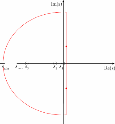
Figure 3: (color online). Contour of integration (red line) chosen to calculate inverse Laplace transform Eq. (58). Points of nonanalytic behavior of $\sigma_{{}_{\textrm{++}}}(s)$ are shown. (Poles at $s_{1}$, $s_{2}$, and $s_{3}$, and a cut $s\in(s_{\rm{min}},s_{\rm{max}})$).

In the slow relaxation case, $\Gamma_{\textrm{in}}\tau\gg 1$, the main contribution to the integral (58) comes from the cut, and poles $s_{1}=0$ and $s_{2}$. The latter may be found by iterative solution of Eq. (59),

$$s_{2}=-\frac{Z(0)}{\tau}\left(1\!+\!e^{-E_{{}_{J}}/T}\right),$$

where function $Z(0)$ is defined in Eq. (56), and in the case of slow relaxation can be approximated as

$$Z(0)=\frac{1}{\delta_{r}}\int_{\Delta}^{\infty}dE_{p}\nu(E_{p})\frac{\gamma_{{}_{+}}(E_{p})}{\Gamma(E_{p})}\rho_{\rm{odd}}(E_{p}).$$ (61)

The residue at $s_{3}$ gives a smaller by factor $1/\Gamma_{\textrm{in}}\tau\ll 1$ contribution, see the Appendix.

Taking integral in Eq. (58) along the contour enclosing the cut shown in Fig. 3, and accounting for poles $s_{1}$ and $s_{2}$, we find

$$\!\sigma_{{}_{++}}\!(t)\!\! \!\!=\!\! \!\!\frac{e^{-\!E_{{}_{J}}/T}}{1\!+\!e^{-\!E_{{}_{J}}/T}}\!+\!\left(\!\frac{1}{1\!+\!e^{-\!E_{{}_{J}}/T}}\!-\!Z(0)\!\right)\!\times\!$$

$$\!\times\! \!\exp\!\left(\!-Z(0)\!\left(1\!+\!e^{-\!E_{{}_{J}}/T}\right)\frac{t}{\tau}\!\right)\!+\!$$

$$\!+\! \!\!\frac{1}{\delta_{r}}\int_{\Delta}^{\infty}dE_{p}\nu(E_{p})\frac{\gamma_{{}_{+}}(\!E_{p})\rho_{\rm{odd}}(\!E_{p})}{\Gamma(E_{p})}\exp\!\left(\!-\Gamma(E_{p})\,t\right).$$

Here we neglected the corrections to Eq. (VI.2) of the order $1/\Gamma_{\textrm{in}}\tau$. The obtained expression for $\!\sigma_{{}_{++}}\!(t)$ describes the kinetics of the qubit populations in the slow relaxation regime. Note that the solution Eq. (VI.2) satisfies initial conditions $\sigma_{{}_{++}}(0)=1$ and is consistent with previous results. Indeed, in the limit $\tau\!\rightarrow\!\infty$, the exponent in the second term goes to zero and we recover Eq. (V) (To show this one should use Eq. (34)).

Equation (VI.2) becomes physically transparent in the low-temperature limit. Using the approximation (38) for $Z(0)$ and for the integral in the last term of Eq. (VI.2) we find

$$\!\sigma_{{}_{++}}(t)\! \!=\! \!\frac{e^{-E_{{}_{J}}/T}}{1\!+\!e^{-E_{{}_{J}}/T}}\!+\!\sqrt{\frac{T}{\pi E_{{}_{J}}}}\exp\left(\!-\frac{t}{T_{1}^{*}}\right)$$ (63)

$$\!+\! \!\left(\frac{1}{1\!+\!e^{-E_{{}_{J}}/T}}\!-\!\sqrt{\frac{T}{\frac{}{}\pi E_{{}_{J}}}}\,\right)\!\exp\!\left(-\!\frac{t}{T_{1}}\right),$$

where relaxation times $T_{1}$ and $T_{1}^{*}$ are

$$\frac{1}{T_{1}}\!=\!\frac{1}{\tau}\sqrt{\frac{T}{\pi E_{{}_{J}}}}\mbox{ and }\frac{1}{T_{1}^{*}}\!=\!\frac{g_{{}_{T}}\delta_{r}}{4\pi}\sqrt{\frac{\omega_{{}_{+}}}{2\Delta+\omega_{{}_{+}}}}\left(1\!+\!\frac{E_{{}_{J}}}{\omega_{{}_{+}}}\right).$$ (64)

Obtained results describe the relaxation of the qubit populations in the slow relaxation limit ($\Gamma_{\textrm{in}}\tau\gg 1$) discussed qualitatively in Sec. II. According to Eq. (63), in this case the process of equilibration of qubit populations occurs in two stages. The first stage ($t\sim T_{1}^{*}$) corresponds to a quasistationary state formation with qubit populations much larger than equilibrium ones. For the typical experimental temperatures $T\!\sim\!20$ mK, the excited state population of the qubit is about $85\%$. The equilibrium populations are established in the second stage, on the time scale of $T_{1}$. The relaxation time $T_{1}$ sets an important experimental constraint on the frequency of repetition of qubit experiments.

We estimate now energy and phase relaxation times for the realistic experimental parameters Nakamura ; Wallraff : $\Delta\!\approx\!2K$, $E_{c}\!\approx\!0.5K$, $E_{{}_{J}}\!\approx\!0.3K$, $g_{{}_{T}}\!\sim\!1$, and $T\!\approx\!20mK$. For the volume of the reservoir $10^{-19}-10^{-17}m^{3}$, Eq. (29) yields the phase relaxation time $T_{2}\sim 10^{-5}\!-\!10^{-3}s$. Energy relaxation depends on the relation between $\Gamma_{in}$ and $1/\tau$. Taking $\tau\!\sim\!10^{-4}s$ and $\Gamma_{in}^{-1}\!\sim\!10^{-5}s$, which corresponds to the lower end of the volume range, energy relaxation is described by Eq. (63) with $T_{1}^{*}\!\sim\!10^{-5}s$ and $T_{1}\!\sim\!10^{-3}s$.

We considered so far the effect of a single quasiparticle on the qubit kinetics. It is possible to generalize our results onto the case of many quasiparticles $N_{\textrm{qp}}$ residing in the system. In this case $T_{2}$ becomes shorter since the quasiparticle tunneling rate $\Gamma_{\textrm{in}}$, see Eq. (3), should be multiplied by the number of quasiparticles in the superconducting reservoir

$$\frac{1}{T_{2}}\simeq\Gamma_{\textrm{in}}\cdot N_{\textrm{qp}}\simeq\frac{g_{{}_{\textrm{T}}}n_{\textrm{qp}}}{4\pi\nu}.$$ (65)

(Here $\nu$ is the normal density of states per unit volume and $n_{\rm qp}$ is the density of quasiparticles in the reservoir.) Note that the volume of the reservoir does not enter in Eq. (65). A finite density of quasiparticles in the reservoir affects also the process of energy relaxation of the qubit. The most clear example corresponds to the limit $\Gamma_{\rm in}\tau\ll\!~{}\!1$ in which quasiparticle relaxation in the reservoir occurs fast compared to the time needed for the quasiparticle to reenter the CPB. In this limit $T_{1}/T_{2}\sim\sqrt{E_{J}/T}$.

The comparison of the theoretical prediction for $T_{2}$ and $T_{1}$ with experimental data is complicated by the unknown value of $N_{\rm qp}$ in a qubit. The quasiparticle density in a system with a massive lead is known to deviate from the equilibrium value in a number of experiments Prober ; Aumentado . The estimate of $n_{\rm qp}$ can be obtained from the kinetics of “quasiparticle poisoning” studied in the recent experiments Naaman ; Schneiderman . The observed rate of quasiparticle entering the CPB was $10^{5}-10^{4}$ Hz. Assuming that the bottleneck for the quasiparticles was tunneling through the junction (rather than the diffusion in the lead), we estimate the density of quasiparticles in the lead to be $n_{\textrm{qp}}\sim 10^{19}-10^{18}\,\textrm{m}^{-3}$. The same quasiparticle density in a qubit with the reservoir volume $10^{-19}-10^{-17}m^{3}$ would result in $N_{\textrm{qp}}\sim 1-100$.

VII Conclusions

We studied the kinetics of a superconducting charge qubit in the presence of an unpaired electron. The presence of a quasiparticle in the system leads to the decay of quantum oscillations. We obtained master equations for the coherences and populations of the qubit, which take into account energy exchange between the quasiparticle and the qubit, and include the mechanisms of quasiparticle relaxation due to electron-phonon interaction. Finally, we found decay exponents governing the dynamics of the qubit for different cases: fast and slow quasiparticle relaxation in the reservoir.

We have shown that phase relaxation is determined by the quasiparticle tunneling rate to the box $\Gamma_{\textrm{in}}\sim g_{{}_{T}}\delta_{r}/4\pi$. Kinetics of the qubit populations depends on the ratio of the quasiparticle relaxation time $\tau$ and escape time $\Gamma_{\textrm{in}}^{-1}$. In this paper, we considered two limits - fast ($\tau\Gamma_{\textrm{in}}\ll 1$) and slow ($\tau\Gamma_{\textrm{in}}\gg 1$) quasiparticle relaxation. In the latter case, decay of qubit populations occurs in two stages. In the first stage at $t\sim\Gamma_{\textrm{in}}^{-1}$ a quasistationary regime is established with large nonequilibrium excited state population. The second stage describes the attainment of the equilibrium populations and occurs on the time scale of $\tau\sqrt{\pi E_{{}_{J}}/T}$. In the fast relaxation case, equilibrium qubit populations are established at $t\sim\Gamma_{\textrm{in}}^{-1}\sqrt{\pi E_{{}_{J}}/T}$.

Appendix A Analysis of the analytical structure of $\sigma_{{}_{\textrm{++}}}(s)$.

In this appendix we study the analytic properties of $\sigma_{{}_{\textrm{++}}}(s)$ in order to calculate the inverse Laplace transform (58). In general, the nonanalytic behavior of $\sigma_{{}_{\textrm{++}}}(s)$ is determined by three poles, one of them is at $s=0$, and a cut as shown in Fig. 3. The locations of two other poles and of the cut, and also contributions of all the mentioned singularities in $\sigma_{{}_{\textrm{++}}}(s)$ to the integral (58), depend on the value of $\Gamma_{\textrm{in}}\tau$.

In the fast relaxation regime ($\Gamma_{\textrm{in}}\tau\ll 1$), in the vicinity of the $s=0$ pole, we find

$$\sigma_{{}_{\textrm{++}}}(s)=\frac{e^{-E_{{}_{J}}/T}}{1+e^{-E_{{}_{J}}/T}}\frac{1}{s}.$$ (66)

Two other poles $s_{2}$ and $s_{3}$ are the solutions of Eq. (59) with $s_{2}$ being the solution at small $s\sim\Gamma_{\textrm{in}}$ and $s_{3}$ at large $s\sim 1/\tau$:

$$s_{2} = -\left(\left<\!\gamma_{{}_{+}}\!\right>+\left<\!\gamma_{{}_{-}}\!\right>\right),$$

$$s_{3} = -\frac{1}{\tau}-\mbox{\rm min}\left[\,\Gamma(E_{p})\,\right]+\frac{g_{{}_{T}}\delta_{r}}{4\pi}C_{1}.$$ (67)

Here $\Gamma(E_{p})$ is defined in Eq. (37) and $C_{1}$ is a distance from the beginning of the cut in units of $g_{{}_{T}}\delta_{r}/4\pi$, see Fig. 3. In the vicinity of the second pole, $\sigma_{{}_{\textrm{++}}}(s)$ is given by

$$\sigma_{{}_{\textrm{++}}}(s)=\left(\frac{1}{1+e^{-E_{{}_{J}}/T}}-Z(0)\right)\frac{1}{s-s_{2}},$$ (68)

with $Z(0)$ defined in Eq. (61). The residue of $\sigma_{{}_{\textrm{++}}}(s)$ at $s_{3}$ is proportional to $(\tau\Gamma_{\textrm{in}})^{2}$. Consequently, the contribution to the integral (58) from the pole $s_{3}$ is small.

In addition to the poles discussed above, nonanalyticity of $\sigma_{{}_{\textrm{++}}}(s)$ comes from the singularities of $Z(s)$. The function $Z(s)$ is nonanalytic along the cut $s\in\left(s_{\rm min},s_{\rm max}\right)$, where

$$s_{\rm min}\! \!=\! \!-\frac{1}{\tau}\!-\!\mbox{\rm max}\left[\Gamma(E_{p})\right],$$

$$s_{\rm max}\! \!=\! \!-\!\frac{1}{\tau}\!-\!\mbox{\rm min}\left[\Gamma(E_{p})\right],$$

with $\Gamma(E_{p})$ being defined in Eq. (37). The proper contribution to Eq. (58) can be calculated by integrating along the contour enclosing the cut

$$\!I_{\rm cut}\! \!=\! \!\frac{\!-\!1}{2\pi i}\int_{s_{\rm min}}^{s_{\rm max}}{ds}e^{st}\left(\sigma_{{}_{\textrm{++}}}(s\!+\!i\epsilon)\!-\!\sigma_{{}_{\textrm{++}}}(s\!-\!i\epsilon)\right).$$

The discontinuity of the imaginary part of $\sigma_{{}_{\textrm{++}}}(s)$ at the cut is

$$\sigma_{{}_{\textrm{++}}}(s\!+\!i\epsilon)\!-\!\sigma_{{}_{\textrm{++}}}(s\!-\!i\epsilon)=$$

$$\!=\! \!\frac{-2i\tau(\tau s\!+\!1)\mbox{\rm Im}Z(s\!+\!i\epsilon)}{[\tau s\!+\!\mbox{\rm Re}Z(s)(1\!+\!e^{\!-\!E_{{}_{J}}/T})]^{2}\!+\![\mbox{\rm Im}Z(\!s\!+\!i\epsilon\!)(1\!+\!e^{\!-\!E_{{}_{J}}/T})]^{2}}.$$

In the limit $\Gamma_{\textrm{in}}\tau\ll 1$ we find

$$\sigma_{{}_{\textrm{++}}}(s\!+\!i\epsilon)\!-\!\sigma_{{}_{\textrm{++}}}(s\!-\!i\epsilon)\! \!\approx\! \!\frac{-2i\tau(\tau\Gamma_{\textrm{in}})\mbox{\rm Im}Z(s\!+\!i\epsilon)}{[\!-\!1\!+\!\mbox{\rm Re}Z(s)]^{2}\!+\![\mbox{\rm Im}Z(\!s\!+\!i\epsilon\!)]^{2}},$$

which yields a negligible contribution to Eq. (58) from the cut, $I_{cut}\propto\Gamma_{\textrm{in}}\tau\ll 1$. Finally, after summing up two relevant contributions, one obtains the result for $\sigma_{{}_{\textrm{++}}}(t)$ given in Eq. (VI.1).

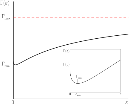
Figure 4: (color online) Main panel: dependence of $\Gamma(\varepsilon)$, defined in Eq. (37), on quasiparticle energy $\varepsilon=E_{p}-\Delta$. Inset: dependence of $\Gamma(\varepsilon)$ in the vicinity of $\varepsilon_{{}_{\rm min}}$. The maximum value of the rate is $\Gamma_{\rm max}=g_{{}_{T}}\delta_{r}/4\pi$ (dashed line). In the limit $E_{{}_{J}}\ll\omega_{{}_{+}}\ll\Delta$, a simple analytic expression for the minimum can be found: $\varepsilon_{{}_{\rm min}}=E_{{}_{J}}/25$, and $\frac{\Gamma_{\rm{min}}-\Gamma(0)}{\Gamma(0)}\approx-C\frac{E_{{}_{J}}}{\omega_{{}_{+}}}$, where $\Gamma(0)=\frac{g\delta_{r}}{4\pi}\sqrt{\frac{\omega_{{}_{+}}}{2\Delta}}$, and numerical constant $C\approx 0.1$.

In the opposite limit of slow relaxation ($\Gamma_{\textrm{in}}\tau\gg 1$), the first pole $s_{1}=0$ is the same as in the previous case with the expression for $\sigma_{{}_{\textrm{++}}}(s)$ given by Eq. (66). The other two poles $s_{2}$ and $s_{3}$ are found from Eq. (59) assuming $\Gamma_{\textrm{in}}\tau\gg 1$:

$$s_{2} = -\frac{Z(0)}{\tau}\left(1\!+\!e^{-E_{{}_{J}}/T}\right),$$

$$s_{3} = \!-\mbox{min}[\,\Gamma(E_{p})\,]\!-\frac{1}{\tau}+\frac{C_{2}}{\tau^{2}\Gamma_{\textrm{in}}},$$ (72)

where $Z(0)$ is defined in Eq. (61), and $C_{2}$ is a positive constant of the order of unity. In the vicinity of the second pole $\sigma_{{}_{\textrm{++}}}(s)$ is given by

$$\sigma_{{}_{\textrm{++}}}(s)=\left(\frac{1}{1+e^{-E_{{}_{J}}/T}}-Z(0)\right)\frac{1}{s-s_{2}}.$$ (73)

The third pole $s_{3}$ lies in close proximity to the beginning of the cut $s_{{\rm max}}$. In order to find the position of the pole we expand the denominator of $Z(s)$ in the neighborhood of the minimum of $\Gamma(E_{p})$, see Fig. 4:

$$Z(s)\!=\!\int_{\Delta}^{\infty}{\frac{dE_{p}}{\delta_{r}}}\frac{\nu(E_{p})\gamma_{{}_{+}}(E_{p})\rho_{\rm{odd}}(E_{p})}{s\!+\!1/\tau\!+\!\Gamma_{\rm min}\!+\!\Gamma^{\prime\prime}(E{{}_{p}}_{\rm min})(E_{p}\!-\!E{{}_{p}}_{\rm min})^{2}},$$

and solve Eq. (59) to obtain $s_{3}$ of Eq. (A). Here we used the small-$y$ asymptote, $Z(y)\propto 1/\sqrt{y}$, where $y$ is the distance from $s_{\rm max}$ in units of $\Gamma_{\textrm{in}}$; i.e., we made a substitution

$$s=-1/\tau-\Gamma_{\rm min}+\Gamma_{\textrm{in}}y$$

in Eq. (A) and evaluated the integral at $y\ll 1$. Then, in the neighborhood of $s_{3}$ the expression for $\sigma_{{}_{\textrm{++}}}(s)$ can be written as

$$\sigma_{{}_{\textrm{++}}}(s)\approx\frac{\Gamma_{\textrm{in}}\tau Z(y_{0})}{\Gamma_{\textrm{in}}\tau+Z^{\prime}(y_{0})(1+e^{-E_{{}_{J}}/T})}\frac{1}{s-s_{3}},$$ (75)

where $y_{0}$ is the corresponding solution of Eq. (59) and is small: $y_{0}\!\sim\!(\Gamma_{\textrm{in}}\tau)^{-2}\ll 1$. Since derivative $Z^{\prime}(y_{0})\propto y_{0}^{-3/2}$, the residue at $s_{3}$ is suppressed as $(\Gamma_{\textrm{in}}\tau)^{-1}$ and thus can be neglected.

The contribution from the cut in the limit $\Gamma_{\textrm{in}}\tau\gg 1$ can be evaluated from Eq. (A). The discontinuity of the function $\sigma_{{}_{\textrm{++}}}(s)$ is

$$\sigma_{{}_{\textrm{++}}}(s\!+\!i\epsilon)\!-\!\sigma_{{}_{\textrm{++}}}(s\!-\!i\epsilon)\approx-\frac{2i}{s}\mbox{\rm Im}Z(s\!+\!i\epsilon).$$ (76)

Hence, the contribution to Eq. (58) from the cut is

$$\!I_{\rm cut}\! \!=\! \!-\!\int_{\Delta}^{\infty}\!\frac{dE_{p}}{\delta_{r}}\nu(E_{p})\!\gamma_{{}_{+}}\!(\!E_{p})\!\rho_{\rm{odd}}(\!E_{p})\!\int_{\!s_{\rm min}\!}^{\!s_{\rm max}\!}{\!ds}\!\frac{e^{st}}{s}\delta\!\left(\!s\!+\Gamma(E_{p})\right)$$ (77)

$$\!=\! \!\int_{\Delta}^{\infty}\frac{dE_{p}}{\delta_{r}}\nu(E_{p})\frac{\gamma_{{}_{+}}(E_{p})\rho_{\rm{odd}}(E_{p})}{\Gamma(E_{p})}\exp\left(-\Gamma(E_{p})t\right).$$

Finally, combining proper terms one finds the inverse Laplace transform of Eq. (VI.2).

References

- (1) Y. Nakamura, Y. A. Pashkin, and J. S. Tsai, Nature 398, 786 (1999)
- (2) A. Wallraff, D. I. Schuster, A. Blais, L. Frunzio, R.-S. Huang, J. Majer, S. Kumar, S. M. Girvin and R. J. Schoelkopf, Nature (London) 431, 162 (2004).
- (3) D. Vion, A. Aassime, A. Cottet, P. Joyez, H. Pothier, C. Urbina, D. Esteve, and M.H. Devoret, Science 296, 286 (2002).
- (4) A. Blais, R.-S. Huang, A. Wallraff, S. M. Girvin, R. J. Schoelkopf, Phys. Rev. A 69, 062320 (2004)
- (5) D. DiVincenzo, Fortschr. Phys. 48, 771 (2000)
- (6) M. H. Devoret, A. Wallraff, J. M. Martinis, cond-mat/0411174
- (7) O. Astafiev, Yu. A. Pashkin, Y. Nakamura, T. Yamamoto, and J. S. Tsai, Phys. Rev. Lett. 93, 267007 (2004)
- (8) R. Lutchyn, L. Glazman, A. Larkin, Phys. Rev. B 72, 014517 (2005)
- (9) Y. Makhlin, G. Schön, A. Shnirman, Rev. Mod. Phys. 73, 357 (2001)
- (10) A. Guillaume, J. F. Schneiderman, P. Delsing, H. M. Bozler, and P. M. Echternach, Phys. Rev. B 69, 132504 (2004)
- (11) Ya.M. Blanter, V.M. Vinokur, and L.I. Glazman, cond-mat/0504309
- (12) The possibility to include the Josephson tunneling term in while considering the quasiparticle tunneling Hamiltonian as a perturbation was demonstrated in Ref. [8].
- (13) S.B. Kaplan et. al., Phys. Rev. B 14, 4854 (1976)
- (14) C.C. Chi and J. Clarke, Phys. Rev. B 19, 4495 (1979)
- (15) D. Zubarev, V. Morozov and G. Röpke, Statistical Mechanics of Nonequilibrium Processes, (Akademie Verlag, Berlin, 1996).
- (16) M. Esposito and P. Gaspard, Phys. Rev. E 68, 66112 (2003).
- (17) J.R. Schrieffer, Theory of Superconductivity, (Oxford : Advanced Book Program, Perseus, 1999).
- (18) M. Tinkham, Introduction to Superconductivity, (McGraw-Hill, New York, 1996), p. 81.
- (19) We do not consider here qubit relaxation originating from the excitation of phonons by charge fluctuations across the Josephson junction Ioffe . The presence of a quasiparticle opens a relaxation channel that is faster than the mechanism considered in Ref. [20].
- (20) L. B. Ioffe, V. B. Geshkenbein, C. Helm, and G. Blatter, Phys. Rev. Lett. 93, 057001 (2004).
- (21) C. M. Wilson and D. E. Prober, Phys. Rev. B 69, 094524 (2004)
- (22) J. Aumentado, M. W. Keller, J. M. Martinis, M. H. Devoret, Phys. Rev. Lett. 92, 66802 (2004).
- (23) O. Naaman and J. Aumentado, Phys. Rev. B 73, 172504 (2006)
- (24) J.F. Schneiderman, P. Delsing, G. Johansson, M.D. Shaw, H.M. Bozler, and P.M. Echternach, unpublished.