Angle-resolved photoemission spectroscopy of perovskite-type transition-metal oxides and their analyses using tight-binding band structure

Abstract

Nowadays it has become feasible to perform angle-resolved photoemission spectroscopy (ARPES) measurements of transition-metal oxides with three-dimensional perovskite structures owing to the availability of high-quality single crystals of bulk and epitaxial thin films. In this article, we review recent experimental results and interpretation of ARPES data using empirical tight-binding band-structure calculations. Results are presented for SrVO₃ (SVO) bulk single crystals, and La_1-xSr_xFeO₃ (LSFO) and La_1-xSr_xMnO₃ (LSMO) thin films. In the case of SVO, from comparison of the experimental results with calculated surface electronic structure, we concluded that the obtained band dispersions reflect the bulk electronic structure. The experimental band structures of LSFO and LSMO were analyzed assuming the G-type antiferromagnetic state and the ferromagnetic state, respectively. We also demonstrated that the intrinsic uncertainty of the electron momentum perpendicular to the crystal surface is important for the interpretation of the ARPES results of three-dimensional materials.

I Introduction

Perovskite-type $3d$ transition-metal (TM) oxides have been attracting much interest in these decades because of their intriguing physical properties, such as metal-insulator transition (MIT), colossal magnetoresistance (CMR), and ordering of spin, charge, and orbitals rev . Early photoemission studies combined with cluster-model analyses have revealed that their global electronic structure is characterized by the TM $3d$-$3d$ on-site Coulomb interaction energy denoted by $U$, the charge-transfer energy from the occupied O $2p$ orbitals to the empty TM $3d$ orbitals denoted by $\Delta$, and the $p$-$d$ hybridization strength denoted by $(pd\sigma)$ ZSA . If $\Delta>U$, the band gap is of the $d$-$d$ type, and the compound is called a Mott-Hubbard-type insulator. For $\Delta<U$, the band gap is of the $p$-$d$ type: the O $2p$ band is located between the upper and lower Hubbard bands, and the compound is called a charge-transfer-type insulator. In going from lighter to heavier $3d$ TM elements, the $d$ level is lowered and therefore $\Delta$ is decreased, whereas $U$ is increased. Thus Ti and V oxides become Mott-Hubbard-type compounds and Mn, Fe, Co, Ni, and Cu oxides charge-transfer-type compounds.

Having established the global electronic structure picture of the transition-metal oxides with their chemical trend, the next step is to understand the momentum dependence of the electronic states, that is, the “band structure” of the hybridized $p$-$d$ states influenced by the Coulomb interaction $U$. Angle-resolved photoemission spectroscopy (ARPES) is a unique and most powerful experimental technique by which one can directly determine the band structure of a material. However, ARPES studies have been largely limited to low-dimensional materials and there have been few studies on three-dimensional TM oxides with cubic perovskite structures because many of them do not have a cleavage plane. Recently, Yoshida et al. succeeded in cleaving single crystals of SrVO₃ (SVO) along the cubic $(100)$ surface and performed ARPES measurements SVOARPES . Another way of performing ARPES studies of such materials is the use of single-crystal thin films. Recently, high-quality perovskite-type oxide single-crystal thin films grown by the pulsed laser deposition (PLD) method have become available Izumi ; Choi , and setups have been developed for their in-situ photoemission measurement Horiba ; Shi . By using well-defined surfaces of epitaxial thin films, we recently studied the band structures of La_1-xSr_xFeO₃ (LSFO) and La_1-xSr_xMnO₃ (LSMO), and it has been demonstrated that in-situ ARPES measurements on such TM oxide films are one of the best methods to investigate the band structure of TM oxides with three-dimensional crystal structures Chika ; LSFOARPES .

In this paper, we report on analyses of ARPES results of bulk single crystals of SVO SVOARPES and on in-situ ARPES results of single-crystal LSFO ($x=0.4$) LSFOARPES and LSMO ($x=0.4$) Chika thin films grown on SrTiO₃ (001) substrates. In the case of SVO, we have investigated the effect of surface on the ARPES spectra by comparing the experimental results with calculated surface electronic structures. The experimental band structures of LSFO and LSMO were interpreted using an empirical tight-binding band-structure calculation by assuming the G-type antiferromagnetic state for LSFO and the ferromagnetic state for LSMO. The mass enhancement compared with band-structure calculation is discussed in the case of SVO and LSMO. We also discuss the problem of intrinsic uncertainty in determining the momentum of electrons in the solid perpendicular to the crystal surface 3DARPES .

II Theoretical analyses

II.1 Tight-binding band-structure calculation

In the case of SVO, we adopted the simplest tight-binding (TB) model. In this simplest model, the $t_{2g}$ bands are represented by a TB Hamiltonian with diagonal elements of the form

$$H_{xy,xy}(\mbox{\boldmath$k$}) = e_{d}+t_{0}(c_{x}+c_{y})+t_{1}c_{x}c_{y}+[t_{2}+t_{3}(c_{x}+c_{y})+t_{4}c_{x}c_{y}]c_{z},$$ (1)

where $c_{i}=2\cos(k_{i}a)$ ($i=x$, $y$, $z$) and $a$ is the lattice constant Liebsch . Cyclic permutations yield $H_{yz,yz}(\mbox{\boldmath$k$})$ and $H_{zx,zx}(\mbox{\boldmath$k$})$. The $t_{i}$ denote effective hopping integrals arising from the V-O-V hybridization. $t_{0,2}$, $t_{1,3}$, and $t_{4}$ specify the interaction between first, second, and third neighbors, respectively, and $|t_{0}|\gg|t_{1}|$, $|t_{2}|$, $|t_{3}|$, $|t_{4}|$. Off-diagonal elements which vanish at high-symmetry points are small and are neglected here.

In the case of LSFO and LSMO, we performed TB band-structure calculations explicitly including oxygen $2p$ orbitals for the three-dimensional perovskite structure in the antiferromagnetic (AF) and ferromagnetic (FM) states. TB calculations for the paramagnetic (PM) state were already reported in Refs. Kahn ; ReO3 ; STO . The size of the matrix for the latter calculation was $14\times 14$ (TM $3d$ orbitals: 5, oxygen $2p$ orbitals: $3\times 3=9$). As for LSFO, we performed the calculation assuming the G-type AF state, where all nearest-neighbor Fe atoms have antiparallel spins. The effect of the G-type antiferromagnetism was treated phenomenologically by assuming an energy difference $\Delta E$ between the spin-up and spin-down Fe sites. As for LSMO, we performed the calculation assuming the FM state. The effect of ferromagnetism was again treated phenomenologically by assuming an energy difference $\Delta E$ between the spin-up and spin-down Mn sites. The size of the matrix to be diagonalized was $28\times 28$ for LSFO (G-type AF), and $14\times 14$ for LSMO (FM). Parameters to be adjusted are $\Delta E$, the energy difference between the TM $3d$ level and the O $2p$ level $\epsilon_{d}-\epsilon_{p}$, and Slater-Koster parameters $(pd\sigma)$, $(pd\pi)$, $(pp\sigma)$, and $(pp\pi)$ JC . Here, $\epsilon_{d}$ is the average of the majority-spin $d$-level $\epsilon_{d}-\Delta E/2$ and the minority-spin $d$-level $\epsilon_{d}+\Delta E/2$. The ratio $(pd\sigma)/(pd\pi)$ was fixed at $-2.2$ WA ; STO1 , and $(pp\sigma)$ and $(pp\pi)$ were fixed at $0.60$ eV and $-0.15$ eV, respectively. $(pd\sigma)$ is expected to be in the range of $-(1.4-1.9)$ eV for LSFO and near $-1.8$ eV for LSMO from a configuration-interaction (CI) cluster-model calculation reported in Refs. Bocquet2 ; Wadati . Crystal-field splitting $10Dq$ of 0.41 eV was taken from Ref. Wadati . Crystal-field splitting of O $2p$ orbitals is not taken into account. The TB basis functions used in the calculations of LSFO and LSMO are given in Tables LABEL:symbol1 and LABEL:symbol3, and the matrix elements of the Hamiltonians for LSFO and LSMO are given in Tables LABEL:symbol2 and LABEL:symbol4, respectively.

Figure 1 shows the Brillouin zones (BZs) for the perovskite structure in the PM and FM states [(a)], the G-type AF state [(b)], and the G-type AF state with GdFeO₃-type distortion [(c)]. The BZ of the FM state is the same as that of the PM state. The BZ of the G-type AF state is that of the face-centered cubic (fcc) lattice. In this paper, we will neglect the effect of the GdFeO₃-type distortion and will only consider the effect of magnetic ordering.

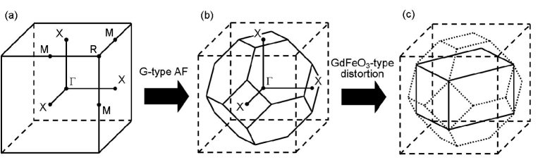
Figure 1: Brillouin zones of the perovskite structure. (a)PM and FM states. (b)G-type AF state. Broken lines represent the BZ of the PM state. (c)G-type AF state with GdFeO₃-type distortion. Broken lines and dotted lines represent the BZs of the PM state and the G-type AF state, respectively.

Figure 2 shows schematic band structures along the $\Gamma$-X line obtained by TB calculation. Here, we have fixed $\epsilon_{d}-\epsilon_{p}-\Delta E/2$ at 3 eV. Panel (a) shows the band structure of the PM state calculated including only $p$-$p$ interactions, namely, without $p$-$d$ interaction ($(pd\sigma)=0$). There are significant dispersions in the O $2p$ bands caused by the $p$-$p$ interaction, whereas there are no dispersions in the $e_{g}$ and $t_{2g}$ bands, where there exists only the crystal-field splitting of $10Dq$. Panel (b) shows the band structure of the PM state calculated with $(pd\sigma)=-2.0$ eV. The $e_{g}$ and $t_{2g}$ bands now become dispersive due to the $p$-$d$ interaction. Panels (c) and (d) show the band structure of the FM and G-type AF states, respectively. The values of $\Delta E$ were taken as 5.0 eV in both cases. In the FM state, since $\epsilon_{d}-\epsilon_{p}-\Delta E/2$ is fixed, the up-spin (majority-spin) $e_{g}$ and $t_{2g}$ bands do not change appreciably compared with those in the PM state, whereas the down-spin (minority-spin) $e_{g}$ and $t_{2g}$bands are pushed up by $\Delta E$ (out of the range of Fig. 2 (c)). In the G-type AF state, band dispersions along the R-M line are folded onto the $\Gamma$-X line, and hybridization between these bands causes a maximum in the $e_{g}$ bands in the middle of $\Gamma$ and X.

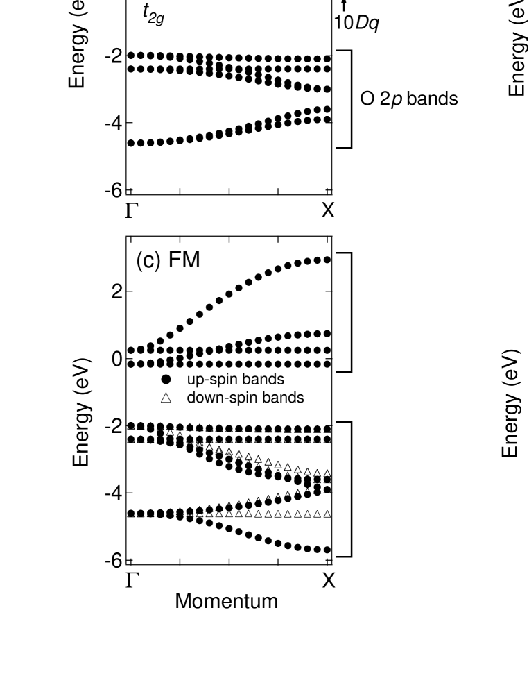
Figure 2: Band structures obtained by TB calculation. $\epsilon_{d}-\epsilon_{p}-\Delta E/2=3$ eV has been fixed. (a)PM state with only $p$-$p$ interaction included ($(pd\sigma)=0$). (b)PM state with $(pd\sigma)=-2.0$ eV. (c)FM state with $\Delta E=5.0$ eV. (d)G-type AF state with $\Delta E=5.0$ eV.

II.2 $k_{z}$ broadening

In ARPES measurements, there is an intrinsic uncertainty in the momentum of electrons in the solid perpendicular to the crystal surface due to a finite escape depth $\lambda$ of photoelectrons 3DARPES . Here, the $z$-axis is taken as the direction perpendicular to the surface toward the vacuum side. Inside the solid ($z<0$) the wave function of an emitted photoelectron with a wave number $k_{z0}$ is approximated by

$$\psi(z)=\frac{1}{\sqrt{\lambda}}\exp(ik_{z0}z)\exp(z/2\lambda),$$ (2)

where $\lambda$ denotes the escape depth of a photoelectron. $|\psi(z)|^{2}=\exp(z/\lambda)/\lambda$ shows an exponential decay of photoelectrons within the solid. The Fourier transform of Eq. (2), $\phi(k_{z})$, is

$$\phi(k_{z})\propto\frac{1}{i(k_{z}-k_{z0})-1/2\lambda}.$$ (3)

and $|\phi(k_{z})|^{2}$ becomes proportional to

$$L(k_{z})=\frac{1}{2\pi\lambda}\frac{1}{(k_{z}-k_{z0})^{2}+(1/2\lambda)^{2}},$$ (4)

which means that the intrinsic uncertainty of $k_{z}$ is given by the Lorentzian function with the full width at half maximum of $1/\lambda$.

The effect of the $k_{z}$ broadening is very important for the interpretation of ARPES results. For example, we consider an isotropic band with the bottom at the $\Gamma$ point, expressed as

$$E=\alpha(k_{x}^{2}+k_{y}^{2}+k_{z}^{2}).$$ (5)

If we measure photoelectrons with momentum $\overrightarrow{K}=(K_{x}.K_{y},K_{z})$, where $K_{z}$ is related to $k_{z0}$ through the momentum conservation $k_{x}=K_{x}$ and $k_{y}=K_{y}$ and the energy conservation, the obtained spectrum becomes,

$$D(k_{x},k_{y},E)=\displaystyle\int^{\infty}_{-\infty}dk_{z}L(k_{z})\delta(E-\alpha({k_{x}}^{2}+{k_{y}}^{2}+{k_{z}}^{2})).$$ (6)

From Eq. (4) and using the identity

$$\delta(x-\alpha{k_{z}}^{2})=\frac{1}{2\sqrt{\alpha x}}\left[\delta\left(k_{z}-\sqrt{\frac{x}{\alpha}}\right)+\delta\left(k_{z}+\sqrt{\frac{x}{\alpha}}\right)\right],$$ (7)

we obtain

$$\begin{array}[]{c}D(k_{x},k_{y},E)=\displaystyle\frac{1}{4\pi\lambda\sqrt{\alpha\{E-\alpha({k_{x}}^{2}+{k_{y}}^{2})\}}}\times\\ \left[\displaystyle\frac{1}{\left(\sqrt{\{E-\alpha({k_{x}}^{2}+{k_{y}}^{2})\}/\alpha}-k_{z0}\right)^{2}+(1/2\lambda)^{2}}\right.\\ +\left.\displaystyle\frac{1}{\left(\sqrt{\{E-\alpha({k_{x}}^{2}+{k_{y}}^{2})\}/\alpha}+k_{z0}\right)^{2}+(1/2\lambda)^{2}}\right].\end{array}$$ (8)

We plot the function $D(k_{x},k_{y},E)$ with $k_{x}=k_{y}=0$ for various values of $\lambda$ in Fig. 3. Here, we have assumed that $\alpha=8$ eV$\cdot\mbox{\AA}^{2}$, which corresponds to $m^{\ast}\sim 0.5m_{e}$ ($m^{\ast}$ is an effective band mass and $m_{e}$ is the electron mass in vacuum), and $k_{z0}=\pi/4c$, where $c=3.830\ \mbox{\AA}$, the out-of-plane lattice constant of LSMO ($x=0.4$) thin films. One can see that in bulk-sensitive measurements using high-energy photons, like $\lambda=20\ \mbox{\AA}$, there is a peak at $E=\alpha{k_{z0}}^{2}$. In contrast, in surface-sensitive measurements using low-energy photons, there is no peak at $\alpha{k_{z0}}^{2}$ but $D(E)$ is peaked around $E\sim 0$. The density of states at the $\Gamma$ point is very large because the band has a van Hove singularity at this point. Since bands usually have van Hove singularities along a high-symmetry line, the effect of $k_{z}$ broadening is very important when we trace near the high-symmetry line using low energy photons. Our photon energies used in the ARPES measurements were in the range of $20-100$ eV and therefore $\lambda\sim 5\mbox{\AA}$, meaning that considering the $k_{z}$-broadening effect is crucial in the interpretation of ARPES results.

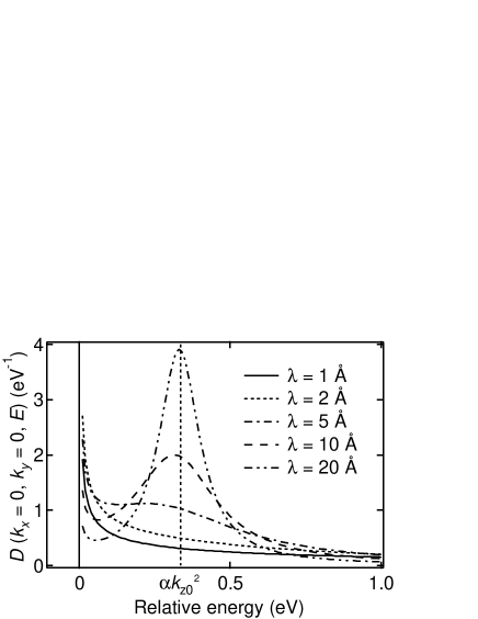
Figure 3: ARPES spectrum $D(k_{x},k_{y},E)$ with $k_{x}=k_{y}=0$ for various values of escape depths of photoelectrons $\lambda$.

III Results and discussion

III.1 SrVO₃

SVO is an ideal system to study the fundamental physics of electron correlation because it is a prototypical Mott-Hubbard-type with $d^{1}$ electron configuration. For the bandwidth-control system Ca_1-xSr_xVO₃ (CSVO), the existence and the extent of effective mass enhancement and spectral weight transfer have been quite controversial. Early photoemission results have shown that, with decreasing $x$, i.e., with decreasing bandwidth, spectral weight is transferred from the coherent part to the incoherent part Inoue in a more dramatic way than the enhancement of the electronic specific heats $\gamma$ Inoue2 . In contrast, in a recent bulk-sensitive photoemission study using soft x rays it was claimed that there was no appreciable spectral weight transfer between SrVO₃ and CaVO₃ Sekiyama .

ARPES measurements on SVO were performed at beamline 5-4 of Stanford Synchrotron Radiation Laboratory (SSRL). Bulk single crystals of SVO were grown using the traveling-solvant floating zone method. Samples were first aligned ex situ using Laue diffraction, cleaved in situ along the cubic (100) surface at a temperature of 15 K and measured at the same temperature. Details of the experimental conditions of ARPES are described in Ref. SVOARPES .

An example of ARPES spectra for SVO near $E_{F}$ are shown in Fig. 4. The coherent part within $\sim$ 0.7 eV of $E_{F}$ shows a parabolic energy dispersion, consistent with the view that the coherent part corresponds to the calculated band structure. On the other hand, the incoherent part centered at $\sim$ -1.5 eV does not show an appreciable dispersion but shows a slight modulation of the intensity, which coincides with that of the coherent part, as seen in Fig 4(a). To compare with the band-structure calculation, we shall focus on the dispersive feature of the coherent part.

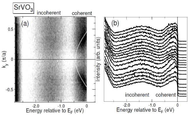
Figure 4: ARPES spectra of SrVO₃ along momentum cut 2 in the Brillouin zone shown in Fig. 5. (a) Intensity plot in the $E$-$k_{y}$ plane. Dispersive feature within $\sim$0.7 eV of $E_{F}$ is the coherent part, while a broad feature around -1.5 eV is the incoherent part. (b) Energy distribution curves (EDC’s).

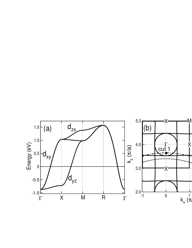
Figure 5: Band structure and the Fermi surface of SrVO₃. (a) Band dispersions obtained by local-density approximation (LDA) band-structure calculation Takegahara . (b)$k_{y}$=0 cross-sectional view of the Fermi surfaces and the momentum loci corresponding to the mapping in Fig. 6.

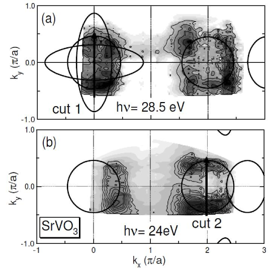
Figure 6: Spectral weight mapping at $E_{F}$ for SrVO₃. (a) Mapping with $h\nu$=28.5eV. (b) Mapping with $h\nu$= 24 eV. Note that the mapping is projection on the $k_{x}$-$k_{y}$ plane.

The band dispersions obtained by local-density approximation (LDA) band-calculation Takegahara are shown in Fig. 5 (a). The hopping parameters of the TB model (1) have been obtained by fitting the TB bands to the results of LDA band-structure calculation Takegahara . Figure 5 (b) illustrates the $k_{y}$=0 cross-sectional view of the Fermi surfaces expressed by the TB model. The three bands correspond to the $d_{xy}$, $d_{yz}$ and $d_{zx}$ orbitals of V and scarcely hybridize with each other. Therefore, these dispersions are almost two-dimensional and form three cylindrical Fermi surfaces intersecting each other around the $\Gamma$ point, although the crystal structure is three-dimensional. The loci of electron momenta in the $k_{x}$-$k_{z}$ plane for constant photon energies $h\nu$= 24 eV and 28.5 eV are plotted in Fig. 5(b). Here, the inner potential of 10 eV has been assumed.

Figure 6 (a) and (b) shows spectral weight mapping in the $k_{x}$-$k_{y}$ space at $E_{F}$ on the momentum loci for the photon energies $h\nu$=28.5 and 24 eV, respectively. The spectral weight for both photon energies are largely confined within the cylindrical Fermi surfaces extended in the $k_{z}$ direction. According to Fig.5(b), cut 2 corresponds to momenta near the X point [$\mathbf{k}=(1,0,0)$]. Therefore, the observed spectral weight comes only from one cylindrical Fermi surface referred to as the $\gamma$ sheet inoueDHVA , which arises from the $d_{xy}$ orbital. On the other hand, the spectral weight in the first BZ for $h\nu$ =28.5 eV (cut 1) is enclosed by the three cylindrical Fermi surfaces inoueDHVA . Indeed, EDC’s along cut 1 [Fig. 7 (c)] show complicated features suggestive of two energy dispersions.

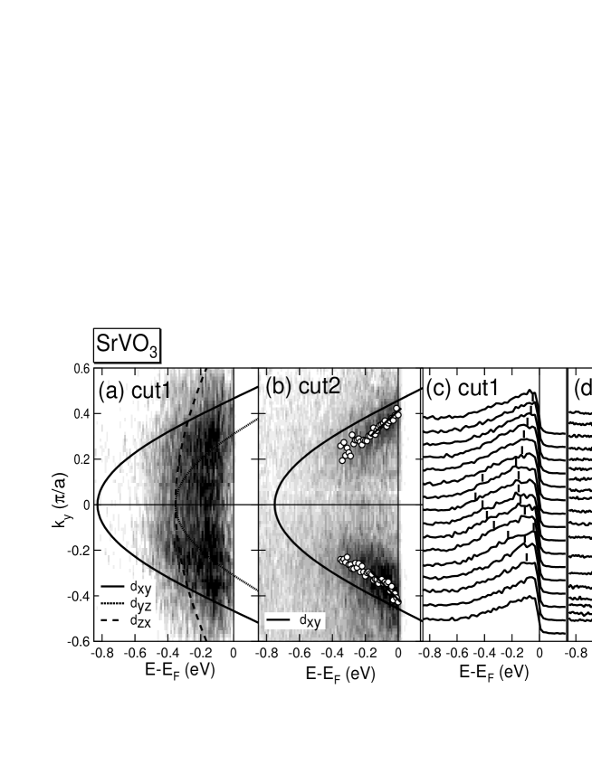
Figure 7: ARPES spectra of SrVO₃ for cuts 1 and 2 in Fig. 5. Panels (a) and (b) show intensity plots in $E$-$k$ space for cuts 1 and cut 2, respectively. Angle-independent backgrounds have been subtracted. Calculated TB band are also superimposed. Circles in (b) are peak positions of MDC’s and represents band dispersion. Panels (c) and (d) are EDC’s corresponding to panels (a) and (b), respectively. Vertical bars are guides to the eye indicating the positions of the dispersive features.

Figure 7(a) and (b) show intensity plots in the energy-momentum ($E$-$k$) space corresponding to each cut in Fig. 5. The $E$-$k_{y}$ plots are compared with the energy dispersions expected from the LDA calculation Takegahara . Figure 7(c) and (d) show EDC’s corresponding to panels (a) and (b), respectively. The EDC’s of cut 1 in panel (c) show parabolic energy dispersions with the bottom at $\sim$-0.5 eV, shallower than that expected from the LDA calculation $\sim$ -0.9 eV. Since the momenta of cut 1 are within the $\alpha$ and $\beta$ sheets of the Fermi surface, there are two dispersions. These dispersions may correspond to the dispersions of the $d_{xy}$ and $d_{yz}$ bands. The dispersion of $d_{zx}$ is not clearly observed in the present plot, probably due to the effect of transition matrix-elements.

For cut 2 [Fig. 7 (b) and (d)], since it does not intersect the $d_{yz}$ and $d_{zx}$ bands, only the $d_{xy}$ band are observed. In panel (b), we have derived the band dispersion for cut 2 from MDC peak positions indicated by circles. By comparing the Fermi velocity of the LDA band structure and that of the present experiment, one can see an overall band narrowing in the measured band dispersion. Near $E_{F}$, we obtain the mass enhancement factor of $m^{*}/m_{b}\sim 1.8\pm 0.2$, which is close to the value $m^{*}/m_{b}=1.98$ obtained from the specific heat coefficient $\gamma$ Inoue2 . Since the LDA calculation predicted that the $d_{xy}$ band is highly two-dimensional and nearly isotropic within the $k_{x}$-$k_{y}$ plane, a similar mass enhancement is expected on the entire Fermi surface.

It has been pointed out that the photoemission spectra of SVO taken at low photon energies have a significant amount of contributions from surface states, particularly in the incoherent part Sekiyama ; Maiti . In order to distinguish bulk from surface contributions in the present spectra, we consider the character of surface states created by the discontinuity of the potential at the surfaces. According to a tight-binding Green’s function formalism for a semi-infinite system Kalstein ; Liebsch , surface-projected density of states of surface-parallel $d_{xy}$ band and surface-perpendicular $d_{yz,zx}$ band have different nature. The surface $d_{xy}$ band does not show an appreciable change from the bulk band because it has the two-dimensional character within the $x$-$y$ plane. In contrast, spectral weight of the surface $d_{yz,zx}$ states is redistributed between the bulk $d_{yz,zx}$ band and the Fermi level SVOARPES , because $k_{z}$ is no longer a good quantum number. This leads to the absence of clear dispersions of the surface $d_{yz,zx}$ bands in ARPES as demonstrated in Ref. SVOARPES . Accordingly, the observed dispersion of the $d_{xy}$ band should represent that of the bulk $d_{xy}$ band.

III.2 La_1-xSr_xFeO₃

LSFO undergoes a pronounced charge disproportionation and an associated MIT around $x\sim 2/3$ Takano . One striking feature of LSFO is that the insulating phase is unusually wide in the phase diagram ($0<x<0.5$ at room temperature and even $0<x<0.7$ at low temperatures) Matsuno . In a previous photoemission study, the gap at the Fermi level ($E_{F}$) was observed for all compositions for $0\leq x\leq 0.67$ Wadati , consistent with the wide insulating region of this system.

ARPES measurements on LSFO were carried out using a photoemission spectroscopy (PES) system combined with a laser molecular beam epitaxy (MBE) chamber, which was installed at beamline BL-1C of Photon Factory, KEK Horiba . The preparation and characterization of the LSFO films are described in Ref. Wadati . By low energy electron diffraction (LEED), sharp $1\times 1$ spots were observed with no sign of surface reconstruction, confirming the well-ordered surfaces of the films. Details of the experimental conditions are described in Ref. LSFOARPES .

The left panel of Fig. 8 (a) shows a gray-scale plot of the experimental band structure obtained by ARPES measurements of an LSFO ($x=0.4$) thin film with the photon energy of 74 eV LSFOARPES . Here, the second derivatives of the EDC’s are plotted on the gray scale, where dark parts correspond to energy bands. In Fig. 8 (b), hole pockets obtained by a TB calculation (described below) are also shown. The trace obtained for $h\nu=74$ eV crosses the calculated hole pocket. The structure at $-1.3$ eV shows a significant dispersion, and is assigned to the Fe $3d$ majority-spin $e_{g}$ bands. The structure at $-2.4$ eV shows a weaker dispersion than the $e_{g}$ bands, and is assigned to the Fe $3d$ $t_{2g}$ majority-spin bands. The structures at $-(4-7)$ eV are assigned to the O $2p$ bands. The $e_{g}$ bands do not cross $E_{F}$, consistent with the insulating behavior and the persistence of the gap observed in the angle-integrated PES (AIPES) spectra Wadati .

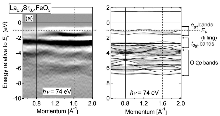
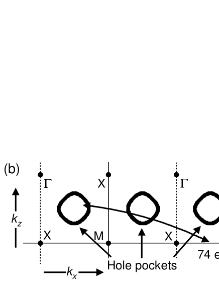
Figure 8: Comparison of ARPES spectra of an LSFO thin film taken at $h\nu=74$ eV with TB calculation. The left panel of (a) shows the experimental band structure (dark parts correspond to energy bands) and the right panel of (a) shows the result of TB calculation. The traces in $k$-space and calculated hole pockets are shown in (b).

The best fit of TB calculation [right panel of Fig. 8 (a)] to the observed band dispersions and the optical gap of 2.1 eV of LaFeO₃ (LFO) opt1 has been obtained with $\epsilon_{d}-\epsilon_{p}$ = 2.65 eV, $(pd\sigma)=-1.5$ eV, and $\Delta E=5.3$ eV. We also considered the effect of $k_{z}$ broadening given by a Lorentzian function as described in Sec. 2.2. Here we have used the value $\lambda=5\ \mbox{\AA}$. $\Delta k_{z}\sim 1/\lambda$ $(\sim 0.2\ \mbox{\AA}^{-1})$ is approximately 10 % of the Brillouin zone ($2\pi/a$). Here, it should be noted that $\epsilon_{d}-\epsilon_{p}$, $(pd\sigma)$ and $\Delta E$ primarily determine the Fe $3d$ $-$ O $2p$ band positions, their dispersions, and the optical band gap, respectively. The dispersions of the $e_{g}$ bands were successfully reproduced. The very weak dispersions of the $t_{2g}$ bands and the width of the O $2p$ bands were also well reproduced by this calculation. The energy position of the calculated $E_{F}$ determined from the filling of electrons was not in agreement with the experimental $E_{F}$, however. This discrepancy corresponds to the fact that this material is insulating up to 70 % hole doping while the rigid-band model based on the band-structure calculation gives the metallic state.

III.3 La_1-xSr_xMnO₃

LSMO has been attracting great interest because of its intriguing properties, such as the CMR effect urushibara and half metallic nature parknat . One end member of LSMO, LaMnO₃, is an antiferromagnetic insulator, and hole-doping induced by the substitution of Sr for La produces a ferromagnetic metallic phase ($0.17<x<0.5$) urushibara .

ARPES measurements on LSMO were carried out using the same system as in the case of LSFO. The preparation and characterization of the LSMO films are described in Refs. horibaLSMO . The surface structure and cleanliness of the films were checked by LEED. Some surface reconstruction-derived spots were observed in addition to sharp $1\times 1$ spots, confirming the well-ordered surfaces of the films, but surface reconstruction is expected to affect the obtained band dispersions. Details of the experimental conditions are described in Ref. Chika .

The left panel of Fig. 9 (a) shows a gray-scale plot of the experimental band structure obtained by ARPES measurements of an LSMO ($x=0.4$) thin film with the photon energy of 88 eV Chika . Here, the second derivatives of the EDC’s are plotted on the gray scale, where dark parts correspond to energy bands as in the case of LSFO along the trace in $k$-space shown in Fig. 9 (b). Note that this trace is approximately along the $\Gamma$-X direction. We shall assume that the trace is exactly along the $\Gamma$-X direction for the moment. The effect of the deviation from the $\Gamma$-X line will be discussed below. Here, electron pockets obtained by a TB calculation are also shown in Fig. 9 (b). One of the Mn $3d$ majority-spin $e_{g}$ bands at $-(0-1)$ eV shows a significant dispersion and crosses $E_{F}$, corresponding to the half metallic behavior parknat . The $E_{F}$ crossing of the $e_{g}$ bands is consistent with the observed Fermi edge in the AIPES spectra horibaLSMO . The Mn $3d$ majority-spin $t_{2g}$ bands at $-(1-2)$ eV show weaker dispersions than the $e_{g}$ bands. The bands at $-(2-3)$ eV shows dispersions with a shorter period in $k$-space than the Brillouin zone. This means that these bands are affected by the surface reconstruction detected in the LEED pattern. The O $2p$ bands are located at $-(4-7)$ eV.

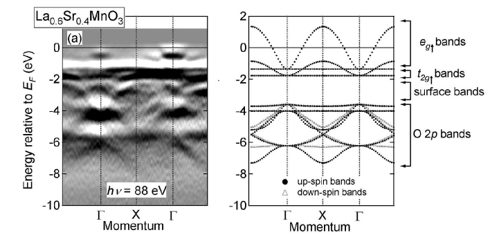
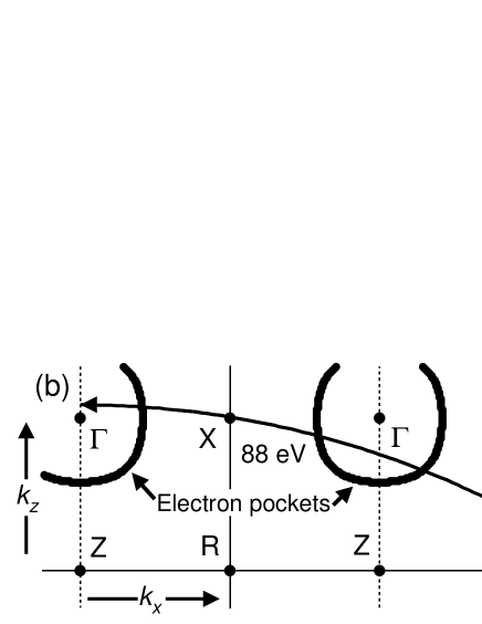
Figure 9: Comparison of ARPES spectra of an LSMO thin film taken at $h\nu=88$ eV and TB calculation. The left panel of (a) shows the experimental band structure (dark parts correspond to energy bands) Chika and the right panel of (a) shows the result of TB calculation. The traces in $k$-space and calculated electron pockets are shown in (b).

The best fit of the TB calculation to the observed band dispersions [right panel of Fig. 9 (a)] has been obtained with $\epsilon_{d}-\epsilon_{p}=5.3$ eV, $(pd\sigma)=-2.0$ eV, and $\Delta E=4.6$ eV. The strong dispersions of the $e_{g}$ bands, the weak dispersions of the $t_{2g}$ bands, and the width of the O $2p$ bands were successfully reproduced, although there are no bands in the calculation corresponding to the experimental surface bands. The bottom of the $e_{g}$ bands is at $\sim-0.5$ eV in the experiment and at $\sim-1.5$ eV in the calculation. This difference may come from the mass renormalization caused by strong electron correlation in this system. One can estimate the mass enhencement to be $m^{\ast}/m_{b}\sim 2.5$.

Figure 10 (a) shows the calculated density of states (DOS) of the FM state. The partial DOS’s for the majority-spin Mn $e_{g}$, the majority-spin Mn $t_{2g}$, the minority-spin Mn $e_{g}$, and the minority-spin Mn $t_{2g}$ orbitals are shown in the lower panels. No band gap opens between the majority-spin $e_{g}$ bands and the minority-spin $t_{2g}$ bands for the present $\Delta E$ value. In Fig. 10 (a), the $E_{F}$ position has been determined from the filling of electrons, and also calculated DOS at $E_{F}$ [$D^{b}(E_{F})$] has been obtained. Using the relationship

$$\gamma^{b}=\frac{\pi^{2}}{3}{k_{B}}^{2}D^{b}(E_{F}),$$ (9)

we obtain the calculated electronic specific heat coefficient by $\gamma^{b}\sim 1$ [mJ mol² K^-2]. The experimental electronic specific heat coefficient has been reported as $\gamma\sim 3.5$ [mJ mol² K^-2] okuda . Thus $m^{\ast}/m_{b}=\gamma/\gamma_{b}\sim 3.5$, in fairly good agreement with $m^{\ast}/m_{b}\sim 2.5$ derived from ARPES, which means that effective mass $m^{\ast}$ is renormalized as

$$m^{\ast}/m_{b}\sim 2.5-3.5.$$ (10)

Figure 10 (b) shows the comparison of the chemical potential shift obtained from the TB calculation in the FM region of LSMO ($0.2\leq x\leq 0.4$ urushibara ; horibaLSMO ) within the rigid-band model (i.e., assuming the constant exchange splitting) and that determined experimentally from core-level photoemission spectra horibaLSMO . The experimental chemical potential shift is slower than the calculated one by a factor of $\sim 0.4$, which means

$$\frac{\partial\mu}{\partial n}\sim\frac{0.4}{D^{b}(E_{F})}.$$ (11)

For a metallic system, the rigid-band picture predicts that

$$\frac{\partial\mu}{\partial n}=\frac{1+F}{D^{\ast}(E_{F})}=\left(\frac{m_{b}}{m^{\ast}}\right)\frac{1+F}{D^{b}(E_{F})},$$ (12)

where $D^{\ast}(E_{F})$ is the DOS of renormalized quasiparticles (QPs) and $F$ is a parameter which represents the effective QP-QP repulsion. From Eqs. (10)-(12), one obtains $F\sim 0-0.4$. This value is much smaller than the values of $F_{0}^{s}$ in AF compounds. For example, it was reported that $F_{0}^{s}\sim 7$ for La_2-xSr_xCuO₄, and $\sim 6$ for La_1-xSr_xVO₃ pote . In the FM case, one obtains small values of $F$ compared to the AF case, probably because of the strong exchange interaction between carriers in the FM case.

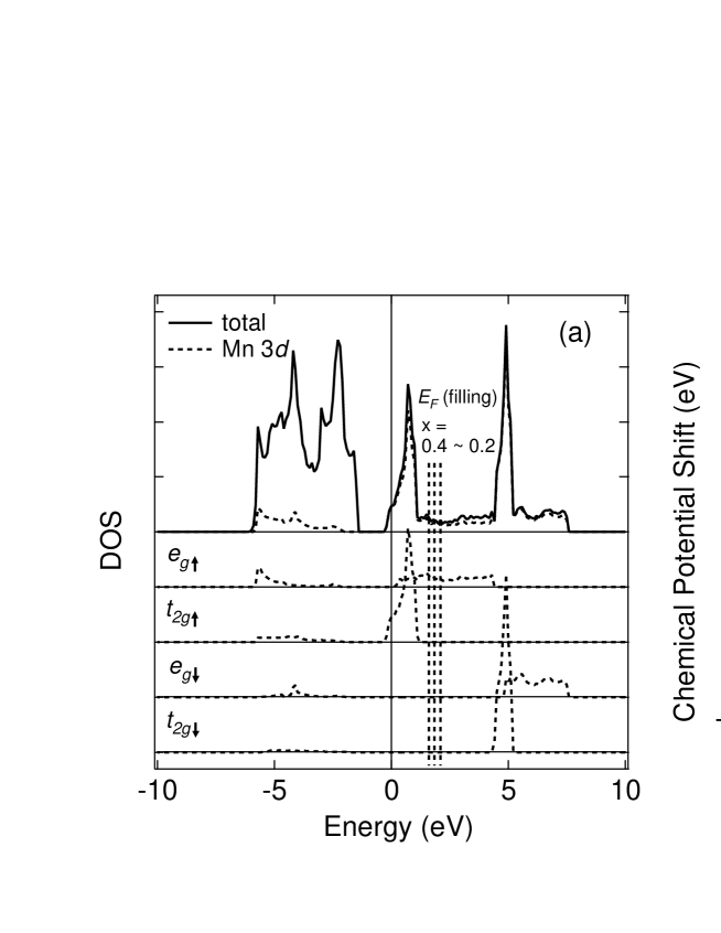
Figure 10: Chemical potential shift in LSMO. (a)DOS obtained from TB calculation. (b)Comparison of the chemical potential shift calculated for the rigid-band-model using TB calculation and that determined experimentally from core-level photoemission spectra horibaLSMO .

Now we go back to the effect of the deviation of the trace with $h\nu=88$ eV from the $\Gamma$-X direction. Figure 11 shows a TB simulation of the ARPES spectra of LSMO taken at 88 eV using the above-mentioned parameter values. Panels (a), (b) and (c) show the results for $\Delta k_{z}=0$ (without $k_{z}$ broadening), $\Delta k_{z}=1/\lambda$, and $\Delta k_{z}=\infty$ (uniform integration in $k_{z}$), respectively. In panel (a), the energy position of the bottom of the $e_{g}$ bands at $k_{\parallel}=0\ \mbox{\AA}^{-1}$ is different from that at $k_{\parallel}=1.6\ \mbox{\AA}^{-1}$, while in panel (b) the bottoms are at almost the same energy positions. In experiment [Fig. 9 (a)], the bottoms are almost at the same energy positions, which means that the experimental results are in good agreement with (b), that is $\Delta k_{z}=1/\lambda$. In panel (c), there are two bands approaching $E_{F}$, in disagreement with experiment.

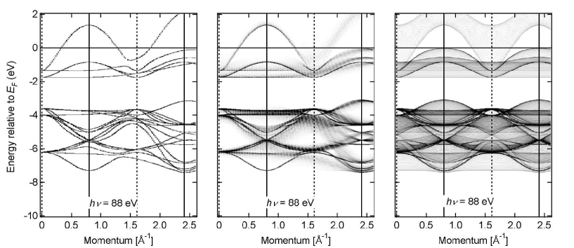
Figure 11: Simulated ARPES spectra of LSMO ($x=0.4$) taken at 88 eV on TB calculation. (a) $\Delta k_{z}=0$, (b) $\Delta k_{z}=1/\lambda$, (c) $\Delta k_{z}=\infty$.

Figure 12 shows comparison of the dispersion along the $\Gamma$-X direction (dots) and simulated spectra (gray scale) obtained assuming $\Delta k_{z}=1/\lambda$ for $h\nu=88$ eV. There are some discrepancies in the high-binding-energy region $-(4-7)$ eV, but the overall agreement is rather good in the region near $E_{F}$ [$-(0-2)$ eV]. This means that one can trace the band dispersions almost along the $\Gamma$-X direction by performing ARPES with a fixed photon energy of $h\nu=88$ eV because of the large $k_{z}$-integrated DOS at a high-symmetry line (in this case the $\Gamma$-X direction). Even if the trace somewhat deviates from a high-symmetry line, one can trace the dispersion along the high-symmetry line due to the large DOS and the effect of $k_{z}$ broadening. By changing the photon energy with changing the emission angle in ARPES measurements, one can map band dispersions precisely along the $\Gamma$-X line. However, the photoionization cross section varies with a photon energy, making the interpretation difficult. In practice, fixing a photon energy and changing an emission angle is a more efficient and useful way to obtain band dispersions in such materials. We also revealed that considering the effect of $k_{z}$ broadening is important for the interpretation of the ARPES of the three-dimensional materials.

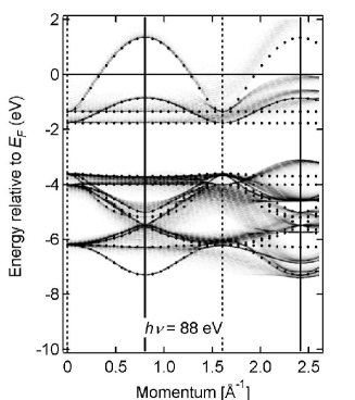
Figure 12: Comparison of the dispersion along the $\Gamma$-X direction (dots) and simulated spectra (gray scale) for LSMO ($x=0.4$) calculated assuming $\Delta k_{z}=1/\lambda$ at 88 eV.

IV Conclusion

We have analyzed the ARPES data of SVO bulk crystals and LSFO ($x=0.4$) and LSMO ($x=0.4$) thin films using TB band-structure calculations. As for SVO, the enhanced effective electron mass obtained from the energy band near $E_{F}$ was consistent with the bulk thermodynamic properties. The experimental band structures of LSFO and LSMO were interpreted using a TB band-structure calculation. The overall agreement between experiment and calculation is fairly good. However, in the case of LSFO, the energy position of the calculated $E_{F}$ was not in agreement with the experimental $E_{F}$, reflecting the insulating behavior. In the case of LSMO, experimental energy bands were narrowed compared with calculation due to strong electron correlation. We also demonstrated that considering the effect of $k_{z}$ broadening is important for the interpretation of the ARPES results of such three-dimensional materials.

Appendix A Basis functions and matrix elements for TB band-structure calculations

Table 1: TB basis functions used in the band-structure calculation of LSFO

	No.	Origin	Function	No.	Origin	Function
Fe $3d$	1	$(0,0,0)$	$xy$	15	$a(1,0,0)$	$xy$
	2	$(0,0,0)$	$yz$	16	$a(1,0,0)$	$yz$
	3	$(0,0,0)$	$zx$	17	$a(1,0,0)$	$zx$
	4	$(0,0,0)$	$3z^{2}-r^{2}$	18	$a(1,0,0)$	$3z^{2}-r^{2}$
	5	$(0,0,0)$	$x^{2}-y^{2}$	19	$a(1,0,0)$	$x^{2}-y^{2}$
O $2p$	6	$\frac{1}{2}a(1,0,0)$	$x$	20	$\frac{1}{2}a(3,0,0)$	$x$
	7	$\frac{1}{2}a(1,0,0)$	$y$	21	$\frac{1}{2}a(3,0,0)$	$y$
	8	$\frac{1}{2}a(1,0,0)$	$z$	22	$\frac{1}{2}a(3,0,0)$	$z$
	9	$\frac{1}{2}a(0,1,0)$	$x$	23	$\frac{1}{2}a(2,1,0)$	$x$
	10	$\frac{1}{2}a(0,1,0)$	$y$	24	$\frac{1}{2}a(2,1,0)$	$y$
	11	$\frac{1}{2}a(0,1,0)$	$z$	25	$\frac{1}{2}a(2,1,0)$	$z$
	12	$\frac{1}{2}a(0,0,1)$	$x$	26	$\frac{1}{2}a(2,0,1)$	$x$
	13	$\frac{1}{2}a(0,0,1)$	$y$	27	$\frac{1}{2}a(2,0,1)$	$y$
	14	$\frac{1}{2}a(0,0,1)$	$z$	28	$\frac{1}{2}a(2,0,1)$	$z$

Table 2: Nonzero matrix elements of the TB Hamiltonian used in the calculation of LSFO. $\xi\equiv k_{x}a$, $\eta\equiv k_{y}a$, and $\zeta\equiv k_{z}a$.

A. $d$-$d$ interactions

$H_{1,1}=H_{2,2}=H_{3,3}=\epsilon_{d}-4Dq-\Delta E/2$, $H_{4,4}=H_{5,5}=\epsilon_{d}+6Dq-\Delta E/2$

$H_{15,15}=H_{16,16}=H_{17,17}=\epsilon_{d}-4Dq+\Delta E/2$, $H_{18,18}=H_{19,19}=\epsilon_{d}+6Dq+\Delta E/2$

B. $p$-$p$ interactions

$C_{1}=\frac{1}{2}(pp\sigma)+\frac{1}{2}(pp\pi)$, $C_{2}=\frac{1}{2}(pp\sigma)-\frac{1}{2}(pp\pi)$, $C_{3}=(pp\pi)$

$H_{6,6}=H_{10,10}=H_{14,14}=H_{20,20}=H_{24,24}=H_{28,28}=\epsilon_{p}$

$H_{7,7}=H_{8,8}=H_{9,9}=H_{11,11}=H_{12,12}=H_{13,13}=\epsilon_{p}$

$H_{21,21}=H_{22,22}=H_{23,23}=H_{25,25}=H_{26,26}=H_{27,27}=\epsilon_{p}$

$H_{6,9}=H_{7,10}=H_{20,23}=H_{21,24}=2C_{1}\cos\left(\frac{1}{2}\xi-\frac{1}{2}\eta\right)$

$H_{6,10}=H_{7,9}=H_{20,24}=H_{21,23}=-2C_{2}\cos\left(\frac{1}{2}\xi-\frac{1}{2}\eta\right)$

$H_{6,12}=H_{8,14}=H_{20,26}=H_{22,28}=2C_{1}\cos\left(\frac{1}{2}\xi-\frac{1}{2}\zeta\right)$

$H_{6,14}=H_{8,12}=H_{20,28}=H_{22,26}=-2C_{2}\cos\left(\frac{1}{2}\xi-\frac{1}{2}\zeta\right)$

$H_{6,23}=H_{7,24}=H_{20,9}=H_{21,10}=2C_{1}\cos\left(\frac{1}{2}\xi+\frac{1}{2}\eta\right)$

$H_{6,24}=H_{7,23}=H_{20,10}=H_{21,9}=2C_{2}\cos\left(\frac{1}{2}\xi+\frac{1}{2}\eta\right)$

$H_{6,26}=H_{8,28}=H_{20,12}=H_{22,14}=2C_{1}\cos\left(\frac{1}{2}\xi+\frac{1}{2}\zeta\right)$

$H_{6,28}=H_{8,26}=H_{20,14}=H_{22,12}=2C_{2}\cos\left(\frac{1}{2}\xi+\frac{1}{2}\zeta\right)$

$H_{7,13}=H_{21,27}=2C_{3}\cos\left(\frac{1}{2}\xi-\frac{1}{2}\zeta\right)$

$H_{7,27}=H_{21,13}=2C_{3}\cos\left(\frac{1}{2}\xi+\frac{1}{2}\zeta\right)$

$H_{8,11}=H_{22,25}=2C_{3}\cos\left(\frac{1}{2}\xi-\frac{1}{2}\eta\right)$

$H_{8,25}=H_{22,11}=2C_{3}\cos\left(\frac{1}{2}\xi+\frac{1}{2}\eta\right)$

$H_{9,12}=H_{23,26}=2C_{3}\cos\left(\frac{1}{2}\eta-\frac{1}{2}\zeta\right)$

$H_{9,26}=H_{23,12}=2C_{3}\cos\left(\frac{1}{2}\eta+\frac{1}{2}\zeta\right)$

$H_{10,13}=H_{11,14}=H_{24,27}=H_{25,28}=2C_{1}\cos\left(\frac{1}{2}\eta-\frac{1}{2}\zeta\right)$

$H_{10,14}=H_{11,13}=H_{24,28}=H_{25,27}=-2C_{2}\cos\left(\frac{1}{2}\eta-\frac{1}{2}\zeta\right)$

$H_{10,27}=H_{11,28}=H_{24,13}=H_{25,14}=2C_{1}\cos\left(\frac{1}{2}\eta+\frac{1}{2}\zeta\right)$

$H_{10,28}=H_{11,27}=H_{24,14}=H_{25,13}=2C_{2}\cos\left(\frac{1}{2}\eta+\frac{1}{2}\zeta\right)$

C. $p$-$d$ interactions

$H_{1,7}=H_{3,8}=H_{15,21}=H_{17,22}=-(pd\pi)\exp\left(i\frac{1}{2}\xi\right)$

$H_{1,9}=H_{2,11}=H_{15,23}=H_{16,25}=-(pd\pi)\exp\left(i\frac{1}{2}\eta\right)$

$H_{1,21}=H_{3,22}=H_{15,7}=H_{17,8}=(pd\pi)\exp\left(-i\frac{1}{2}\xi\right)$

$H_{1,23}=H_{2,25}=H_{15,9}=H_{16,11}=(pd\pi)\exp\left(-i\frac{1}{2}\eta\right)$

$H_{2,13}=H_{3,12}=H_{16,27}=H_{17,26}=-(pd\pi)\exp\left(i\frac{1}{2}\zeta\right)$

$H_{2,27}=H_{3,26}=H_{16,13}=H_{17,12}=(pd\pi)\exp\left(-i\frac{1}{2}\zeta\right)$

$H_{4,6}=H_{18,20}=\frac{1}{2}(pd\sigma)\exp\left(i\frac{1}{2}\xi\right)$

$H_{4,10}=H_{18,24}=\frac{1}{2}(pd\sigma)\exp\left(i\frac{1}{2}\eta\right)$

$H_{4,14}=H_{18,28}=-(pd\sigma)\exp\left(i\frac{1}{2}\zeta\right)$

$H_{4,20}=H_{18,6}=-\frac{1}{2}(pd\sigma)\exp\left(-i\frac{1}{2}\xi\right)$

$H_{4,24}=H_{18,10}=-\frac{1}{2}(pd\sigma)\exp\left(-i\frac{1}{2}\eta\right)$

$H_{4,28}=H_{18,14}=(pd\sigma)\exp\left(-i\frac{1}{2}\zeta\right)$

$H_{5,6}=H_{19,20}=-\frac{\sqrt{3}}{2}(pd\sigma)\exp\left(i\frac{1}{2}\xi\right)$

$H_{5,10}=H_{19,24}=\frac{\sqrt{3}}{2}(pd\sigma)\exp\left(i\frac{1}{2}\eta\right)$

$H_{5,20}=H_{19,6}=\frac{\sqrt{3}}{2}(pd\sigma)\exp\left(-i\frac{1}{2}\xi\right)$

$H_{5,24}=H_{19,10}=-\frac{\sqrt{3}}{2}(pd\sigma)\exp\left(-i\frac{1}{2}\eta\right)$

Table 3: TB basis functions used in the band-structure calculation of LSMO

	No.	Origin	Function		No.	Origin	Function
Fe $3d$	1	$(0,0,0)$	$xy$	O $2p$	6	$\frac{1}{2}a(1,0,0)$	$x$
	2	$(0,0,0)$	$yz$		7	$\frac{1}{2}a(1,0,0)$	$y$
	3	$(0,0,0)$	$zx$		8	$\frac{1}{2}a(1,0,0)$	$z$
	4	$(0,0,0)$	$3z^{2}-r^{2}$		9	$\frac{1}{2}a(0,1,0)$	$x$
	5	$(0,0,0)$	$x^{2}-y^{2}$		10	$\frac{1}{2}a(0,1,0)$	$y$
					11	$\frac{1}{2}a(0,1,0)$	$z$
					12	$\frac{1}{2}a(0,0,1)$	$x$
					13	$\frac{1}{2}a(0,0,1)$	$y$
					14	$\frac{1}{2}a(0,0,1)$	$z$

Table 4: Nonzero matrix elements of the TB Hamiltonian used in the calculation of LSMO. $\xi\equiv k_{x}a$, $\eta\equiv k_{y}a$, and $\zeta\equiv k_{z}a$.

A. $d$-$d$ interactions

$H_{1,1}=H_{2,2}=H_{3,3}=\epsilon_{d}-4Dq-\Delta E/2$ (up spin), $\epsilon_{d}-4Dq+\Delta E/2$ (down spin)

$H_{4,4}=H_{5,5}=\epsilon_{d}+6Dq-\Delta E/2$ (up spin), $\epsilon_{d}+6Dq+\Delta E/2$ (down spin)

B. $p$-$p$ interactions

$C_{1}=\frac{1}{2}(pp\sigma)+\frac{1}{2}(pp\pi)$, $C_{2}=\frac{1}{2}(pp\sigma)-\frac{1}{2}(pp\pi)$, $C_{3}=(pp\pi)$

$H_{6,6}=H_{10,10}=H_{14,14}=\epsilon_{p}$

$H_{7,7}=H_{8,8}=H_{9,9}=H_{11,11}=H_{12,12}=H_{13,13}=\epsilon_{p}$

$H_{6,9}=H_{7,10}=4C_{1}\cos(\frac{1}{2}\xi)\cos(\frac{1}{2}\eta)$

$H_{6,10}=H_{7,9}=-4C_{2}\sin(\frac{1}{2}\xi)\sin(\frac{1}{2}\eta)$

$H_{6,12}=H_{8,14}=4C_{1}\cos(\frac{1}{2}\xi)\cos(\frac{1}{2}\zeta)$

$H_{6,14}=H_{8,12}=-4C_{2}\sin(\frac{1}{2}\xi)\sin(\frac{1}{2}\zeta)$

$H_{7,13}=4C_{3}\cos(\frac{1}{2}\xi)\cos(\frac{1}{2}\zeta)$, $H_{8,11}=4C_{3}\cos(\frac{1}{2}\xi)\cos(\frac{1}{2}\eta)$

$H_{9,12}=4C_{3}\cos(\frac{1}{2}\eta)\cos(\frac{1}{2}\zeta)$

$H_{10,13}=H_{11,14}=4C_{1}\cos(\frac{1}{2}\eta)\cos(\frac{1}{2}\zeta)$

$H_{10,14}=H_{11,13}-4C_{2}\sin(\frac{1}{2}\eta)\sin(\frac{1}{2}\zeta)$

C. $p$-$d$ interactions

$H_{1,7}=H_{3,8}=-2i(pd\pi)\sin(\frac{1}{2}\xi)$

$H_{1,9}=H_{2,11}=-2i(pd\pi)\sin(\frac{1}{2}\eta)$

$H_{2,13}=H_{3,12}=-2i(pd\pi)\sin(\frac{1}{2}\zeta)$

$H_{4,6}=i(pd\sigma)\sin(\frac{1}{2}\xi)$, $H_{4,10}=i(pd\sigma)\sin(\frac{1}{2}\eta)$

$H_{4,14}=-2i(pd\sigma)\sin(\frac{1}{2}\zeta)$, $H_{5,6}=-\sqrt{3}i(pd\sigma)\sin(\frac{1}{2}\xi)$

$H_{5,10}=\sqrt{3}i(pd\sigma)\sin(\frac{1}{2}\eta)$

References

- (1) M. Imada, A. Fujimori, and Y. Tokura, Rev. Mod. Phys. 70, 1039 (1998).
- (2) J. Zaanen, G. A. Sawatzky, and J. W. Allen, Phys. Rev. Lett. 55, 418 (1985).
- (3) T. Yoshida, K. Tanaka, H. Yagi, A. Ino, H. Eisaki, A. Fujimori, and Z.-X. Shen, Phys. Rev. Lett. 95, 146404 (2005).
- (4) M. Izumi, Y. Konishi, T. Nishihara, S. Hayashi, M. Shinohara, M. Kawasaki, and Y. Tokura, Appl. Phys. Lett. 73, 2497 (1998).
- (5) J. Choi, C. B. Eom, G. Rijnders, H. Rogalla, and D. H. A. Blank, Appl. Phys. Lett. 79, 1447 (2001).
- (6) K. Horiba, H. Oguchi, H. Kumigashira, M. Oshima, K. Ono, N. Nakagawa, M. Lippmaa, M. Kawasaki, and H. Koinuma, Rev. Sci. Instr. 74, 3406 (2003).
- (7) M. Shi, M. C. Falub, P. R. Willmott, J. Krempasky, R. Herger, K. Hricovini, and L. Patthey, Phys. Rev. B 70, 140407 (2004).
- (8) A. Chikamatsu, H. Wadati, H. Kumigashira, M. Oshima, A. Fujimori, N. Hamada, T. Ohnishi, M. Lippmaa, K. Ono, M. Kawasaki, and H. Koinuma, cond-mat/0503373, Phys. Rev. B, in press.
- (9) H. Wadati, A. Chikamatsu, M. Takizawa, R. Hashimoto, H. Kumigashira, T. Yoshida, T. Mizokawa, A. Fujimori, M. Oshima, M. Lippmaa, M. Kawasaki, and H. Koinuma, cond-mat/0603333.
- (10) V. N. Strocov, J. Electron Spectrosc. Relat. Phenom. 130, 65 (2003).
- (11) A. Liebsch, Phys. Rev. Lett. 90, 096401 (2003).
- (12) A. H. Kahn and A. J. Leyendecker, Phys. Rev. 135, A1321 (1964).
- (13) L. F. Mattheiss, Phys. Rev. 181, 987 (1969).
- (14) L. F. Mattheiss, Phys. Rev. B 6, 4718 (1972).
- (15) J. C. Slater and G. F. Koster, Phys. Rev. 94, 1498 (1954).
- (16) W. A. Harrison, Electronic Structure and the Properties of Solids (Dover, New York, 1989).
- (17) L. F. Mattheiss, Phys. Rev. B 5, 290 (1972).
- (18) A. E. Bocquet, T. Mizokawa, T. Saitoh, H. Namatame, and A. Fujimori, Phys. Rev. B 46, 3771 (1992).
- (19) H. Wadati, D. Kobayashi, H. Kumigashira, K. Okazaki, T. Mizokawa, A. Fujimori, K. Horiba, M. Oshima, N. Hamada, M. Lippmaa, M. Kawasaki, and H. Koinuma, Phys. Rev. B 71, 035108 (2005).
- (20) I. H. Inoue, I. Hase, Y. Aiura, A. Fujimori, Y. Haruyama, T. Maruyama, and Y. Nishihara, Phys. Rev. Lett. 74, 2539 (1995).
- (21) I. H. Inoue, O. Goto, H. Makino, N. E. Hussey, and M. Ishikawa, Phys. Rev. B 58, 4372 (1998).
- (22) A. Sekiyama, H. Fujiwara, S. Imada, S. Suga, H. Eisaki, S. I. Uchida, K. Takegahara, H. Harima, Y. Saitoh, I. A. Nekrasov, G. Keller, D. E. Kondakov, A. V. Kozhevnikov, T. Pruschke, K. Held, D. Vollhardt, and V. I. Anisimov, Phys. Rev. Lett. 93, 156402 (2004).
- (23) K. Takegahara, J. Electron Spectrosc. Relat. Phenom. 66, 303 (1994).
- (24) I. H. Inoue, C. Bergemann, I. Hase, and S. R. Julian, Phys. Rev. Lett. 88, 236403 (2002).
- (25) K. Maiti, P. Mahadevan, and D. D. Sarma, Phys. Rev. Lett. 80, 2885 (1998).
- (26) D. Kalkstein and P. Soven, Surf. Sci. 26, 85 (1971).
- (27) M. Takano, J. Kawachi, N. Nakanishi, and Y. Takeda, J. Solid. State Chem. 39, 75 (1981).
- (28) J. Matsuno, T. Mizokawa, A. Fujimori, K. Mamiya, Y. Takeda, S. Kawasaki, and M. Takano, Phys. Rev. B 60, 4605 (1999).
- (29) T. Arima, Y. Tokura, and J. B. Torrance, Phys. Rev. B 48, 17006 (1993).
- (30) A. Urushibara, Y. Moritomo, T. Arima, A. Asamitsu, G. Kido, and Y. Tokura, Phys. Rev. B 51, 14103 (1995).
- (31) J.-H. Park, E. Vescovo, H.-J. Kim, C. Kwon, R. Ramesh, and T. Venkatesan, Nature 392, 794 (1998).
- (32) K. Horiba, A. Chikamatsu, H. Kumigashira, M. Oshima, N. Nakagawa, M. Lippmaa, K. Ono, M. Kawasaki, and H. Koinuma, Phys. Rev. B 71, 155420 (2005).
- (33) T. Okuda, A. Asamitsu, Y. Tomioka, T. Kimura, Y. Taguchi, and Y. Tokura, Phys. Rev. Lett. 81, 3203 (1998).
- (34) A. Fujimori, A. Ino, J. Matsuno, T. Yoshida, K. Tanaka, and T. Mizokawa, J. Electron Spectrosc. Relat. Phenom. 124, 127 (2002).