Abstract

We present an analysis leading to a conjecture on the exact location of the multicritical point in the phase diagram of spin glasses in finite dimensions. The conjecture, in satisfactory agreement with a number of numerical results, was previously derived using an ansatz emerging from duality and the replica method. In the present paper we carefully examine the ansatz and reduce it to a hypothesis on analyticity of a function appearing in the duality relation. Thus the problem is now clearer than before from a mathematical point of view: The ansatz, somewhat arbitrarily introduced previously, has now been shown to be closely related to the analyticity of a well-defined function.

1 Introduction

To establish reliable analytical theories of spin glasses has been one of the most challenging problems in statistical physics for years. The problem was solved for the mean-field model [1, 2, 3, 4]. Much less is known analytically for finite-dimensional spin glasses, for which approximate methods including numerical simulations and phenomenological theories [5] have been the main tools of investigation in addition to a limited set of rigorous results and exact solutions [6, 7].

Our main interest in the present contribution does not lie directly in the issue of the properties of the spin glass phase. We instead will concentrate ourselves on the precise (and possibly exact) determination of the structure of phase diagram of finite-dimensional spin glasses. This problem is of practical importance for numerical studies since exact values of transition points greatly facilitate reliable estimates of critical exponents in finite-size scaling.

More precisely, recent developments [8, 9, 10, 11, 12] to derive a conjecture on the exact location of the multicritical point in the phase diagram will be analyzed from a different view point. The conjecture was derived using the replica method, gauge symmetry and a duality relation. In addition it was necessary to introduce an ansatz to identify the location of a singularity of the free energy. The resulting conjecture for the transition point (multicritical point) is nevertheless in satisfactory agreement with a number of numerical results, which renders a strong support to the validity of our prescription. In the present paper we present a more systematic analysis leading to the ansatz, thus reducing the problem to that of the analyticity proof of a function related to duality. The ansatz was introduced somewhat arbitrarily previously. The discussions in the present paper make it clear that the ansatz is closely related to the analyticity of a well-defined function, which paves a path toward the formal proof of the conjecture.

2 Duality relation for the replicated system

For simplicity, let us consider the $\pm J$ Ising model on the square lattice. It is possible to apply the same line of argument as presented below to other systems (non-Ising models and/or other lattices) as will be mentioned in the final section. The Hamiltonian is

$$H=-J\sum_{\langle ij\rangle}\tau_{ij}S_{i}S_{j},$$ (1)

where $\tau_{ij}=\pm 1$ is a quenched random variable with asymmetric distribution and $J>0$. Periodic boundary conditions are imposed. We accept the replica method in this paper and do not strive to rigorously justify the validity of taking the limit $n\to 0$ in the end, where $n$ is the number of replicas.

The $n$-replicated partition function after configurational average is a function of edge Boltzmann factors:

$$[Z^{n}]\equiv Z_{n}(x_{0}(K,K_{p}),x_{1}(K,K_{p}),\cdots,x_{n}(K,K_{p})).$$ (2)

Here the square brackets denote the configurational average, $K$ stands for $\beta J=J/k_{B}T$, and $K_{p}$ is a function of $p$ (the probability that $\tau_{ij}$ is 1) defined through $e^{-2K_{p}}=(1-p)/p$. The $k$th edge Boltzmann factor $x_{k}(K,K_{p})~{}(k=0,1,\cdots,n)$ represents the configuration-averaged Boltzmann factor for interacting spins with $k$ antiparallel spin pairs among $n$ nearest-neighbor pairs for a bond (edge) as illustrated in Fig. 1,

$$x_{k}(K,K_{p})=pe^{(n-2k)K}+(1-p)e^{-(n-2k)K}.$$ (3)

Figure 1: The edge Boltzmann factor $x_{k}(K,K_{p})$ represents the weight for $k$ antiparallel spin pairs among $n$ nearest-neighboring pairs. The case of $k=1,n=4$ is shown here.

The expression on the right-hand side of Eq. (2) emphasizes the fact that the system properties are uniquely determined by the values of edge Boltzmann factors because the interactions (or equivalently, the edge Boltzmann factors) do not depend on the bond index $\langle ij\rangle$ after the configurational average.

The formulation of duality transformation developed by Wu and Wang [13] can be applied to the function $Z_{n}$ of Eq. (2) to derive a dual partition function on the dual square lattice with dual edge Boltzmann factors. The result is, up to a trivial constant, [9]

$$Z_{n}(x_{0},x_{1},\cdots,x_{n})=Z_{n}(x_{0}^{*},x_{1}^{*},\cdots,x_{n}^{*}).$$ (4)

The dual Boltzmann factors are discrete multiple Fourier transforms of the original Boltzmann factors (which are simple combinations of plus and minus of the original Boltzmann factors in the case of Ising spins):

$$2^{n/2}x_{m}^{*}=\sum_{k=0}^{n}D_{m}^{k}\,x_{k},$$ (5)

where the $D_{m}^{k}$ are the coefficients of the expansion of $(1-t)^{m}(1+t)^{n-m}$ :

$$(1-t)^{m}(1+t)^{n-m}=\sum_{k=0}^{n}D_{m}^{k}\,t^{k},$$ (6)

or explicitly,

$$D_{m}^{k}=\sum_{l=0}^{k}(-1)^{l}{m\choose l}{n-m\choose k-l}.$$ (7)

For example, in the case of $n=2$, the dual Boltzmann factors are given as

$$\begin{array}[]{rcl}2\,x_{0}^{*}&=&(x_{0}+x_{1})+(x_{1}+x_{2})=x_{0}+2x_{1}+x_{2}\\ 2\,x_{1}^{*}&=&(x_{0}-x_{1})+(x_{1}-x_{2})=x_{0}-x_{2}\\ 2\,x_{2}^{*}&=&(x_{0}-x_{1})-(x_{1}-x_{2})=x_{0}-2x_{1}+x_{2}.\end{array}$$ (8)

It will be useful to measure the energy from the all-parallel spin configuration ($k=0$) and, correspondingly, factor out the principal Boltzmann factors, $x_{0}$ (left hand side) and $x_{0}^{*}$ (right hand side), from both sides of Eq. (4). Since the partition function is a homogeneous multinomial of edge Boltzmann factors $(x_{0},x_{1},\cdots,x_{n})$ of order $N_{B}$ (the number of bonds), the duality relation (4) can then be rewritten as

$$(x_{0})^{N_{B}}\tilde{\mathcal{Z}}_{n}(u_{1},u_{2},\cdots,u_{n})=(x_{0}^{*})^{N_{B}}\tilde{\mathcal{Z}}_{n}(u_{1}^{*},u_{2}^{*},\cdots,u_{n}^{*}),$$ (9)

using the normalized edge Boltzmann factors $u_{k}$ and $u_{k}^{*}~{}(k=1,2,\cdots,n)$ defined by $u_{k}=x_{k}/x_{0}$ and $u_{k}^{*}=x_{k}^{*}/x_{0}^{*}$.

The discussions so far have already been given in references [9, 10, 11]. In those papers we went on to try to identify the multicritical point by the fixed-point condition of the principal Boltzmann factor, $x_{0}(K,K_{p})=x_{0}^{*}(K,K_{p})$, combined with the Nishimori line (NL) condition $K=K_{p}$ [6]. The reason for the latter choice is that the multicritical point is expected to lie on the NL [14]. In this way an ansatz was made at this stage that the multicritical point is given by the relation $x_{0}(K,K)=x_{0}^{*}(K,K)$. The resulting expression for the location of the multicritical point was confirmed to be exact in the cases of $n=1,2$ and $n\to\infty$. Extrapolation to the quenched limit $n\to 0$ gave results in agreement with a number of independent numerical estimates as listed in Table 1. However, it was difficult to understand the mathematical origin of the somewhat arbitrary-looking ansatz.

We develop an argument in the next section to justify the above-mentioned relation $x_{0}(K,K)=x_{0}^{*}(K,K)$ as the fixed point condition of duality relation for the replicated $\pm J$ Ising model on the NL.

3 Self-duality

The duality relation (9) applies to an arbitrary set of parameter values $(K,K_{p})$ or an arbitrary point in the phase diagram (Fig. 2).

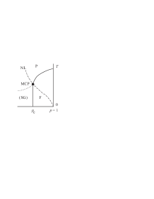
Figure 2: A typical phase diagram of the $\pm J$ Ising model. Shown dash-dotted is the NL. Note that the spin glass phase is believed not to exist in two dimensions. The multicritical point is denoted as MCP.

However, we restrict ourselves to the NL ($K=K_{p}$) to investigate the location of the multicritical point. Then Eq. (9) is expressed as

$$(x_{0}(K))^{N_{B}}\tilde{\mathcal{Z}}_{n}(u_{1}(K),u_{2}(K),\cdots,u_{n}(K))=(x_{0}^{*}(K))^{N_{B}}\tilde{\mathcal{Z}}_{n}(u_{1}^{*}(K),u_{2}^{*}(K),\cdots,u_{n}^{*}(K))$$ (10)

since $x_{0},u_{1},\cdots,u_{n}$ and $x_{0}^{*},u_{1}^{*},\cdots,u_{n}^{*}$ are now functions of a single variable $K$.

It is difficult to apply directly the usual duality argument (identification of a fixed point with the transition point assuming uniqueness of the latter) to Eq. (10). The reason is that $\tilde{\mathcal{Z}}_{n}$ is a multi-variable function: The two trajectories representing $\mathcal{L}(K)\stackrel{{\scriptstyle\rm def}}{{=}}(u_{1}(K),u_{2}(K),\cdots,u_{n}(K))$ and $\mathcal{L}^{*}(K)\stackrel{{\scriptstyle\rm def}}{{=}}(u_{1}^{*}(K),u_{2}^{*}(K),\cdots,u_{n}^{*}(K))$ do not in general coincide as depicted in Fig. 3. In other words, there is no fixed point in the conventional sense for the present system.

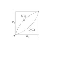
Figure 3: Trajectories of the points $\mathcal{L}(K)=(u_{1}(K),u_{2}(K),\cdots,u_{n}(K))$ and $\mathcal{L}^{*}(K)=(u_{1}^{*}(K),u_{2}^{*}(K),\cdots,u_{n}^{*}(K))$, projected onto the $(u_{1},u_{2})$ plane. The arrows indicate the sense of motion of $\mathcal{L}(K)$ and $\mathcal{L}^{*}(K)$ as $K$ changes from 0 to $\infty$.

In spite of this difficulty of the apparent absence of a fixed point, we now show that it is still possible to devise a map which renders the present replicated system self-dual with a fixed point. To derive such a result, it is useful to note a few properties of the quantities appearing in Eq. (10).

Lemma 1

The normalized Boltzmann factor $u_{k}(K)$ is a monotone decreasing function of $K$ from $u_{k}(0)=1$ to $\lim_{K\to\infty}u_{k}(K)=0$. The dual $u_{k}^{*}(K)$ is a monotone increasing function from $u_{k}^{*}(0)=0$ to $\lim_{K\to\infty}u_{k}^{*}(K)=1$. Here $k\in\{1,2,\cdots n\}$ and $n\in\mathbb{N}$.

Proof. From the definition (3) of $x_{k}$ and the NL condition $K=K_{p}$ (i.e. $e^{-2K}=(1-p)/p)$, it is straightforward to verify that

$$u_{k}(K)=\frac{e^{(n+1-2k)K}+e^{-(n+1-2k)K}}{e^{(n+1)K}+e^{-(n+1)K}},$$ (11)

from which the result for $u_{k}(K)$ follows. The dual are shown to satisfy [9]

$$u_{k}^{*}(K)=\left\{\begin{array}[]{ll}(\tanh K)^{k+1}&(k~{}{\rm odd})\\ (\tanh K)^{k}&(k~{}{\rm even})\end{array}\right.,$$ (12)

which leads to the statement on $u_{k}^{*}$.  

Lemma 2

The normalized partition function $\tilde{\mathcal{Z}}_{n}(u_{1},\cdots,u_{n})$ is a monotone increasing continuous function of all of its arguments $u_{1},\cdots,u_{n}$ with the limiting values in the hypercube $[0,1]^{n}$ $\tilde{\mathcal{Z}}_{n}(0,\cdots,0)=2$ and $\tilde{\mathcal{Z}}_{n}(1,\cdots,1)=2^{nN}$, where $N$ is the number of sites.

Proof. Since the normalized partition function is a multinomial of normalized edge Boltzmann factors $u_{1},\cdots,u_{n}$ with positive coefficients, the first half of the above statement is trivial. To check the second half, we note that $u_{1}=\cdots=u_{n}=0$ corresponds to the case where no antiparallel spin pairs are allowed in any replica at any bond. The only allowed spin configuration is the all-parallel (i.e. perfectly ferromagnetic) one, for which we have set the energy 0 (or the edge Boltzmann factor $u_{0}=1$) since the energy is measured from such a state by dividing $x_{k}$ by $x_{0}$. Taking into account the global inversion degeneracy, we conclude that $\tilde{\mathcal{Z}}_{n}(0,\cdots,0)$ is equal to $2u_{0}=2$.

Similarly, when $u_{1}=\cdots=u_{n}=1$ (corresponding to the high-temperature limit), all spin configurations show up with equal probability. Therefore the normalized partition function just counts the number of possible spin configurations, yielding $2^{nN}$.  

Now we are ready to step toward the main theorems.

Theorem 1

There exists a monotone decreasing function $d(K)$ with $\lim_{K\to 0}d(K)\to\infty$ and $lim_{K\to\infty}d(K)=0$ by which the value of $\tilde{\mathcal{Z}}$ at $(u_{1}^{*}(K),\cdots,u_{n}^{*}(K))$ becomes equal to the value at $(u_{1}(d(K)),\cdots,u_{n}(d(K)))$,

$$\tilde{\mathcal{Z}}_{n}(u_{1}^{*}(K),\cdots,u_{n}^{*}(K))=\tilde{\mathcal{Z}}_{n}(u_{1}(d(K)),\cdots,u_{n}(d(K))).$$ (13)

Proof. According to Lemma 1, the curve $\mathcal{L}(K)=(u_{1}(K),\cdots,u_{n}(K))$ starts from the point $(1,\cdots,1)$ and ends at $(0,\cdots,0)$ as $K$ increases from 0 to $\infty$. Similarly, the curve $\mathcal{L}^{*}(K)=(u_{1}^{*}(K),\cdots,u_{n}^{*}(K))$ starts from $(0,\cdots,0)$ and ends at $(1,\cdots,1)$. Thus $\tilde{\mathcal{Z}}_{n}(u_{1}(K),\cdots,u_{n}(K))\stackrel{{\scriptstyle\rm def}}{{=}}\mathcal{U}(K)$ is continuous and monotone decreasing from $\mathcal{U}(0)=2^{nN}$ to $\lim_{K\to\infty}\mathcal{U}(K)=2$ by Lemma 2. Similarly, $\tilde{\mathcal{Z}}_{n}(u_{1}^{*}(K),\cdots,u_{n}^{*}(K))\stackrel{{\scriptstyle\rm def}}{{=}}\mathcal{V}(K)$ is continuous and monotone increasing from $\mathcal{V}(0)=2$ to $\lim_{K\to\infty}\mathcal{V}(K)=2^{nN}$. Consequently there exists a monotone decreasing function $d(K)$ (satisfying $\lim_{K\to 0}d(K)\to\infty$ and $lim_{K\to\infty}d(K)=0$) that relates the values of $\mathcal{U}$ and $\mathcal{V}$ such that $\mathcal{U}(d(K))=\mathcal{V}(K)$.  

Corollary 1

The normalized partition function satisfies the duality relation

$$(x_{0}(K))^{N_{B}}\tilde{\mathcal{Z}}_{n}(u_{1}(K),\cdots,u_{n}(K))=(x_{0}^{*}(K))^{N_{B}}\tilde{\mathcal{Z}}_{n}(u_{1}(d(K)),\cdots,u_{n}(d(K))),$$ (14)

where $d(K)$ is the monotone decreasing function shown to exist in Theorem 1.

Proof. Immediate from Eq. (10) and Theorem 1.

Theorem 2

The normalized partition function is self-dual with a fixed point $K_{0}$ given by $K_{0}=d(K_{0})$, which is equivalent to $x_{0}(K_{0})=x_{0}^{*}(K_{0})$.

Proof. The first half of the statement is immediate from Corollary 1. The second half comes from the observation that the values of $\tilde{\mathcal{Z}}_{n}$ on both sides of Eq. (14) become identical at the fixed point $K_{0}=d(K_{0})$, thus making the prefactors, $x_{0}(K)$ and $x_{0}^{*}(K)$, equal to each other.

Corollary 2

Assume that $d(K)$ has no singularity for $K\in[0,\infty)$. If the free energy per site of the replicated system has a unique singularity at some $K=K_{c}$ in the thermodynamic limit, then $K_{c}$ is equal to $K_{0}$ of Theorem 2.

Note. As long as $d(K)$ is analytic, the above statement is the same one as the usual duality argument for the ferromagnetic Ising model on the square lattice, in which $d(K)$ is $-(1/2)\log\tanh K$. However, if $d(K)$ happens to be singular at $K_{1}$ for example, this singularity would be reflected in the singularity of the free energy (away from the fixed point $K_{0}$) through the relation (14): The free energy per spin derived from the right-hand side will be singular at $K_{1}$ reflecting the singularity of $d(K)$ there. This causes a singularity of the free energy derived from the left-hand side at $K_{1}$.

We have been unable to prove analyticity of $d(K)$. This is one of the reasons that the following two statements are conjectures. The other reasons include the validity of the replica method and the absence of a formal proof for the existence of the multicritical point on the NL.

Conjecture 1

[9, 8] The exact location of the multicritical point for the $n$-replicated $\pm J$ Ising model on the square lattice is given by the relation $x_{0}=x_{0}^{*}$ with $K=K_{p}$, i.e.

$$e^{(n+1)K_{c}}+e^{-(n+1)K_{c}}=2^{-n/2}(e^{K_{c}}+e^{-K_{c}})^{n}.$$ (15)

Note. The explicit expressions of $x_{0}$ and $x_{0}^{*}$ are given in Eqs. (3) and (5). See also references [9, 10, 11].

Conjecture 2

[9, 8] The exact location of the multicritical point for the $\pm J$ Ising model on the square lattice with quenched randomness is given by the formula

$$-p_{c}\log p_{c}-(1-p_{c})\log(1-p_{c})=\frac{\log 2}{2}.$$ (16)

Proof. The limit $n\to 0$ of Eq. (15) and the NL condition $K=K_{P}$ yields the above formula.

4 Concluding remarks

The main physical conclusions, Conjecture 1 and Conjecture 2, are not new. The significance of the present paper is that we have derived the ansatz to identify the multicritical point, $x_{0}(K)=x_{0}^{*}(K)$, from the assumption of analyticity of the function $d(K)$, thus hopefully coming a little closer to the formal proof of the conjecture.

In this paper we have limited ourselves to the $\pm J$ Ising model on the square lattice for simplicity. It is straightforward to apply the same type of argument to other lattices and other models. For example, models on the square lattice (such as the Gaussian Ising spin glass and the random chiral Potts model) can be treated very similarly: The differences lie only in the explicit expressions of $x_{k}$ as given in section 2.9 of reference [9] and section 4.1 of reference [11]. Also, the duality structure of the four-dimensional random plaquette gauge model is exactly the same as the $\pm J$ Ising model on the square lattice [10], and therefore the present analysis applies without change. In the case of mutually dual pairs of lattices, such as the triangular and hexagonal lattices or the three-dimensional $\pm J$ Ising model and the three-dimensional random-plaquette gauge model, a simple generalization suffices that refers to the composite duality relation of the two systems, $x_{0}(K_{1})x_{0}(K_{2})=x_{0}^{*}(K_{2})x_{0}^{*}(K_{1})$, where $K_{1}$ is the critical point for one of the systems and $K_{2}$ is for its dual, as detailed around Eq. (17) of reference [11].

Let us next give a few remarks on the comparison with numerics in Table 1. As is seen there, our conjecture agrees with a number of numerical results but lies slightly outside error bars for some instances for the square lattice, 0.8907(2) [17] and 0.8906(2) [18] vs. 0.889972 of our conjecture. A similar situation is observed for three pairs of mutually dual hierarchical lattices analyzed in [25]: The sum of the values of binary entropy $H(p)=-p\log_{2}p-(1-p)\log_{2}(1-p)$ for the pair of mutually dual multicritical points is exactly equal to 1 according to our conjecture, whereas the numerical results are not precisely unity, 1.0172, 0.9829 and 0.9911. We have no definite ideas at the present moment where these subtle differences come from. Further investigations are necessary.

The final remark is on the transition points away from the NL (or the shape of the phase boundary away from the multicritical point). We expect (but cannot prove) that the relation $x_{0}(K,K_{p})=x_{0}^{*}(K,K_{p})$ gives the true critical point only on the NL. An important reason is that the limiting behavior of the transition point as $p\to 1$, derived from the ansatz $x_{0}(K,K_{p})=x_{0}^{*}(K,K_{p})$, shows a deviation from a perturbational result, see [8]. The particularly high symmetry of the system on the NL [27] could be a reason for the success only on the NL.

Model	Numerical estimates	Reference	Our conjecture	Reference
SQ Ising	0.8900(5)	[15]	0.889972	[8, 9]
	0.8894(9)	[16]
	0.8907(2)	[17]
	0.8906(2)	[18]
	0.8905(5)	[19]
SQ Gaussian	1.00(2)	[20]	1.021770	[8, 9]
SQ 3-Potts	0.079-0.080	[21]	0.079731	[8, 9]
$4d$ gauge (RPGM)	0.890(2)	[22]	0.889972	[10]
TR	0.8355(5)	[15]	0.835806	[12]
HEX	0.9325(5)	[15]	0.932704	[12]
$3d$ Ising (RBIM)	0.7673(3)$(=p_{c1})$	[23]	—
$3d$ gauge (RPGM)	0.967(4)$(=p_{c2})$	[24]	—
RBIM+RPGM	$H(p_{c1})+H(p_{c2})=0.99(2)$		$H(p_{c1})+H(p_{c2})=1$	[11]
Hierarchical 1 (H1)	0.8265$(=p_{c3})$	[25]	—
Dual of H1 (dH1)	0.93380$(=p_{c4})$	[25]	—
H1+dH1	$H(p_{c3})+H(p_{c4})=1.0172$		$H(p_{c3})+H(p_{c4})=1$	[11]
Hierarchical 2 (H2)	0.8149$(=p_{c5})$	[25]	—
Dual of H2 (dH2)	0.94872$(=p_{c6})$	[25]	—
H2+dH2	$H(p_{c5})+H(p_{c6})=0.9829$		$H(p_{c5})+H(p_{c6})=1$	[11]
Hierarchical 3 (H3)	0.7527$(=p_{c7})$	[25]	—
Dual of H3 (dH3)	0.97204$(=p_{c8})$	[25]	—
H3+dH3	$H(p_{c7})+H(p_{c8})=0.9911$		$H(p_{c7})+H(p_{c8})=1$	[11]
Hierarchical 4	0.8902(4)	[26]	0.889972	[9, 10]

Table 1: Location of the multicritical point by recent numerical studies and our conjecture. SQ stands for the square lattice, and TR/HEX for the triangular/hexagonal lattices, respectively. RBIM stands for the random-bond Ising model and RPGM is for the random-plaquette gauge model. See reference [25] for the explicit definition of three types of hierarchical lattices (H1, H2, H3) and their duals. Hierarchical 4 is a self-dual lattice, for which the analysis in [9, 10] applies directly (though not stated explicitly in these references). The values are for $p_{c}$ of the $\pm J$ model except for the Gaussian randomness on the square lattice for which the values 1.00(2) and 1.021770 are for $J_{0c}/J$. Spin variables are Ising excepting the three-state Potts model as indicated. The symbol $H(p)$ is for the binary entropy $H(p)=-p\log_{2}p-(1-p)\log_{2}(1-p)$.

References

- [1] D. Sherrington and S. Kirkpatrick, Phys. Rev. Lett. 35, 1792 (1975).
- [2] M. Mézard, G. Parisi and M. A. Virasoro, Spin Glass Theory and Beyond (World Scientific, Singapore, 1987).
- [3] F. Guerra, Commun. Math. Phys. 233, 1 (2003).
- [4] M. Talagrand, (this issue).
- [5] A. P. Young (ed), Spin Glasses and Random Fields (World Scientific, Singapore, 1997).
- [6] H. Nishimori, Statistical Physics of Spin Glasses and Information Processing: An Introduction (Oxford, Oxford, 2001).
- [7] C. W. Newman and D. L. Stein, (this issue).
- [8] H. Nishimori and K. Nemoto, J. Phys. Soc. Jpn. 71, 1198 (2002).
- [9] J.-M. Maillard, K. Nemoto and H. Nishimori J. Phys. A36, 9799 (2003).
- [10] K. Takeda and H. Nishimori, Nucl. Phys. B686, 377 (2004).
- [11] K. Takeda, T. Sasamoto and H. Nishimori, J. Phys. A38, 3751 (2005).
- [12] H. Nishimori and M. Ohzeki, J. Phys. Soc. Jpn. 75, 034004 (2006).
- [13] F. Y. Wu and Y. K. Wang, J. Math. Phys. 17, 439 (1976).
- [14] P. Le Doussal and A. B. Harris, Phys. Rev. B40, 9249 (1989).
- [15] S. L. A. de Queiroz, Phys. Rev. B73, 064410 (2006).
- [16] N. Ito and Y. Ozeki, Physica A321, 262 (2003).
- [17] F. Merz and J. T. Chalker, Phys. Rev. B65, 054425 (2002).
- [18] A. Honecker, M. Picco and P. Pujol, Phys. Rev. Lett. 87, 047201 (2001).
- [19] F. D. A. Aarão Reis, S. L. A. de Queiroz and R. R. dos Santos, Phys. Rev. B60, 6740 (1999).
- [20] Y. Ozeki, (private communication)
- [21] J. L. Jacobsen and M. Picco, Phys. Rev. E65, 026113 (2002).
- [22] G. Arakawa, I. Ichinose, T. Matsui and K. Takeda, Nucl. Phys. B709, 296 (2005).
- [23] Y. Ozeki and N. Ito, J. Phys. A31, 5451 (1998).
- [24] T. Ohno, G. Arakawa, I. Ichinose and T. Matsui, Nucl. Phys. B697, 462 (2004); C. Wang, J. Harrington and J. Preskill, Ann. Phys. 303, 31 (2003).
- [25] M. Hinczewski and A. N. Berker, Phys. Rev. B72, 144402 (2005).
- [26] F. D. Nobre, Phys. Rev. E64, 046108 (2001).
- [27] I. A. Gruzberg, N. Read and A. W. W. Ludwig, Phys. Rev. 63, 104422 (2001).