Effects of Lagrangian Multipliers on SWCNT in Real Space

Abstract.

Electronic properties, band width, band gap and van Hove singularities, of (3,0), (4,0) and (9,0) zigzag nanotubes are comparatively investigated in the Harigaya’s model and a toy model including the contributions of bonds of different types to the SSH Hamiltonian differently. Optical transition frequencies are calculated. In this way an experimental correlation between the two models is achieved.

1. Introduction

The last two decades have seen an explosive growth of the investigations on nanoscale materials. Carbon nanotubes have taken a rather large part of this effort by blazing a trail in experimental and theoretical studies. This is due to their unique chemical, electrical and mechanical properties because of the one-dimensional (1D) confinement of their electronic states, resulting in the so-called van Hove singularities (vHSs) in the density of states (DOS). With their engrossing properties they have enormous applications in very different areas, ranging from electronics to biotechnology. Research on controlled synthesis of nanotubes to progress the standards of applications is still a grand challenge. Recent progresses may make single-wall carbon nanotubes (SWCNTs) to play an important role in future nanometer scale integrated photonic devices, in quantum optics and in biological sensing [1].

SWCNTs can be thought of as graphite cylinders formed by connecting two crystallographically equivalent sites in a graphite sheet. A graphite sheet is a $\pi$-system based on $sp^{2}$ hybridized carbon atoms consisting of strongly bound $\sigma$-electrons and a zero-gap semiconductor in the sense that the conduction and valance bands consisting $\pi$ states cross at K and K^′ points of Brilloin zone. As derived from the graphite sheet by the zone folding method, a ($n$, $m$) type tube is metallic, possessing nonzero DOS in the region near Fermi energy, if $n-m$ is a multiple of 3 since electronic band crosses the Fermi level at two-thirds of the way to the zone edge. These are correct as far as we remain true to zone folding approximation [2].

The tight - binding approximation has played an important role as one of the most commonly used calculation method for quasi - one - dimensional and higher-dimensional systems. The Su-Schrieffer-Heeger (SSH) model acquiesces this approximation and is commonly used to study the stability and electronic structure of nanotubes. In this model, hops of the $\pi$ electrons between neighboring carbon atoms are studied and the local electron-phonon interaction is treated in an adiabatic approximation [3,4].

The SSH model treats the roles of all bonds, tilt or right, on an equal footing. However, chainlike structure of graphene and hence of nanotubes brings in mind that the role of tilt and right bonds in the lattice and electronic structure of nanotubes might be different. As a matter of fact Cabria et al. [5] during an investigation of the stability of narrow zigzag carbon nanotubes in the context of local density functional calculations found that the axial bonds becoming shorter and more $sp^{2}$-like in character, while the other bonds are becoming longer and more $sp^{3}$-like in character.

Inspired by these, we found it worthwhile to modify the SSH Hamiltonian used by Harigaya for studying the stability and energy gap properties of nanotubes [6-10] by considering the contributions of bonds of different types to the SSH Hamiltonian differently at the very beginning. We introduced this modified version of Harigaya’s model and its application to armchair type nanotubes in [11] and some other preliminary results elsewhere [12]. Concerning the (3,0) zigzag nanotube, we observed that the tiny energy gap appearing in Harigaya’s model was lost, a result consistent with the metallicity of this tube [13]. In this work, we continue to investigate the electronic structure of zigzag type nanotubes.

2. Model and Calculation

The aforementioned modified version of Harigaya’s model is based on the SSH Hamiltonian which includes different roles of the tilt and right bonds. This is achieved by taking the hopping integral of the ideal undimerized system, the electron-phonon coupling constants and the spring constants different for the tilt and right bonds. In this way the introduction of two Lagrange multipliers and hence two constraints become unavoidable. The separation of the constraint into two constraints, vanishing of the sum of right bond distortions and vanishing of the sum of tilt bond distortions, provides more freedom for lattice relaxations.

The total energy of the system is read as

(1) $$E_{\mathrm{T}}=\sum_{i,\sigma}^{\prime}\epsilon_{i,\sigma}+\frac{1}{2\gamma^{{\mathrm{t}}}}\sum_{i}[v_{i}^{{\mathrm{t}}}]^{2}+\frac{1}{2\gamma^{{\mathrm{r}}}}\sum_{i}[v_{i}^{{\mathrm{r}}}]^{2}\,,$$

where $\epsilon_{j,\sigma}$s are the eigenvalues of the model Hamiltonian. The self - consistent equation for the lattice is extracted as

(2) $$v_{i}^{{\mathrm{t,r}}}=2\gamma^{{\mathrm{t,r}}}\Big{[}\frac{\alpha^{{\mathrm{t,r}}}C^{{\mathrm{t,r}}}}{\gamma^{{\mathrm{t,r}}}}-\frac{1}{N_{\mathrm{b}}^{{\mathrm{t,r}}}}\frac{\gamma^{{\mathrm{t,r}}}}{\alpha^{{\mathrm{t,r}}}}\sum_{j,\sigma}^{\prime}B^{{\dagger}}_{i+1,j,\sigma}B_{i,j,\sigma}\Big{]}\,.$$

Above $\mathbf{B}$s are the eigenvectors of the Hamiltonian and $\gamma^{{\mathrm{t,r}}}=[\alpha^{{\mathrm{t,r}}}]^{2}/\kappa^{{\mathrm{t,r}}}$. The prime indicates the sum over the occupied states of electrons and $N_{\mathrm{b}}$ is the total number of $\pi$ - bonds. It is 1.5 times of the number of sites $N$. $E_{\mathrm{T}}$ and $v^{\mathrm{t,r}}_{i}$’s are numerically calculated in the iteration method by the adiabatic approximation for phonons and the calculation was kept further to have converged once $v^{\mathrm{t,r}}_{i}$ varied less than $10^{-5}$.

3. Results and Discussions

The determination of energy eigenvalues, $\epsilon_{i,\sigma}$s and energy eigenstates, $\mathbf{B}$s by solving Schrodinger’s equations necessitates the knowledge of the matrix representation of model’s Hamiltonian. It is quite clear that this matrix representation depends strictly on the geometry, i.e., whether one plans to do the calculations for a carbon sheet, for an open ended nanotube or a nanotube with periodic boundaries, since the Hamiltonian is different for different geometries.

To be able to calculate the electronic band structure properties of different geometries all together we preferred to write the matrix representation of electronic part of our Hamiltonian in a compact manner as follows

(3) $$\mathcal{H}_{\mathrm{SSH}}^{(el)}=\left(\begin{tabular}[]{cccccc}$\mathcal{M}_{A}$&$\mathcal{M}_{B}$&$\mathcal{O}$&.&.&$\mathcal{M}_{D}$\\ $\mathcal{M}_{B}$&$\mathcal{M}_{A}$&$\mathcal{M}_{B}$&.&.&.\\ $\mathcal{O}$&$\mathcal{M}_{B}$&$\mathcal{M}_{A}$&+&.&.\\ .&.&+&+&+&.\\ .&.&.&+&+&+\\ $\mathcal{M}_{D}$&.&.&.&+&$\mathcal{M}_{A}$\\ \end{tabular}\right)$$

where "$+$"s represents continuation of $\mathcal{M}_{A}$ and $\mathcal{M}_{B}$ matrices and

....A0...A0AβNC..0A0),subscriptℳ𝐴fragments fragments fragments ....𝐴0...𝐴0𝐴fragmentsβ𝑁C..0𝐴0\mathcal{M}_{A}=\left(\begin{tabular}[]{cccccc}0&$A$&0&.&.&$\beta_{N}C$\\ $A$&0&$A$&.&.&.\\ 0&$A$&.&.&.&.\\ .&.&.&.&$A$&0\\ .&.&.&$A$&0&$A$\\ $\beta_{N}C$&.&.&0&$A$&0\\ \end{tabular}\right)\,,

0A0..βNCA0A...0A....0A0..βNCA0A...0A....

...βSB.............βSB),subscriptℳ𝐷fragments fragments fragments ...fragmentsβ𝑆B.............fragmentsβ𝑆B\mathcal{M}_{D}=\left(\begin{tabular}[]{cccccc}0&.&.&.&.&.\\ .&$\beta_{S}B$&.&.&.&.\\ .&.&0&.&.&.\\ .&.&.&$\beta_{S}B$&.&.\\ .&.&.&.&.&.\\ .&.&.&.&.&$\beta_{S}B$\\ \end{tabular}\right)\,,

0......βSB......0...0......βSB......0...

$$\mathcal{M}_{D}=\left(\begin{tabular}[]{cccccc}$\beta_{T}D$&.&.&.&.&.\\ .&0&.&.&.&.\\ .&.&$\beta_{T}D$&.&.&.\\ .&.&.&.&.&.\\ .&.&.&.&0&.\\ .&.&.&.&.&$\beta_{T}D$\\ \end{tabular}\right)$$

and

$$\mathcal{O}=\left(\begin{tabular}[]{cccccc}0&0&0&.&.&0\\ 0&0&0&.&.&0\\ 0&0&0&.&.&0\\ .&.&.&&.&.\\ .&.&.&.&.&.\\ 0&.&.&.&.&0\\ \end{tabular}\right)\,.$$

Here, $A$, $B$, $C$ and $D$ stand for the hopping integrals between the nearest - neighbor interaction sites in the same row (tilt bonds); between the nearest - neighbor interaction sites in different rows (right bonds), which causes the sheet structure; between the first and last sites in the same row, which creates zigzag nanotube, and between the first and the last rows, which create the periodic boundaries, respectively. All the remaining terms indicated by dots are zero. $\beta_{\mathrm{S}}$, $\beta_{\mathrm{N}}$ and $\beta_{\mathrm{T}}$ represent the evolution parameters for carbon sheet, open ended nanotube and nanotube with periodic boundaries. Each beta parameter varies from 0 to 1. In the case of armchair nanotubes the $B$s and $D$s exchange.

Because of our toy model gives a better result concerning the electronic band structure of (3,0) nanotube, compared to the Harigaya’s model [13], we want to check its results from the point of view of the other electronic structure properties of this nanotube and also from the point of view of electronic structure properties of a large radius conducting (9,0) nanotube together with a semiconducting (4,0) nanotube. We perform the calculations with $N=2n$ and $K$ up to 100 for all tubes. For (3,0), the total number of C-sites increases up to 600 for $K=100$ and the numbers of tilt and right bonds reach up to 600 and 297. These numbers are 800, 800 and 396 for (4,0) while they are 1800, 1800 and 891 for (9,0). In the periodic boundaries case, the numbers of right bonds keep themselves while the numbers of tilt bonds increase 3, 4 and 9 more, respectively. Of course, it should be mentioned that for zigzag tubes the integer $n$ is related to the length while the integer $K$ is related to the diameter of tube. We chose the numerical set of $t_{0}^{\mathrm{t,r}}$, $\alpha^{\mathrm{t,r}}$ and $\kappa^{\mathrm{t,r}}$ parameters as 2.5 eV, 6.31 eV/Å  and 49.7 eV/Ų, respectively [10].

The energy eigenvalues when (3,0), (4,0) and (9,0) nanostructures (graphene, open ended nanotubes and nanotubes possessing periodic boundaries) evolve from trans-PA chains, both in the framework of our toy model and in that of Harigaya’s model, are obtained numerically by taking $t_{0}$ and $\alpha$ values the same for tilt and right bonds. From these eigenvalues we extracted the band width and band gap variations together with the one-dimensional vHSs which correspond to logarithmic discontinuities in DOS.

First, we report band width, i.e., the difference between the highest and lowest energy eigenvalues. Figs. 1(a), (b) and (c) show band width for three systems comparatively in both models. For (3,0) the band width naturally starts with 8.73 eV, the band width value of trans-PA chain having the suitable length. According to the Harigaya’s model, at the early stages of carbon sheet formation band width rises steeply and it then enters a sequence of rising and staying constant stages with small periods. But, according to our toy model it regularly increases during the whole sheet formation process. However, at the end of sheet formation process, band width reaches the same value, 13.80 eV for both models. During the completion of open ended nanotube both models give the same behavior for band width. It reaches 15 eV. According to both models, the band width stays almost constant at the formation stage of nanotube with periodic boundary conditions. If only the final value of band width would be considered, there will not be any difference between the two models. For (4,0) the band width starts with 9.16 eV, again the band width of trans-PA of length yielding the (4,0) structures, and shows almost the same behavior as the band width of (3,0). For (9,0) the same appears with 9.75 eV, the band with of trans-PA of this length.

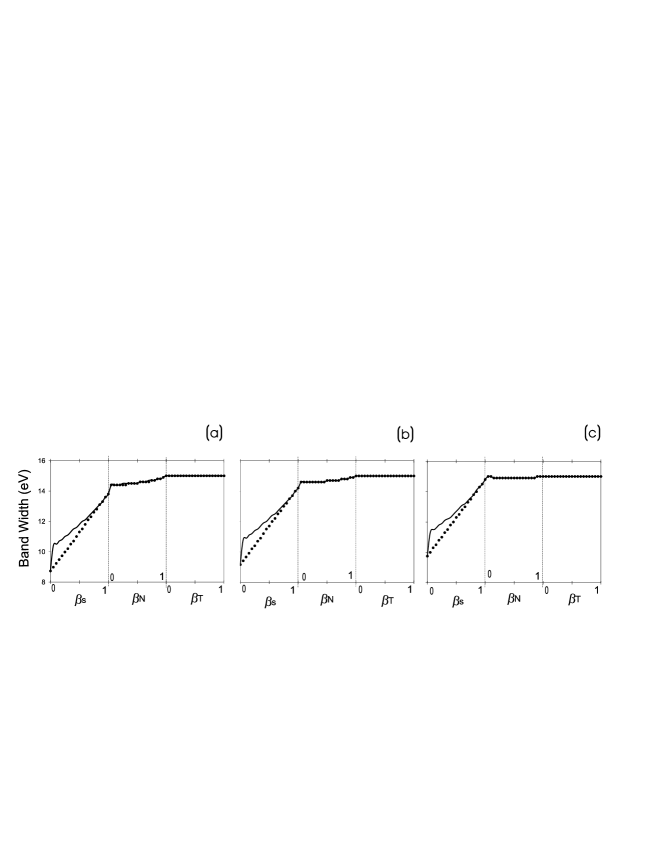
Figure 1. Band with evolution of (3,0), (4,0) and (9,0) structures both in the Harigaya’s model and in the toy model. As $\beta_{\mathrm{S}}$ varies both $\beta_{\mathrm{N}}$ and $\beta_{\mathrm{T}}$ are kept fixed at zero; as $\beta_{\mathrm{N}}$ varies $\beta_{\mathrm{S}}$ is kept fixed at 1 and $\beta_{\mathrm{T}}$ is kept fixed at zero and as $\beta_{\mathrm{T}}$ varies both $\beta_{\mathrm{S}}$ and $\beta_{\mathrm{T}}$ are kept fixed at 1. Solid and dotted lines correspond to the variations in the Harigaya’s model and in the toy model, respectively.

Next, we show band gap, i.e., the difference between HOMO and LUMO. For (3,0) the gap initiate with 3.39 eV, the gap value of trans-PA. As graphene evolves, the gap goes down almost in a parallel way for both models to 0. This is consistent of graphene being a zero-gap semiconductor whose electronic structure near the Fermi energy is given by an occupied $\pi$ band and an empty $\pi^{\ast}$ band. It is quite clear from Fig. 2(a) that in the Harigaya’s model the gap drops to zero for $t_{0}=1.63$ eV while it drops to zero for $t_{0}^{\mathrm{t,r}}=1.38$ eV in the toy model. This is due to the looseness of the constraint conditions compared to those in Harigaya’s model. At the latest stages of graphene formation and during the formation of open ended nanotube, the gap vanishes and with the beginning of nanotube with periodic boundaries it jumps up to 0.39 eV and falls to 0.33 eV at the completion when Harigaya’s model is used. Hence, according to this model we have a nonzero gap for a (3,0) nanotube. SSH model does not include bond angle and bond length variations giving rise to finite curvature effects in nanotubes, detected in several experiments as small energy gap near the Fermi level [14]. Therefore, the tiny gap near the Fermi level in (3,0) appearing according to Harigaya’s model can not be interpreted as due to curvature effects. For this an extended form of tight binding calculations to include curvature effects had to be used [15]. But according to our toy model, the gap starts and ends with 0.08 eV and 0.07 eV during the formation stage of (3,0) nanotube with periodic boundary conditions (Fig. 2(a)). For (4,0) the initial gap value is 2.89 eV, it follows almost the same decrease up to zero and then with the beginning of nanotube with periodic boundaries jumps to relatively close values, 2.23 eV in the Harigaya’s model and 2.07 in the toy model (Fig. 2(b)). Peng et al. [16] assume that this SWCNT is a semiconductor, which was predicted to have an energy gap of about 2.5 eV based on the graphene sheet model. On the other hand, some authors [5] claim that (4,0) is metallic and this discrepancy arises from the neglect of curvature effects in the graphene sheet model. As for (9,0), the gap starts from an even smaller value, 1.91 eV and then falls to zero at $t_{0}=0.88$ eV and at $t_{0}=75$ eV, respectively. At the completion of nanotube with periodic boundaries the gap goes to zero (Fig. 2(c)).

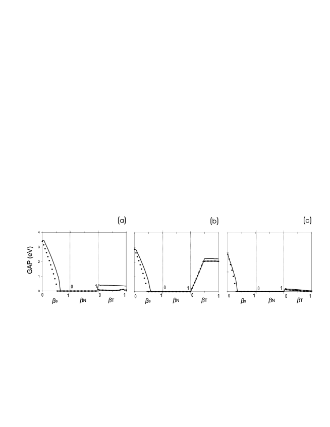
Figure 2. Band gap evolution of (3,0), (4,0) and (9,0) structures both in the Harigaya’s model and in the toy model. As $\beta_{\mathrm{S}}$ varies both $\beta_{\mathrm{N}}$ and $\beta_{\mathrm{T}}$ are kept fixed at zero; as $\beta_{\mathrm{N}}$ varies $\beta_{\mathrm{S}}$ is kept fixed at 1 and $\beta_{\mathrm{T}}$ is kept fixed at zero and as $\beta_{\mathrm{T}}$ varies both $\beta_{\mathrm{S}}$ and $\beta_{\mathrm{T}}$ are kept fixed at 1. Solid and dotted lines correspond to the variations in the Harigaya’s model and in the toy model, respectively.

We will report on calculations of one-dimensional van Hove singularities, i.e., logarithmic singularities: These singularities may be important in experimental correlations of models of nanotubes because optical absorption or emission rates in nanotubes is related primarily to the electronic states at the vHSs [17]. In this respect, the electronic transition energies $E_{ii},\,i=1,2,3,\ldots$, that is the energy separations between $i^{\mathrm{t}h}$ vHSs in the DOS of the conduction and valence bands play the fundamental role since the measured absorption peaks occur at these transition energies [18,19].

The recent progress in measuring the absorption peaks of single SWCNT instead of SWCNTs bundle is encouraging [1]. In this way effects arising from ensemble averaging and effects introduced by a composite medium are eliminated. Besides this, combined fluorescence and Raman scattering measurements on the single molecule level open up new ways to characterize SWCNTs [1]. These are among nondestructive characterization techniques of SWCNTs, the only handicap is the effects on electronic properties due to inhomogeneities in their local environments.

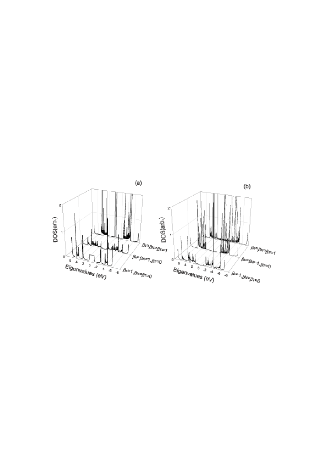
Figure 3. DOS evolution of (3,0 ) structures for K = 60. (a) for the Harigaya’s model and (b) for the toy model.

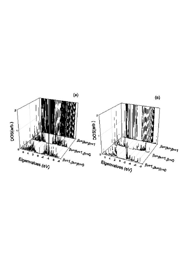
Figure 4. Same as Fig.3 but for (4,0 ).

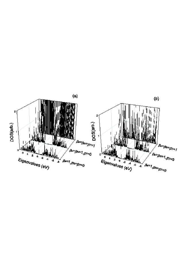
Figure 5. Same as Fig.3 and Fig.4 but for (9,0 ).

Sharp vHSs occur in carbon nanotubes with diameters less than 2 nm [6]. All of our three SWCNTs have this property, 0.235, 0.313 nm and 0.704 nm, respectively. Figs. 3, 4 and 5 respectively depict the DOS of graphene, open ended SWCNTs and nanotubes possessing periodic boundaries according to the Harigaya’s model and the toy model for (3,0), (4,0) and (9,0) structures. We calculated the energies at which these singularities appear. In the toy model the number of vHSs is higher. Gap is the interval between the first vHSs in the valance and conduction bands. For (3,0), the gap value obtained in this way is consistent with the gap value obtained from Fig.  2(b) both in the Harigaya’s model and the toy model. (4,0) has an energy gap of about 2.5 eV based on the graphene sheet model [16]. Our result is consistent with this. For (9,0), we obtain an extra van Hove singularity very close to Fermi energy according to both models. This is reasonable since (9,0) nanotubes are conducting. The next three singularities are coinciding with those of Hartschuh et al. [1].

Tubes	Models	$\beta$s	Frequencies (cm-1)
	Harigaya	$\beta_{N}=1$	25249.3
(3,0)	"	$\beta_{T}=1$	22168.4	23887.7
	Toy	$\beta_{N}=1$	19988.1	26858.3
	"	$\beta_{T}=1$	20910.7	23083.6	26941.8
	Harigaya	$\beta_{N}=1$	19881.8	24102.7	28094
(4,0)	"	$\beta_{T}=1$	19898
	Toy	$\beta_{N}=1$	20285.1	24981.5
	"	$\beta_{T}=1$	20285.1
	Harigaya	$\beta_{N}=1$	14662	20669.7	25840
(9,0)	"	$\beta_{T}=1$	11263.1	13193.4	18246.8	27226.6
	Toy	$\beta_{N}=1$	10989.6	13350	13974.8	19703.3	24117.3	25765.3
	"	$\beta_{T}=1$	11123.5	13318.4	18508.1	22206.5	23535.6	25611.1

Table 1. Calculated optical transition frequencies in both models for open ended SWCNTs and SWCNTs with periodic conditions. For the $\beta_{N}=1$ lines $\beta_{S}=1$ and $\beta_{T}=0$ and for the lines $\beta_{T}=1$ we have $\beta_{S}=\beta_{N}=1$.

Transition frequencies $\omega_{ii}=E_{ii}/\hbar$ cm^-1 in the optical spectral range for (3,0), (4,0) and (9,0) open ended nanotubes and nanotubes with periodic boundaries are selected from the calculated transition energies and are shown in Table 1.

4. Conclusion

Electronic properties, band with; band gap and vHSs of three zigzag nanotubes, (3,0) (small radius-conducting), (4,0) (semiconducting) and (9,0) (large radius-conducting) are comparatively studied in a toy model and in the Harigaya’s model. The toy model is an extension of the Harigaya’s model, it includes the contributions of bonds of different types to the SSH Hamiltonian differently. Both models give the same band width. In the (3,0) case, the band gap appearing according to the Harigaya’s model disappears when the toy model is used for periodic conditions. Both models give the same band gap for (4,0) nanotube. It agrees well with the gap value given in the literature. For (9,0) the results of both models are the same. When the toy model is used one gets many more vHSs. For (9,0) we obtained an extra singularity in the vicinity of Fermi energy. The calculated next three singularities agree with those given in the literature. We could not find any data in the literature for the correlation of the other singularities.

References

[1] Hartschuh, A.; Pedrosa, H.N.; Peterson, J.; Huang, L.; Anger, P.; Qian, H.; Meixner, A.J.; Steiner, M.; Novotny, L.; Krauss, T.D. Chem Phys Chem 2005, 6, 1.

[2] Dresselhaus, M.S.; Eklund, P.C. Advances in Phys 2000, 49, 705.

[3] Su, W.P.; Schrieffer, J.R.; Heeger, A.J. Phys Rev 1980, B22 2099.

[4] Stafstrom, S.; Riklund, R.; Chao, K.A. Phys Rev 1982, B26 4691.

[5] Cabria, I.; Mintmire, J.W.; White, C.T. Int J Quant Chem 2003, 91, 51.

[6] Harigaya, K. J Phys Soc Jpn 1991, 60, 4001.

[7] Harigaya, K. Phys Rev 1992, B45, 12071.

[8] Harigaya, K. Phys Rev 1999, B60, 1452.

[9] Harigaya, K. Synt Met 2003, 135, 751.

[10] Harigaya, K. J Phys: Condens Matter 1998, 10, 6845.

[11] Sünel, N.; Rizaoğlu, E.; Harigaya, K.; Özsoy, O. Phys Lett 2005, A338, 366.

[12] Sünel, N.; Özsoy, O. Int J Quant Chem 2004, 100, 231.

[13] Özsoy, O.; Sünel, N. Czech J Phys 2004, 54, 1495.

[14] Itkis, M.E.; Nigoyi, S.; Meng, M.E.; Hamon, M.A.; Hu, H.; Haddon, R.C. Nano Lett 2002, 2, 155.

[15] Dresselhaus, M.S.; Saito, R.; Jorio, A. Annual Review of Materials Research; August 2004; Vol. 34; Pages 247-278.

[16] Peng, L.M.; Zhang, Z.L.; Xue, Z.Q.; Wu, Q.D.; Gu, Z.N.; Pettifor, D.G. Phys Rev Lett 2000, 85, 3249.

[17] Cronin, S.B.; Swan, A.K.; Ünlü, M.S.; Goldberg, B.B.; Dresselhaus, M.S.; Tinkham, M. Phys Rev 2005, B72, 035425-1.

[18] Collins, J.E.; Sippel, J.; Arnason, S.; Rinzler, A.G. University of Florida, Department of Physics, P.O. Box 118440, Gainsesville, FL 32611-8440 U.S.A.

[19] Fantini, C.; Jorio, A.; Souza, M.; Strano, M.S.; Dresselhaus, M.S.; Pimenta, M.A. Phys Rev Lett 2004, 93, 147406-1.