Chapter 6  
The Classical Spectral Density Method
at Work: The Heisenberg Ferromagnet

Abstract

In this article we review a less known unperturbative and powerful many-body method in the framework of classical statistical mechanics and then we show how it works by means of explicit calculations for a nontrivial classical model. The formalism of two-time Green functions in classical statistical mechanics is presented in a form parallel to the well known quantum counterpart, focusing on the spectral properties which involve the important concept of spectral density. Furthermore, the general ingredients of the classical spectral density method (CSDM) are presented with insights for systematic nonperturbative approximations to study conveniently the macroscopic properties of a wide variety of classical many-body systems also involving phase transitions. The method is implemented by means of key ideas for exploring the spectrum of elementary excitations and the damping effects within a unified formalism. Then, the effectiveness of the CSDM is tested with explicit calculations for the classical $d$-dimensional spin-$S$ Heisenberg ferromagnetic model with long-range exchange interactions decaying as $r^{-p}$ ($p>d$) with distance $r$ between spins and in the presence of an external magnetic field. The analysis of the thermodynamic and critical properties, performed by means of the CSDM to the lowest order of approximation, shows clearly that nontrivial results can be obtained in a relatively simple manner already to this lower stage. The basic spectral density equations for the next higher order level are also presented and the damping of elementary spin excitations in the low temperature regime is studied. The results appear in reasonable agreement with available exact ones and Monte Carlo simulations and this supports the CSDM as a promising method of investigation in classical many-body theory.

1. Introduction

At the present a wide variety of methods exists to calculate the macroscopic equilibrium and nonequilibrium quantities of many-body systems. However, their potentialities and efficiencies differ sensibly especially when small parameters are absent for intrinsic reasons and the ordinary perturbative expansions appear inadequate. There exist, for instance, many systems of experimental and theoretical interest which involve strongly interacting microscopic degrees of freedom and exhibit anomalous behavior of the specific heat, susceptibility and other macroscopic quantities which, in turn, indicate various phase transitions to occur in these systems. Therefore, there is always a great interest to search for reliable methods going beyond the conventional perturbation theory to describe correctly nonperturbative phenomena and, especially, the various anomalies in the thermodynamic behavior of systems near a phase transition. In this connection, the two-time Green function (GF) technique constitutes one of the most powerful tools in quantum statistical mechanics and in condensed matter physics to explore the thermodynamic and transport properties of a wide variety of many-body systems. Within this framework, the equations of motion method (EMM) and the spectral density method (SDM) allow to obtain reliable approximations to treat typically nonperturbative problems [1, 2, 3, 4, 5].

When one mentions the two time GF technique, one refers usually to their quantum many-body version which is well known from long time and widely and successfully applied in quantum statistical physics. Nevertheless, the pioneering introduction of the two-time GF’s and the EMM in classical statistical mechanics by Bogoljubov and Sadovnikov [6] has opened the concrete possibility to describe classical and quantum many-body systems on the same footing. In this context, it is worth mentioning that, in many physical situations (when the quantum effects are negligible), the use of the classical two-time GF formalism may offer substantial advantages especially from the computational point of view because in the calculations one handles only functions and not operators. In any case, the strong impact of the two-time GF technique in many-body physics and the continuous efforts for obtaining better approximations are well known and, hence, it is unnecessary to stress again its effectiveness and potentialities. Rather, the less known SDM merits further remarks.

The SDM was formulated some decades ago by Kalashnikov and Fradkin for quantum many-body systems [4, 5]. It is sufficiently simple and has been applied to a wide variety of quantum systems, also exhibiting phase transitions [5], as superconductors [4, 5], magnetic [4, 5, 7] and bosonic [8] systems, strongly correlated electron compounds [5, 9, 10, 11], and so on. It appears more effective than the EMM for a direct calculation of two-time GF’s, not only because it allows to obtain reliable and systematic nonperturbative approximations, but also because it assures the validity of a number of sum rules irrespective either to the interaction strength or any other characteristics inherent to the system under study.

Next, a classical version of the SDM (CSDM) has been also formulated in extensive [12, 13, 14] and nonextensive [15] classical statistical mechanics and applied to classical magnetic systems with short and long-range exchange interactions. The last method, strictly related to the classical two-time GF technique [6], offers a robust technical instrument for systematic and well tested nonperturbative approximations to explore the equilibrium and transport properties of classical many-body systems as well, parallel to the quantum counterpart. Unfortunately, both the mentioned methods in the classical context have not received the due consideration and further developments and applications are desirable.

In this article, also with a pedagogical aim in mind, we first review the basic formalism of two-time GF’s in classical statistical mechanics in a form strictly parallel to the quantum better known counterpart emphasizing the concept of spectral density (SD), quite important for next purposes, and its relation to the two-time GF’s. Besides, as a convenient alternative to the EMM for calculation of the GF’s, the basic ingredients of the CSDM are presented in some details, together with useful insights for systematic nonperturbative approximations. Then, we clarify how this method can be conveniently used to explore macroscopic properties of classical many-body systems. We introduce also the key ideas for studying, in a conceptually transparent way, the elementary excitation spectrum, or dispersion relation, and the damping effects in a unified way within the formalism of CSDM. The general presentation of the method in the classical many-body framework will be performed in a form strictly related to the well known quantum counterpart [1, 2, 5], giving the possibility to use powerful calculation techniques, approximation methods and the basic terminology which are typical of the quantum many-body theory.

Next, we will show, with explicit calculations, how the CSDM works emphasizing its effectiveness already to the lowest order of approximation. As a nontrivial theoretical laboratory, we choose the classical $d$-dimensional spin-$S$ Heisenberg ferromagnet with long-range interactions (LRI’s), decaying as $r^{-p}$ ($p>d$) with distance $r$ between spins, in the presence of an external magnetic field. For this model, besides some partial exact results [16, 17, 18, 19, 20], a lot of new information about thermodynamic and critical properties have been obtained by means of Monte Carlo (MC) simulations [21, 22]. As we shall see, the CSDM allows us to obtain, in a relatively simple way, untrivial results which appear to be in a reasonable agreement with the available exact ones and MC simulations supporting the SDM as a promising method of investigation also in classical statistical mechanics.

The paper is organized as follows. In Sec. 2, we introduce the two-time GF’s and the related SD’s in classical statistical mechanics for two arbitrary dynamic variables. Section 3 is devoted to the methods of calculation focusing on the general formulation of the CSDM. Here, the method is properly implemented for exploring also the damping of the classical excitations within the same basic formalism. The method at work is presented in Sec. 4 with a study of the thermodynamic properties and the critical phenomena of the classical $d$-dimensional spin-$S$ Heisenberg ferromagnetic model with LRI’s. Here, after a summary of known theoretical and simulational information about the model for a next checking of the effectiveness of the CSDM, we present explicit calculations performed by using the general many-body formalism developed before. As a successive useful comparison, we first formulate the problem in the context of the EMM for the two-time GF’s appropriate to the spin model under study and the basic equations in the Tyablikov-like approximation (classical version of the well known quantum Tyablikov one [2]) are presented. Then, the basic SD and related moment equations (ME’s) are derived, the thermodynamic and critical properties of the model are presented working in the so called one-pole approximation for the SD and a comparison with the Tyablikov-like results is performed. To underline the effectiveness of this lowest order approximation and the nature of difficulties arising to higher orders, we deduce the basic equations for the two-poles approximation. As a further insight, we use the implemented CSDM to obtain, in a unified and relatively simple way, the dispersion relation and the damping of classical spin excitations. Explicit results are given (for the short-range FM chain) in the low-temperature limit. Finally, in Sec. 5 some conclusions are drawn.

2. Two-Time Green Functions and Spectral Densities
in Classical Statistical Mechanics

2.1 Basic Definitions and Spectral Representations

In strict analogy with the quantum case [1, 2, 3, 23], we define [6] the two-time retarded $(\nu=r)$ and advanced $(\nu=a)$ GF’s in classical statistical mechanics for two arbitrary dynamical variables $A$ and $B$ as

$$G_{AB}^{(\nu)}(t,t^{\prime})=\theta_{\nu}(t-t^{\prime})\left\langle\left\{A(t),B\left(t^{\prime}\right)\right\}\right\rangle\equiv\left\langle\left\langle A(t);B\left(t^{\prime}\right)\right\rangle\right\rangle_{\nu}\begin{array}[]{cc},&(\nu=r,a),\end{array}$$ (2.1)

where $\theta_{r}(t-t^{\prime})=\theta(t-t^{\prime})$, $\theta_{a}(t-t^{\prime})=-\theta(t^{\prime}-t)$ and $\theta(x)$ is the usual step function. In Eq. (2.1), $\left\langle...\right\rangle$ denotes an equilibrium or a nonequilibrium ensemble average [23] and $\left\{A,B\right\}$ is the Poisson bracket of $A$ and $B$. In the following, we refer only to the equilibrium (generalized) ensemble average. In this case one can easily prove [23] that the two-time GF’s (2.1) and the corresponding correlations functions depend on times $t$, $t^{\prime}$ only through the difference $t-t^{\prime}$. So, one can write

$$G_{AB}^{(\nu)}(t-t^{\prime})=\left\langle\left\langle A(t-t^{\prime});B\right\rangle\right\rangle_{\nu}=\left\langle\left\langle A;B(t^{\prime}-t)\right\rangle\right\rangle_{\nu}.$$ (2.2)

In the previous equations, the dynamical variables $A$ and $B$ depend on time via the conjugate canonical coordinates $(q(t),p(t))\equiv(q_{1}(t),..,q_{\mathcal{N}}(t);p_{1}(t),..,p_{\mathcal{N}}(t))$, ($\mathcal{N}$ is the number of degrees of freedom of the classical system under study), $X(t)=e^{iLt}X(0)$ with $X=A,B,q,p$, $L=i\{H,...\}$ is the Liouville operator and $H$ is the Hamiltonian. Here, $e^{iLt}$ acts as a classical time-evolution operator which transforms the dynamical variable $X(0)\equiv X(q(0),p(0))$ at the initial time $t=0$ into the dynamical variable $X(t)\equiv X(q(t),p(t))$ at the arbitrary time $t$. Of course, the time evolution of the generic dynamical variable $X(t)$ is governed by the well known Liouville equation of motion (EM)

$${\frac{{dX(t)}}{{dt}}}=\left\{{X(t),H}\right\}.$$ (2.3)

With the previous definitions, one can show [6] that the two-time correlation function $F_{AB}(t,t^{\prime})=F_{AB}(t-t^{\prime})={\left\langle A(t)B(t^{\prime})\right\rangle}={\left\langle A(\tau)B\right\rangle}={\left\langle AB(-\tau)\right\rangle}$, with $\tau=t-t^{\prime}$, is related to the classical GF’s (2.2) by the relation

$$G_{AB}^{(\nu)}(\tau)=\beta\theta_{\nu}(\tau)\frac{d}{d\tau}\left\langle{A(\tau)B}\right\rangle=\beta\theta_{\nu}(\tau)\left\langle\left\{{A(\tau),H}\right\}{B}\right\rangle,$$ (2.4)

where $\beta=\left({K_{B}T}\right)^{-1}$, $T$ is the temperature and $K_{B}$ is the Boltzmann constant. In particular, we have also

$$\left\langle{\left\{{A(\tau),B}\right\}}\right\rangle=\beta{\frac{d}{{d\tau}}}\left\langle{A(\tau)B}\right\rangle=\beta\left\langle{\left\{{A(\tau),H}\right\}B}\right\rangle,$$ (2.5)

which connects the Poisson bracket of two dynamical variables and the corresponding dynamical correlation function.

Working, as assumed before, within equilibrium Gibbs ensembles, one can introduce for $G_{AB}^{(\nu)}(\tau)$ and $F_{AB}(\tau)$ the Fourier transforms

$$G_{AB}^{(\nu)}(\tau)=\int_{-\infty}^{+\infty}{{\frac{{d\omega}}{{2\pi}}}}G_{AB}^{(\nu)}(\omega)e^{-i\omega\tau},$$ (2.6)

$$F_{AB}(\tau)=\int_{-\infty}^{+\infty}{{\frac{{d\omega}}{{2\pi}}}}F_{AB}(\omega)e^{-i\omega\tau},$$ (2.7)

where $G_{AB}^{(\nu)}(\omega)=\left\langle{\left\langle{A(\tau);B}\right\rangle}\right\rangle_{\nu,\omega}$ will be named the $\nu$-GF’s of $A$ and $B$ in the $\omega$-representation and $F_{AB}(\omega)=\left\langle{A(\tau)B}\right\rangle_{\omega}$ is called the classical spectral intensity of the time-dependent correlation function $F_{AB}(\tau)$, with $\Im(\omega)=\int_{-\infty}^{+\infty}d\tau e^{i\omega\tau}\Im(\tau)$. Then, using Eq. (2.4) and the integral representations

$$\theta(\tau)={i}\int_{-\infty}^{+\infty}\frac{{dx}}{{2\pi}}{{\frac{{e^{-ix\tau}}}{{x+i\varepsilon}}}}\begin{array}[]{ccc},&\varepsilon\rightarrow 0^{+};&\end{array}\delta(x)=\int_{-\infty}^{+\infty}\frac{{d\tau}}{{2\pi}}{e^{ix\tau},}$$ (2.8)

for the step function and the Dirac $\delta$-function, the Fourier transforms of the two-time GF (2.1) for two dynamical variables $A$ and $B$ can be expressed in terms of the corresponding spectral intensity as:

$$G_{AB}^{(\nu)}(\omega)=\int_{-\infty}^{+\infty}{{\frac{{d\omega}^{\prime}}{{2\pi}}}}{\frac{{\beta\omega}^{\prime}{F_{AB}(\omega}^{\prime}{)}}{{\omega-\omega}^{\prime}{+(-1)^{\nu}i\varepsilon}}}\quad,\quad\varepsilon\rightarrow 0^{+},$$ (2.9)

where the symbol $(-1)^{\nu}$ means $+1$ if $\nu=r$ and $-1$ if $\nu=a$. It is interesting to compare Eq. (2.9) with the quantum corresponding one for two operators $A$ and $B$ [1, 2, 3, 23]

$$G_{AB}^{(\nu)}(\omega)=\int_{-\infty}^{+\infty}{{\frac{{d\omega}^{\prime}}{{2\pi}}}}{\frac{{(1+\eta e^{-\beta\hbar\omega^{\prime}})F_{AB}(\omega}^{\prime}{)}}{{\omega-\omega}^{\prime}{+(-1)^{\nu}i\varepsilon}}}\quad,\quad\varepsilon\rightarrow 0^{+},$$ (2.10)

where $\eta=-1$ and $\eta=+1$ for definition of quantum two-time GF’s with commutator or anticommutator, respectively, and $\hbar$ is the reduced Planck constant. Notice that formally, as expected for internal consistency, the function $C(\omega)=\beta\omega$ or $Q_{\eta}(\omega)=(1+\eta e^{-\beta\hbar\omega})/\hbar$ characterizes the classical or quantum nature of the problem under study, respectively.

In analogy to the quantum case [4, 5], we now introduce the time-dependent classical spectral density (CSD) for $A$ and $B$ [12, 13, 14, 24]

$$\Lambda_{AB}(\tau)=i\left\langle{\left\{{A(\tau),B}\right\}}\right\rangle.$$ (2.11)

Taking its Fourier transform, we get

$$\Lambda_{AB}(\omega)=i\left\langle{\left\{{A(\tau),B}\right\}}\right\rangle_{\omega}=\int_{-\infty}^{+\infty}{d\tau}e^{i\omega\tau}\Lambda_{AB}(\tau)=\beta\omega F_{AB}(\omega).$$ (2.12)

Hence, from Eq. (2.9), one immediately obtains the spectral representation

$$G_{AB}^{(\nu)}(\omega)=\int_{-\infty}^{+\infty}{{\frac{{d\omega}^{\prime}}{{2\pi}}}}{\frac{{\Lambda_{AB}(\omega}^{\prime}{)}}{{\omega-\omega}^{\prime}{+(-1)^{\nu}i\varepsilon}}}\quad,\quad\varepsilon\rightarrow 0^{+},$$ (2.13)

for the two-time GF’s (2.1) in terms of the corresponding CSD $\Lambda_{AB}(\omega)$ in the $\omega$-representation. Also the dynamical correlation function $\left\langle A(\tau)B\right\rangle$ can be easily expressed in terms of $\Lambda_{AB}(\omega)$. From Eqs. (2.5), (2.11) and (2.12), we obtain indeed

$$\left\langle A(\tau)B\right\rangle=\int_{-\infty}^{+\infty}{\frac{d\omega}{2\pi}}{\frac{\Lambda_{AB}(\omega)}{\beta\omega}}e^{-i\omega\tau}.$$ (2.14)

Eqs. (2.13) and (2.14) assume a particular importance for our purposes. If one determines independently the $\Lambda_{AB}(\omega)$, these equations allow us to obtain the time-dependent correlation and Green functions and therefore the macroscopic properties of classical many-body systems. We will show below that, also in classical statistical mechanics, it is possible to construct a formalism which allows for a systematic calculation of the CSD.

From Eqs. (2.11)-(2.14) some immediate exact results can be easily obtained. First, Eqs. (2.11) and (2.12) yield

$$\int_{-\infty}^{+\infty}{{\frac{{d\omega}}{{2\pi}}}}\Lambda_{AB}(\omega)=i\left\langle{\left\{{A,B}\right\}}\right\rangle.$$ (2.15)

Besides, from (2.14), it follows

$$\int_{-\infty}^{+\infty}{{\frac{{d\omega}}{{2\pi}}}}{\frac{\Lambda_{AB}(\omega)}{\beta\omega}}=\left\langle AB\right\rangle.$$ (2.16)

The relations (2.15) and (2.16) are formally exact and constitute useful examples of the so called sum rules of the CSD, $\Lambda_{AB}(\omega)$, which have great relevance for physical consistency of practical calculations and approximations. Combining now Eqs. (2.13) and (2.15), one can easily prove another general result which plays an important role for calculation of the GF’s. As $\omega\rightarrow\infty$ we have indeed

$$G_{AB}^{(\nu)}(\omega) = \omega^{-1}\int_{-\infty}^{+\infty}{{\frac{{d\omega}^{\prime}}{{2\pi}}}}{\frac{{\Lambda_{AB}(\omega}^{\prime}{)}}{{1-{\frac{{\omega}^{\prime}{-(-1)^{\nu}i\varepsilon}}{\omega}}}}}$$

$$\approx {\frac{1}{\omega}\int_{-\infty}^{+\infty}{{\frac{{d\omega^{{}^{\prime}}}}{{2\pi}}}}\Lambda_{AB}(\omega^{{}^{\prime}})\left[{1+{\frac{{\omega}^{\prime}{-(-1)^{\nu}i\varepsilon}}{\omega}}+{\frac{1}{2}}{\frac{{\left({\omega}^{\prime}{-(-1)^{\nu}i\varepsilon}\right)^{2}}}{{\omega^{2}}}}+...}\right]}$$

$$= {\frac{{i\left\langle{\left\{{A,B}\right\}}\right\rangle}}{\omega}}+{\frac{1}{{\omega^{2}}}}\int_{-\infty}^{+\infty}{{\frac{{d\omega}^{\prime}}{{2\pi}}}}\Lambda_{AB}(\omega^{\prime})\left({\omega}^{\prime}{-(-1)^{\nu}i\varepsilon}\right)+O\left({{\frac{1}{{\omega^{3}}}}}\right).$$

So, we can write

$$G_{AB}^{(\nu)}(\omega)=\left\{\begin{array}[]{ccc}{\frac{{i\left\langle{\left\{{A,B}\right\}}\right\rangle}}{\omega}}\sim\omega^{-1}&,&if\quad\left\langle{\left\{{A,B}\right\}}\right\rangle\neq 0\\ \sim\omega^{-\alpha}\quad(\alpha\geq 2)&,&if\quad\left\langle{\left\{{A,B}\right\}}\right\rangle=0,\end{array}\right.$$ (2.18)

which provide a relevant boundary conditions for the $\nu$-GF’s.

Let’s come back now to the relations (2.13) for classical retarded and advanced GF’s in the $\omega$-representation. As in the quantum counterpart [1, 2], using the definitions (2.1) and (2.2), one can easily prove that $G_{AB}^{(r)}(\omega)$ and $G_{AB}^{(a)}(\omega)$, analytically continued in the $\omega$-complex plane, are analytical functions in the upper and lower half-plane, respectively. Then, combining these two analytical functions, one can construct a single function$G_{AB}(\omega)=\int_{-\infty}^{+\infty}dte^{i\omega t}G_{AB}(t)$ of complex $\omega$ such that

$$G_{AB}(\omega)=\left\{\begin{array}[]{ccc}G_{AB}^{(r)}(\omega)&,&\text{Im }\omega>0\\ G_{AB}^{(a)}(\omega)&,&\text{Im }\omega<0.\end{array}\right.$$ (2.19)

Hence, Eq. (2.13) yields for $G_{AB}(\omega)$ the spectral representation

$$G_{AB}(\omega)=\int_{-\infty}^{+\infty}{{\frac{{d\omega}^{\prime}}{{2\pi}}}}{\frac{\Lambda_{AB}(\omega^{\prime})}{\omega-\omega^{\prime}}}.$$ (2.20)

This function is analytical in the whole complex $\omega$-plane with a cut along the real axis where singularities for $G_{AB}(\omega)$ may occur. It is worth noting that, in terms of $\Lambda_{AB}(\omega)$, no formal differences exist for the spectral representations of $G_{AB}^{(\nu)}(\omega)$ and $G_{AB}(\omega)$ in the classical and quantum context. Hence, all the developments already known in quantum many-body theory remain formally valid for the classical case. So, one has immediately the important exact relation

$$\Lambda_{AB}(\omega)=i\left[G_{AB}(\omega+i\varepsilon)-G_{AB}(\omega-i\varepsilon)\right],$$ (2.21)

which express the CSD in terms of the related two-time GF’s in the $\omega$-representation. This allows us to state also that the cut for $G_{AB}(\omega)$ along the real axis in $\omega$-complex plane is determined by Eq. (2.21) and its singularities are the points of the real axis where the condition $\Lambda_{AB}(\omega)\neq 0$ is satisfied. For the spectral intensity of classical systems, Eqs. (2.12) and (2.21) yield

$$F_{AB}(\omega)=\left\langle{A(\tau)B}\right\rangle_{\omega}=i{\frac{{G_{AB}(\omega+i\varepsilon)-G_{AB}(\omega-i\varepsilon)}}{{\beta\omega}}.}$$ (2.22)

Of course, other known quantum relations are formally valid for classical many-body theory. For instance, when $\Lambda_{AB}(\omega)$ is real, the classical Kramer-Kronig relations (classical dispersion relations) between the real and imaginary parts of $G_{AB}^{(r)}(\omega)$ and $G_{AB}^{(a)}(\omega)$ for real values of $\omega$ are true

$$\text{Re }G_{AB}^{(\nu)}(\omega)={\frac{(-1)^{(\nu)}}{\pi}}\wp\int_{-\infty}^{+\infty}d\omega^{\prime}{\frac{\text{Im }G_{AB}^{(\nu)}(\omega^{\prime})}{\omega^{\prime}-\omega},}$$ (2.23)

where the symbol $\wp$ denotes the main part of the integral defined as

$$\wp\int_{-\infty}^{+\infty}{\frac{f(x)}{x-x_{0}}}=\lim_{\varepsilon\rightarrow 0^{+}}\left[{\int_{-\infty}^{x_{0}-\varepsilon}{dx{\frac{{f(x)}}{{x-x_{0}}}}+\int_{x_{0}+\varepsilon}^{+\infty}{{\frac{{f(x)}}{{x-x_{0}}}}}}}\right].$$ (2.24)

We have also

$$\Lambda_{AB}(\omega)=-2(-i)^{\nu}{\text{Im }G_{AB}^{(\nu)}(\omega),}$$ (2.25)

and, in particular,

$$\Lambda_{AB}(\omega)=-2{\text{Im }G_{AB}^{(r)}(\omega)}.$$ (2.26)

Many physical information about the macroscopic properties of classical many body systems can be obtained from the analytical properties of the GF’s defined above. In the Subsec. 2.2 we will derive a spectral decomposition for $\Lambda_{AB}(\omega)$, and hence for $G_{AB}^{(\nu)}(\omega)$ and $F_{AB}(\omega)$, from which it becomes possible to analyze the nature of the classical GF singularities and their connection with the physical quantities.

2.2 Spectral Decompositions, Classical Oscillations and Damping

In this section we will show that, in strict analogy with quantum case, also in classical statistical mechanics an exact spectral decomposition for the CSD is true. With this aim, following Refs. [25, 26], we introduce the Hilbert space of the classical dynamical variables with a scalar product defined as

$$\left\langle A\left|B\right.\right\rangle\overset{def}{=}Z\left\langle A^{\ast}B\right\rangle=\int{d\Gamma e^{-\beta H}A^{\ast}(q,p)B(q,p),}$$ (2.27)

where $d\Gamma=dqdp$ and $Z=\int{d\Gamma e^{-\beta H}}$ is the (generalized) partition function for the problem under study. In this space one can consider the eigenvalue equation for the Hermitian operator $L$

$$L\left|\psi_{k}\right\rangle=\omega_{k}\left|\psi_{k}\right\rangle,$$ (2.28)

or, equivalently, in terms of the wave functions $\psi_{k}(q,p)$ corresponding to the vectors $\left|\psi_{k}\right\rangle$

$$L\psi_{k}(q,p)=\omega_{k}\psi_{k}(q,p).$$ (2.29)

In Eqs. (2.28) and (2.29), $\left|\psi_{k}\right\rangle$ $\left(\psi_{k}\right)$ and $\omega_{k}$ denote the eigenvectors (eigenfunctions) and the eigenvalues of the Liouville operator $L$.

An important property of the Liouville operator is that all its eigenfunctions are (in general) complex [25] and one can promptly prove that, if $\psi_{k}$ is an eigenfunction of $L$ with eigenvalue $\omega_{k}$, then $\psi_{k}^{\ast}$ is also an eigenfunction of $L$ with eigenvalue $-\omega_{k}$.

At this stage, if we assume that $\{\psi_{k}\}$ is a complete set of orthonormal eigenfunctions ($\left\langle\psi_{k}\left|\psi_{k^{\prime}}\right.\right\rangle=Z\left\langle\psi_{k}^{\ast}(q,p)\psi_{k}(q,p)\right\rangle=\delta_{k,k^{\prime}}$), for two arbitrary dynamical variables $A(q,p)$ and $B(q,p)$ we can consider the expansions:

$$\begin{array}[]{c}A(p,q)=\sum_{k}\left\langle\psi_{k}^{\ast}\left|A\right.\right\rangle\psi_{k}^{\ast}(q,p),\\ B(p,q)=\sum_{k}\left\langle\psi_{k}\left|B\right.\right\rangle\psi_{k}(q,p).\end{array}$$ (2.30)

On the other hand, from the relations (2.5), (2.11) and (2.12), it follows that

$$\Lambda_{AB}(\omega) = \beta\omega\int_{-\infty}^{+\infty}{d\tau e^{i\omega\tau}\left\langle{A(\tau)B}\right\rangle}$$

$$= \beta\omega Z^{-1}\int d\Gamma e^{-\beta H(q,p)}{B(q,p)}\int_{-\infty}^{+\infty}d\tau e^{i(\omega+L)\tau}A(q,p).$$

Then, taking into account the definition (2.27), the expansions (2.30) and the orthonormality and completeness conditions in the Hilbert space, Eq. (2.2) yields

$$\Lambda_{AB}\left(\omega\right)=2\pi\beta\omega Z^{-1}\sum_{k}\left\langle\psi_{k}^{\ast}\left|A\right.\right\rangle\left\langle\psi_{k}\left|B\right.\right\rangle\delta(\omega-\omega_{k}),$$ (2.32)

where we have used the relations

$$e^{i(\omega+L)\tau}\psi_{k}^{*}=e^{i(\omega-\omega_{k})\tau}\psi_{k}^{\ast},$$ (2.33)

and

$$\int_{-\infty}^{+\infty}d\tau e^{i(\omega-\omega_{k})\tau}{=2\pi\delta(\omega-\omega_{k}).}$$ (2.34)

Equation (2.32) is the desired spectral decomposition, or classical Lehmann representation, for the $\Lambda_{AB}(\omega)$ to be compared with the known quantum analog [4, 5]. Of course, if $B=A^{\ast}$, we have

$$\Lambda_{AA^{\ast}}(\omega)=2\pi\beta\omega Z^{-1}\sum_{k}\left|\left\langle\psi_{k}^{\ast}\left|A\right.\right\rangle\right|^{2}\delta\left(\omega-\omega_{k}\right),$$ (2.35)

which is a real quantity. Equations (2.32) and (2.35) express formally $\Lambda_{AB}(\omega)$ as an infinite sum of appropriately weighted $\delta$-functions. It may happen that, for special physical cases, only a finite number of terms in the sum of Eqs. (2.32) and (2.35) are different from zero. In such cases, the many-body problem may be solvable. Usually, however, $\Lambda_{AB}(\omega)$ will be a continuous function of real frequency $\omega$.

It is easy to see that $\Lambda_{AB}(\omega)$ can be also written in the compact form

$$\Lambda_{AB}(\omega)=2\pi\beta\omega\left\langle{B\delta(\omega+L)A}\right\rangle=2\pi i\left\langle{\left\{{\delta(\omega+L)A,B}\right\}}\right\rangle,$$ (2.36)

which, in view of definition (2.27), is just the operatorial version of the spectral decomposition (2.32).

An important consequence of the general expression (2.32) for $\Lambda_{AB}(\omega)$ is that the $G_{AB}(\omega)$, defined by Eqs. (2.19) and (2.20), can be written as

$$G_{AB}(\omega)=\left\langle{\left\langle{A(\tau);B}\right\rangle}\right\rangle_{\omega}=\beta Z^{-1}\sum\limits_{k}{\left\langle{\psi_{k}\left|B\right.}\right\rangle\left\langle{\psi_{k}^{\ast}\left|A\right.}\right\rangle{\frac{{\omega_{k}}}{{\omega-\omega_{k}}}.}}$$ (2.37)

Hence, the eigenvalues of the Liouville operator $L=i\{H,...\}$, which is related to the energy of the system, are just the real poles of the Green function $G_{AB}(\omega)$. On the other hand, from Eq. (2.14), one has for the $\tau$-dependent correlation function $F_{AB}(\tau)$

$$F_{AB}(\tau)=\left\langle{A(\tau)B}\right\rangle=Z^{-1}\sum\limits_{k}{\left\langle{\psi_{k}\left|B\right.}\right\rangle\left\langle{\psi_{k}^{\ast}\left|A\right.}\right\rangle}e^{-i\omega_{k}\tau}.$$ (2.38)

Then, in strict analogy to the quantum case, Eqs. (2.37) and (2.38) suggest that the real poles of $G_{AB}(\omega)$, i.e. the eigenvalues $\omega_{k}$ of the Liouville operator, represent the classical frequency spectrum of undamped oscillations (elementary or collective depending on the physical nature of the dynamical variables $A$ and $B$) in the system. A characteristic frequency of this type will be called the oscillation dispersion relation. Thus, in case of polar singularities, the real poles of $G_{AB}(\omega)$ represent undamped oscillations of the system associated to the time-dependent correlation function for the dynamical variables $A$ and $B$. It is worth noting that, in general, the $\delta$-poles in the exact classical Lehmann representation (2.2) of the spectral density are expected lying infinitesimally close, therewith defining a continuous function $\Lambda_{AB}(\omega)$. It is then obvious that the damped oscillation concept works only under the basic presumption that the CSD exhibits some pronounced peaks, which have to be identified with oscillation poles for $G_{AB}(\omega)$. The widths of these peaks are a direct measure of damping and, therefore, of the finite lifetime of various quasioscillations in the system. This can still better be seen by inspecting the connection of $\Lambda_{AB}(\omega)$ with the $G_{AB}^{(r)}(\omega)$. We start from the observation that further complicated singularities may occur in the $\omega$-complex plane on the Riemann sheet of the analytical function $G_{AB}(\omega)$ below the real axis where $G_{AB}^{(r)}(\omega)$ is not an analytical function. Then, in order to see what may happen, let us assume that, in this region, at least approximately, a complex pole of the type $\tilde{\omega}_{AB}=\omega_{AB}-i\Gamma_{AB}$ ($\Gamma_{AB}>0$) may take place for $G_{AB}^{(r)}(\omega)$. In this simple situation, one can write

$$G_{AB}^{(r)}(\omega)\approx{\frac{{C_{AB}}}{{\omega-\omega_{AB}+i\Gamma_{AB}}}}$$ (2.39)

for real $\omega$ very close to the singularity value $\omega_{AB}$. In Eq. (2.39), $C_{AB}$ is an inessential constant depending on the nature of the dynamical variables $A$ and $B$. Besides, we suppose also that $\Lambda_{AB}(\omega)$ is a continuous real function of $\omega$ so that we can use the exact relation (2.26). Then, from Eq. (2.39), we obtain the (approximate) expression

$$\Lambda_{AB}(\omega)\simeq 2\frac{{\Gamma_{AB}}\text{Re }{C_{AB}-(\omega-\omega_{AB})\text{Im }C_{AB}}}{{(\omega-\omega_{AB})^{2}+\Gamma_{AB}^{2}}}.$$ (2.40)

If $\Lambda_{AB}(\omega)>0$, we should have necessarily $\text{Im }C_{AB}=0$ and hence $\Lambda_{AB}(\omega)$ should have a Lorentzian shape. Unfortunately, according to the exact spectral decompositions (2.32) and (2.36), $\Lambda_{AB}(\omega)$ is not a definite positive function in the whole range of real $\omega$. Hence, in principle, for each polar singularity for $G_{AB}^{(r)}(\omega)$ one must assume the quasi-Lorentzian or modified Lorentzian expression (2.40) which reduces to a $\delta$-function singularity for $\omega$ close to $\omega_{AB}$ and $\Gamma_{AB}\rightarrow 0$. In any case, using the representation (2.8) for $\theta(\tau)$, from Eq. (2.39) and the inverse Fourier transform for $G_{AB}^{(r)}(\omega)$, the time behavior of the retarded GF is given by

$$G_{AB}^{(r)}(\tau)=\theta(\tau)\left\langle{\left\{{A(\tau),B}\right\}}\right\rangle\approx\theta(\tau)\mathcal{A}_{AB}(\tau)e^{-i\omega_{AB}\cdot\tau},$$ (2.41)

where

$$\mathcal{A}_{AB}(\tau)=\mathcal{A}_{AB}e^{-\Gamma_{AB}\cdot\tau},$$ (2.42)

with $\mathcal{A}_{AB}$ an inessential constant. Similarly, using the exact relation (2.5) and the approximate expression for $\left\langle\left\{{A(\tau),B}\right\}\right\rangle$ which can be extracted from Eq. (2.41), one easily finds:

$$\left\langle{A(\tau)B}\right\rangle-\left\langle A\right\rangle\left\langle B\right\rangle\simeq\mathcal{C}_{AB}(\tau)e^{-i\omega_{AB}\tau}=(\mathcal{C}_{AB}e^{-\Gamma_{AB}\tau})e^{-i\omega_{AB}\tau}.$$ (2.43)

Eq. (2.43) is based on the boundary condition $\mathop{\lim}\limits_{\tau\rightarrow\infty}\left\langle{A(\tau)B}\right\rangle=\left\langle A\right\rangle\left\langle B\right\rangle$ related to the physical feature that, for all real systems, there is always attenuation of the correlations on time. This is also supported by the rigorous Riemann-Lebesgue lemma in theory of analytical functions [23] as applied to the spectral representation (2.7) where the spectral intensity $F_{AB}(\omega)$, and hence $\Lambda_{AB}(\omega)$, is a continuous function.

In conclusion, when $G_{AB}^{(r)}(\omega)$ has a pole below the real axis, with $\omega$ close to $\omega_{AB}$ and $\Gamma_{AB}/\left|{\omega_{AB}}\right|\ll 1$, $\Lambda_{AB}(\omega)$ has a pronounced quasi-Lorentzian peak at $\omega=\omega_{AB}$ and both $G_{AB}^{(r)}(\omega)$ and $\left\langle{A(\tau)B}\right\rangle-\left\langle A\right\rangle\left\langle B\right\rangle$ are characterized by damped oscillations with frequency $\omega_{AB}$. Here $\Gamma_{AB}$, which is related to the width of the peak, measures the damping of oscillations. Of course, in this picture, $\tau_{AB}=\Gamma_{AB}^{-1}$ defines the life-time of the oscillations in the system. It is also worth noting that, if $\Gamma_{AB}=0$ (absence of damping), $\Lambda_{AB}(\omega)$ has a $\delta$-function peak and undamped oscillations with frequency $\omega_{AB}$ occur in the system.

The considerations made above for a single pole for $G_{AB}^{(r)}(\omega)$ very close the real $\omega$-axis from below can be easily extended to several singularities of this type. In such a case, $\Lambda_{AB}(\omega)$ will result in a superposition of modified Lorentzian peaks whose widths measure the damping of the related oscillations. If the widths reduce to zero, $\Lambda_{AB}(\omega)$ becomes a superposition of $\delta$-functions and this signals the occurrence of undamped oscillations in the system.

In the next section, where we will consider the problem to search reliable approximations within the classical GF formalism, we will see that the quasi-Lorentzian shape for $\Lambda_{AB}(\omega)$ is not mathematically adequate and another more appropriate representation, capturing the essential physics, will be necessary.

3. Methods of Calculation

All the previous general considerations suggest that, also in classical statistical mechanics, the formalism of the two-time GF’s may be a useful tool to study the macroscopic properties of classical many-body systems. The basic ingredients are $G_{AB}(\omega)$ and $\Lambda_{AB}(\omega)$ for two properly chosen dynamical variables $A$ and $B$. Remarkably, if we are able to calculate $G_{AB}(\omega)$ $(\Lambda_{AB}(\omega))$, the exact relations established in the previous sections allow us to obtain $\Lambda_{AB}(\omega)$ $(G_{AB}(\omega))$. In the present section we present the classical formulation of two general methods in strict analogy to the quantum counterpart, i.e. the classical EMM, for calculating the GF’s, and the CSDM for a direct calculation of the SD. In principle, both the methods should give exactly the GF’s and the related SD’s and hence, in this sense, they are completely equivalent. Nevertheless, in practical calculations, previous experiences in quantum many-body theory [4, 5, 7, 8, 9, 10, 11, 12] and, although reduced, in classical many-body theory [12, 13, 14, 15, 22, 27], suggest that the SDM has several advantages to make more reliable nonperturbative approximations in a systematic and controllable manner.

3.1 The Classical Equations of Motion Method

Differentiating Eq. (2.2) with respect to $\tau=t-t^{{}^{\prime}}$ yields

$$\frac{d}{d\tau}\left\langle{\left\langle{A(\tau);B}\right\rangle}\right\rangle_{\nu}={\frac{{d\theta_{\nu}(\tau)}}{{d\tau}}}\left\langle{\left\{{A(\tau),B}\right\}}\right\rangle+\left\langle{\left\langle{{\frac{{dA(\tau)}}{{d\tau}}};B}\right\rangle}\right\rangle_{\nu}.$$ (3.1)

Then, using the EM (2.3) for dynamical variables and the obvious relation $d\theta_{\nu}(\tau)/d\tau=\delta(\tau)$, Eq. (3.1) becomes

$${\frac{d}{{d\tau}}}\left\langle{\left\langle{A(\tau);B}\right\rangle}\right\rangle_{\nu}=\delta(\tau)\left\langle{\left\{{A,B}\right\}}\right\rangle+\left\langle{\left\langle{\left\{{A(\tau),H}\right\};B}\right\rangle}\right\rangle_{\nu}.$$ (3.2)

This is the basic EM for the GF $\left\langle{\left\langle{A(\tau);B}\right\rangle}\right\rangle_{\nu}$ which, however, is not a closed differential equation. Indeed, in the right-hand side of Eq. (3.2) a new higher order $\nu$-GF occurs involving Poisson brackets of a greater number of dynamical variables. Then, one needs to consider a new EM for the two-time $\nu$-GF $\left\langle{\left\langle{\left\{{A(\tau),H}\right\};B}\right\rangle}\right\rangle_{\nu}$. The $\tau$-derivative of this function yields an additional equation, formally identical to Eq. (3.2) with $A(\tau)$ replaced by ${\left\{{A(\tau),H}\right\}}$, the right-hand side of which contains the new $\nu$-GF $\left\langle{\left\langle\left\{{\left\{{A(\tau),H}\right\},H}\right\}{;B}\right\rangle}\right\rangle_{\nu}$. By iteration of this procedure, we obtain an infinite chain of coupled EM’s for GF’s of increasing order which can be written in a compact form as

$$\frac{d}{d\tau}\left\langle{\left\langle{\mathcal{L}_{H}^{m}A(\tau);B}\right\rangle}\right\rangle_{\nu}=\delta(\tau)\left\langle{\left\{{\mathcal{L}_{H}^{m}A,B}\right\}}\right\rangle+\left\langle{\left\langle{\mathcal{L}_{H}^{m+1}A(\tau);B}\right\rangle}\right\rangle_{\nu}\begin{array}[]{cc},&(m=0,1,2,...).\end{array}$$ (3.3)

Here $\mathcal{L}_{H}=iL=\{...,H\}$ and $\mathcal{L}_{H}^{m}A$ means $\mathcal{L}_{H}^{0}A=A$, $\mathcal{L}_{H}^{1}=\{A,H\}$, $\mathcal{L}_{H}^{2}A=\{\{A,H\},H\}$, and so on. Notice that the chain of EM’s (3.3) is formally the same for different types of GF’s and hence one can eliminate the index $\nu$ when the physical context is clear.

In the practical calculations it is generally more convenient to work in the $\omega$-Fourier space. With $i\int_{-\infty}^{+\infty}d\tau e^{i\omega\tau}\left(d{f(\tau)/d\tau}\right)=\omega f(\omega)$, the chain of equations, in the $\omega$-representation, assumes the form:

$$\omega\left\langle{\left\langle{\mathcal{L}_{H}^{m}A(\tau);B}\right\rangle}\right\rangle_{\nu,\omega}=i\left\langle{\left\{{\mathcal{L}_{H}^{m}A,B}\right\}}\right\rangle+i\left\langle{\left\langle{\mathcal{L}_{H}^{m+1}A(\tau);B}\right\rangle}\right\rangle_{\nu,\omega}\begin{array}[]{cc},&(m=0,1,2,...).\end{array}$$ (3.4)

To solve the chain of EM’s in the form (3.3) or (3.4), we must add appropriate boundary conditions. For this, it is again more convenient to use the $\omega$-representation (3.4) for which they can be obtained in the form of spectral representations or dispersion relations for the GF’s (see Subsec. 2.1 and, in particular, Eq. (2.18)), in strict analogy with the quantum case. Anyway, although Eqs. (3.3) and (3.4) are exact, a free solution for interacting systems is, of course, impossible. In practical calculations one is forced to introduce decoupling procedures, and hence approximate methods, to reduce the infinite chain of coupled equations in a finite closed one which, although approximate, may be solved. However, in general, systematic and controllable decouplings are not easy to find and one must check the reliability of a given approximation by comparing the results with experiments, simulations or other types of approaches. The CSDM, which will be the subject of the next subsection, seems more flexible in such a direction.

3.2 The Classical Spectral Density Method

Here, we present a general formulation of the CSDM [12, 14] for a systematic calculation of the CSD. For this aim, it is convenient to start from the expression (2.11) of the SD in the $\tau$-representation. By successive derivatives of ${\Lambda_{AB}(\tau)}$ with respect to $\tau$ and using the EM (2.3), one has

$${\frac{{d^{m}\Lambda_{AB}(\tau)}}{{d\tau^{m}}}=}i\left\langle{\left\{{\mathcal{L}_{H}^{m}A(\tau),B}\right\}}\right\rangle\begin{array}[]{cc},&(m=0,1,2,...).\end{array}$$ (3.5)

Then, taking the Fourier transform of Eq. (3.5), we easily get

$$(-i\omega)^{m}\Lambda_{AB}(\omega)=i\int_{-\infty}^{+\infty}d\tau e^{i\omega\tau}\left\langle\left\{{\mathcal{L}_{H}^{m}A(\tau),B}\right\}\right\rangle.$$ (3.6)

Finally, integration over $\omega$ yields:

$$\int_{-\infty}^{+\infty}{{\frac{{d\omega}}{{2\pi}}}\omega^{m}\Lambda_{AB}(\omega)=-i^{m-1}\left\langle{\left\{\mathcal{L}{{}_{H}^{m}A,B}\right\}}\right\rangle}\begin{array}[]{cc},&(m=0,1,2,...).\end{array}$$ (3.7)

The quantity on the left-hand side of Eq. (3.7) is called the m-moment of $\Lambda_{AB}(\omega)$ and the relations (3.7) constitute an infinite set of exact ME’s or sum rules for the CSD. Notice that, for $m=0$, the sum rule (2.15) is reproduced.

Equations (3.7) can be seen in a different way. Indeed, since the Poisson brackets and hence the ensemble averages involved in the right-hand side of relations (3.7) can be evaluated, at least in principle, it is quite remarkable that the $m$-moments of the SD can be explicitly obtained without the a priori knowledge of the function $\Lambda_{AB}(\omega)$. This important result implies that the sequence of Eqs. (3.7) represents a typical moment problem. Its solution would yield the unknown SD and hence all the related quantities (GF’s, correlation functions and other observables). Unfortunately, also this problem, in general, cannot be solved exactly and one must look for an approximate solution. Suggested by the exact classical spectral decomposition (2.32) or (2.35), we seek for an approximation for $\Lambda_{AB}(\omega)$ as a finite sum of properly weighted $\delta$-functions of the form (polar approximation)

$$\Lambda_{AB}(\omega)=2\pi\sum\limits_{k=1}^{n}{\lambda_{k}(A,B)\delta\left({(\omega-\omega_{k}(A,B)}\right),}$$ (3.8)

where $n$ is a finite integer number. The unknown parameters $\lambda_{k}(A,B)$ and $\omega_{k}(A,B)$, depending on the nature of the dynamical variables A and B, have to be determined as a solution of the finite set of $2n$ (generally integral) equations obtained by inserting the expression (3.8) in the first $2n$ ME’s (3.7). This is the basic idea of the CSDM. Physically, the parameters $\omega_{k}(A,B)$ in Eq. (3.8) play the role of effective eigenvalues of the Liouville operator and each of them, as a real (approximate) pole of the GF $G_{AB}(\omega)$ (see the spectral representation (2.20) or (2.37)), corresponds to a possible mode of undamped oscillations for the correlation function $\left\langle A(\tau)B\right\rangle$ (see Eq. (2.38)).

As discussed at the end of Sec. 2, there are physical situations where the damping of classical oscillations in the system under study may be important and hence the polar approximation (3.8) is inadequate. In these cases, the basic idea of the SDM, related to the moment problem (3.7), remains still valid but it is necessary to chose a more appropriate functional structure for the SD which allows us to determine the modes of oscillations in the system and their damping or life-time. An extension of the SDM in this sense was first proposed by Nolting and Oles [28] for Fermi systems and by Campana et al. [13] for Bose and classical systems whose SD’s are not positive definite in the whole range of $\omega$. Here we will focus on the classical case. In Sec. 2, we have shown that information about the spectrum and the damping of the oscillations in the system can be obtained if the SD is assumed as a superposition of the quasi-Lorentzian peaks. The peaks would correspond to the frequencies of oscillations and the widths would measure their damping or life-time. However, we are now in a position to easily check that modified Lorentzian shapes for $\Lambda_{AB}(\omega)$ cannot be valid over the whole $\omega$ range since all the SD moments of order $m\geq 2$ would diverge. This feature clearly contradicts Eq. (3.7). To assure the convergency of the SD moments at any order and to preserve the intrinsic physical character of the CSD’s connected with the not everywhere-positive factor $\omega$ in the exact spectral decomposition (2.32) or (2.35), one can assume the modified Gaussian ansatz for the $\Lambda_{AB}(\omega)$ [13]

$$\Lambda_{AB}(\omega)=2\pi\omega\sum\limits_{k=1}^{n}{\lambda_{k}(A,B){\frac{{\exp\left[{{\frac{{-\left({\omega-\omega_{k}(AB)}\right)^{2}}}{{\Gamma_{k}(A,B)}}}}\right]}}{\sqrt{\pi\Gamma_{k}(A,B)}}}.}$$ (3.9)

Notice that, with the functional representation (3.9) for $\Lambda_{AB}(\omega)$, the parameter ${\Gamma_{k}(A,B)}$ has not to be identified directly with the parameter ${\Gamma(A,B)}$ in Eqs. (2.39) for $G_{AB}(\omega)$ and (2.40) for $\Lambda_{AB}(\omega)$ but, rather, with ${\Gamma}^{2}{(A,B)}$. Then, the width of the peak in $\omega=\omega_{k}(A,B)$ is represented here by ${\Gamma_{k}^{1/2}(A,B)}$, the condition ${\Gamma(A,B)/\left|{\omega(A,B)}\right|}\ll 1$ must be replaced by ${\Gamma_{k}(A,B)/\left[{\omega_{k}(A,B)}\right]^{2}}\ll 1$ and the life-time of the classical excitations with frequency $\omega_{k}(A,B)$ is identified by $\tau_{k}(A,B)={\Gamma_{k}^{1/2}(A,B)}$. The choose (3.9) is only motivated by the fact that it takes direct contact with the notation used in literature [13, 28] and simplifies the algebra in explicit calculations. Here the parameters $\omega_{k}(A,B)$ represent the oscillation frequencies and the new parameters $\Gamma_{k}(A,B)$, which describe the broadening of the $\delta$-poles due to the finite life-times of the respective oscillations, give a measure of the damping effects. In any case, the representation (3.9) assures that $\Lambda_{AB}(\omega)$ is a superposition of sharp quasi-$\delta$-function peaks and reduces to the polar one (3.8) in the limit $\Gamma_{k}(A,B)\rightarrow 0$, as expected. This functional structure allows us to investigate classical oscillations and damping effects systematically just as the $\delta$-function ansatz (3.8) does for case of undamped oscillations. Of course, with the ansatz (3.9), the parameters $\lambda_{k}(A,B)$, $\omega_{k}(A,B)$ and $\Gamma_{k}(A,B)$ have to be calculated solving the first $3n$ ME’s (3.7) consistently with the basic condition ${\Gamma_{k}(A,B)/\left[{\omega_{k}(A,B)}\right]^{2}}\ll 1$.

As in the EMM, also in the SDM the problem remains to close the truncated finite set of ME’s arising from the polar ansatz (3.8) or the modified Gaussian ansatz (3.9). In any case, the evaluation of the right-hand sides of Eqs. (3.7) generally involves higher order SD’s. Therefore, higher order moment problems should be considered, but the difficulty of calculations will increase considerably. So, in order to solve self-consistently the finite set of ME’s, which arises from Eq. (3.7) using the ansatz (3.8) or (3.9), it is usually necessary to use some decoupling procedures and thus to introduce, in a systematic way, additional approximations in the CSDM which, however, will be automatically consistent with an increasing number of sum rules for the SD.

4. The Classical $d$-dimensional Spin-$S$ Heisenberg Ferromagnet with Long-Range Interactions: A Many-body Approach

4.1 An Introduction to the Model

The classical $d$-dimensional spin-$S$ Heisenberg ferromagnet with LRI’s decaying as $r^{-p}$ ($p>d$) with the distance $r$ between spins, in the presence of an external magnetic field, is described by the Hamiltonian

$$H=-{\frac{1}{2}}\sum\limits_{i,j=1}^{N}{J_{ij}\vec{S}_{i}\cdot\vec{S}_{j}}-h\sum\limits_{i=1}^{N}{S_{i}^{z}}.$$ (4.1)

Here $N$ is the number of sites of a hypercubic lattice with unitary spacing,$\left\{{\vec{S}_{j}\equiv(S_{j}^{x},S_{j}^{y},S_{j}^{z});}\text{ }{j=1,...,N}\right\}$ are the classical spins, $h$ is the external magnetic field and the exchange interaction, in view of the thermodynamic limits as $N\rightarrow\infty$, is assumed to be $J_{ij}=J/r_{ij}^{p}$, where $r_{ij}=\left|{\vec{r}_{i}-\vec{r}_{j}}\right|$ and $J$ measures the strength of the spin-spin coupling. The extreme case $p\rightarrow\infty$ corresponds to the standard nearest-neighbor interaction while the mean field approximation is obtained when $p=0$ (replacing $J$ by $J/N$). For this type of interaction, the thermodynamic limit $N\rightarrow\infty$ is well defined only for $p>d$, while for $p\leq d$ the ground state of the system has an infinite energy per spin as $N\rightarrow\infty$ and the conventional statistical mechanics cannot be directly applied.

The classical spin model (4.1) can be properly described by the set of $2N$ canonical variables $\{\varphi_{j},S_{j}^{z}\}$ where $\varphi_{j}$ is the angle between the projection of the spin vector $\vec{S}_{j}$ in the $(x-y)$-plane and the $x$-axis. The Poisson bracket of two arbitrary classical dynamical variables $A(\varphi,S^{z})$ and $B(\varphi,S^{z})$ is then defined by

$$\left\{{A,B}\right\}=\sum\limits_{j=1}^{N}{\left({{\frac{{\partial A}}{{\partial\varphi_{j}}}}{\frac{{\partial B}}{{\partial S_{j}^{z}}}}-{\frac{{\partial A}}{{\partial S_{j}^{z}}}}{\frac{{\partial B}}{{\partial\varphi_{j}}}}}\right)}.$$ (4.2)

For the following calculations, we find convenient to introduce the new spin variables $S_{j}^{\pm}=S_{j}^{x}\pm iS_{j}^{y}$, so that $S^{2}=(S_{j}^{z})^{2}+S_{j}^{+}S_{j}^{-}.$ Then, if one defines the Fourier transforms of the spin vectors and the exchange interaction as

$$\vec{S}_{\vec{k}}=\sum\limits_{j=1}^{N}{e^{-i\vec{k}\cdot\vec{r}_{j}}\vec{S}_{j}}\quad,\quad J(\vec{k})=\sum\limits_{j=1}^{N}{e^{-i\vec{k}\cdot(\vec{r}_{i}-\vec{r}_{j})}J_{ij},}$$ (4.3)

where $\vec{k}$ denotes a wave vector in the $d$-dimensional Fourier space, the Hamiltonian (4.1) can be rewritten as (with ${J(\vec{k})=J(-\vec{k})}$)

$$H=-{\frac{1}{{2N}}}\sum\limits_{\vec{k}}{J(\vec{k})\left({S_{\vec{k}}^{+}S_{-\vec{k}}^{-}+S_{\vec{k}}^{z}S_{-\vec{k}}^{z}}\right)}-hS_{0}^{z}.$$ (4.4)

The sum in Eq. (4.4) is restricted to the first Brillouin zone ($1BZ$) of the lattice. Within this representation, the Poisson brackets for the spin Fourier components relevant for us are

$$\left\{{S_{\vec{k}}^{\pm},S_{k^{\prime}}^{z}}\right\}=\pm iS_{\vec{k}+\vec{k}^{\prime}}^{\pm}\quad,\quad\left\{{S_{\vec{k}}^{+},S_{k^{\prime}}^{-}}\right\}=-2iS_{\vec{k}+\vec{k}^{\prime}}^{z}.$$ (4.5)

On the basis of the previous definitions, it is now easy to establish exact general formulas for the internal energy and the free energy per spin from which all the thermodynamic properties of the spin model (4.1) can be obtained when the appropriate GF’s or SD’s have been determined using the many-body formalism presented before. For this aim, the Fourier representation (4.4) of the Hamiltonian in terms of the dynamical variables $S_{\vec{k}}^{+}S_{-\vec{k}}^{-}$ and $S_{\vec{k}}^{z}S_{-\vec{k}}^{z}$ is particularly convenient since, in general, all the thermodynamic quantities can be easily expressed exactly in terms of the correlation functions $\left\langle S_{\vec{k}}^{+}S_{-\vec{k}}^{-}\right\rangle$ and $\left\langle S_{\vec{k}}^{z}S_{-\vec{k}}^{z}\right\rangle$. To see this, we rewrite Eq. (4.2) as :

$$H=H_{0}+H_{I}(J),$$ (4.6)

with

$$H_{0}=-hS_{0}^{z},$$ (4.7)

and

$$H_{I}(J)=-{\frac{J}{{2N}}}\sum\limits_{\vec{k}}{\gamma(}\vec{k})\left[{S_{\vec{k}}^{+}S_{-\vec{k}}^{-}+S_{\vec{k}}^{z}S_{-\vec{k}}^{z}}\right],$$ (4.8)

where $\gamma(\vec{k})=J({\vec{k}})/J=\sum\limits_{j=1}^{N}{e^{i\vec{k}\cdot(\vec{r}_{i}-\vec{r}_{j})}/r_{ij}^{p}}$. Then, the internal energy of the spin model is formally given by the ensemble average

$$U=U_{0}(J)+U_{I}(J),$$ (4.9)

where

$$U_{0}(J)=\left\langle H_{0}\right\rangle=-h\left\langle S_{0}^{z}\right\rangle,$$ (4.10)

and

$$U_{I}(J)=\left\langle{H_{I}}\right\rangle\left(J\right)=-{\frac{J}{{2N}}}\sum\limits_{\vec{k}}{\gamma(}\vec{k})\left[{\left\langle{S_{\vec{k}}^{+}S_{-\vec{k}}^{-}}\right\rangle+\left\langle{S_{\vec{k}}^{z}S_{-\vec{k}}^{z}}\right\rangle}\right].$$ (4.11)

For the free energy $F=-\beta^{-1}\text{ln}Z$, we have

$${\frac{{\partial F}}{{\partial J}}}={\frac{1}{Z}}\int{d\Gamma}\left({{\frac{{\partial H_{I}(J)}}{{\partial J}}}}\right)e^{-\beta H}=\left\langle{{\frac{{\partial H_{I}(J)}}{{\partial J}}}}\right\rangle=\left\langle{{\frac{{H_{I}(J)}}{J}}}\right\rangle.$$ (4.12)

Then, by integrating Eq. (4.12) between $0$ and $J$ with the initial condition $F(J=0)=F_{0}=-\beta^{-1}\text{ln}\left[{\int d\Gamma e^{-\beta{H_{0}}}}\right]$, we get

$$F=F_{0}+\int_{0}^{J}{{\frac{{dJ^{\prime}}}{{J^{\prime}}}}\left\langle{H_{I}}\right\rangle(J^{\prime}).}$$ (4.13)

From these general expressions, it is easy to obtain, for the internal energy $u=U/N$ and the free energy $f=F/N$ per spin, the desired exact relations (with $N\rightarrow\infty$)

$$u(T,h)={\frac{{\left\langle H\right\rangle}}{N}}=-{\frac{h}{N}}\left\langle{S_{0}^{z}}\right\rangle-{\frac{J}{{2N^{2}}}}\sum\limits_{\vec{k}}{\gamma(\vec{k})\left[{\left\langle{S_{\vec{k}}^{+}S_{-\vec{k}}^{-}}\right\rangle+\left\langle{S_{\vec{k}}^{z}S_{-\vec{k}}^{z}}\right\rangle}\right]},$$ (4.14)

and

$$f(T,h) = f_{0}+{\frac{1}{N}}\int_{0}^{J}{{\frac{{dJ^{\prime}}}{{J^{\prime}}}}\left\langle{H_{I}}\right\rangle}(J^{\prime})$$

$$= f_{0}+{\frac{1}{{2N^{2}}}}\sum\limits_{\vec{k}}{\gamma(\vec{k})\int_{0}^{J}{dJ^{\prime}}\left[{\left\langle{S_{\vec{k}}^{+}S_{-\vec{k}}^{-}}\right\rangle_{J^{\prime}}+\left\langle{S_{\vec{k}}^{z}S_{-\vec{k}}^{z}}\right\rangle_{J^{\prime}}}\right]}.$$

Here, $f_{0}$ is the free energy per spin for a magnetic model without interactions and $\left\langle{...}\right\rangle_{J^{\prime}}$ denotes an ensemble average as function of the interaction strength $J^{\prime}$. So, when the correlation functions $\left\langle S_{\vec{k}}^{+}S_{-\vec{k}}^{-}\right\rangle$ and $\left\langle S_{\vec{k}}^{z}S_{-\vec{k}}^{z}\right\rangle$ are known, Eqs. (4.14) and (4.1) allow us to determine $u$ an $f$ and hence all the thermodynamic quantities using standard relations.

Also the transverse $(\xi_{\perp})$ and longitudinal $(\xi_{z})$ correlation lengths can be obtained in terms of the previous exact relations. This can be performed by using the definitions

$$\xi_{\perp}^{2}=-{\frac{1}{2}}\mathop{\lim}\limits_{k\rightarrow 0}\left\{\frac{1}{{\left\langle{S_{\vec{k}}^{+}S_{-\vec{k}}^{-}}\right\rangle}}{{\frac{d^{2}}{{dk^{2}}}}}\left\langle{S_{\vec{k}}^{+}S_{-\vec{k}}^{-}}\right\rangle\right\}$$ (4.16)

and

$$\xi_{z}^{2}=-{\frac{1}{2}}\mathop{\lim}\limits_{k\rightarrow 0}\left\{{{\frac{1}{{\left\langle{S_{\vec{k}}^{z}S_{-\vec{k}}^{z}}\right\rangle}}\frac{d^{2}}{{dk^{2}}}}\left\langle{S_{\vec{k}}^{z}S_{-\vec{k}}^{z}}\right\rangle}\right\}.$$ (4.17)

It is worth nothing that, since the SDM allows to calculate $\left\langle S_{\vec{k}}^{+}S_{-\vec{k}}^{-}\right\rangle$ and $\left\langle S_{\vec{k}}^{z}S_{-\vec{k}}^{z}\right\rangle$ solving integral ME’s, all the thermodynamic quantities can be obtained without the explicit calculation of the partition function. This is a relevant aspect of the SDM as a moment problem both in quantum and classical statistical mechanics.

As a conclusion of this subsection, to fully appreciate the effectiveness of the CSDM, it may be useful to summarize the main known features about the model (4.1)-(4.4) obtained by means of rigorous methods, MC simulations and alternative microscopic techniques. For a future comparison, we include also some information for the corresponding quantum spin model which attracted recently much interest.

The one and two dimensional long-range quantum spin-$1/2$ Heisenberg ferromagnets (for brevity reasons, models of the type (4.1) will be also named long-range spin models) in absence of an external magnetic field were investigated by Nakano and Takahashi using the so called modified spin-wave theory [29] and the Schwinger-boson mean field approximation [30]. Further information were derived for the $d$-dimensional case by means of the EMM for the two-time GF’s using the Tyablikov decoupling procedure [31] (in the next section we will present shortly the corresponding classical version for model (4.1)). Monte Carlo simulations for the two-dimensional quantum spin-$1/2$ Heisenberg model have been performed for $2<p\leq 6$ [32]. This scenario has been recently enriched by an extension [20] of the Mermin-Wagner theorem [33] for the existence of ferromagnetic (FM) long-range order (LRO) at finite temperature in quantum Heisenberg and $XY$ models in $d$($=1,2$) dimensions with $r^{-p}-$ and oscillating$-$ exchange interactions.

Classical long-range spin-$S$ Heisenberg FM models have attracted great attention, too. It has been rigorously proved the LRO exists in d(=1,2) dimension when $d<p<2d$ [16, 17] and is destroyed at all finite temperatures for $p\geq 2d$ [18, 19]. Similar results were obtained for the spherical model [34] and the present scenario of the critical properties is largely based on renormalization group calculations for the classical $n$-vector model [35, 36]. Classical long-range antiferromagnetic (AFM) models have been studied less extensively. The available rigorous results [16, 17, 18] suggest orientational disorder at all finite temperatures when $p\geq 2d$, but no theorem exists entailing existence or absence of LRO for $d<p<2d$. Monte Carlo simulations have been also performed for both $d$($=1,2$)-dimensional classical FM (for $p=2d$ [21]) and AFM (for $p={\frac{3}{2}}$ and $p=1$ with $d=1$ and $d=2$, respectively [22]) Heisenberg long-range models. The results confirm that FM-LRO survives at finite temperature provided $d<p<2d$ and allow to conjecture that no AFM-LRO exists at all finite temperatures for $p>d$. Spin-wave studies [22] agree with the last conjecture but no definitive statement can be drawn at the present stage.

Recent studies for model (4.1) [24, 27] via the CSDM to lowest order approximation are in good agreement with previous available analytical and numerical investigations. Below we present the problem in a detailed and more systematic way with the inclusion of additional results showing the efficiency of the SDM also in classical statistical mechanics. In next subsection, as mentioned before, we present also the essential results for the model (4.1) using the classical EMM and the Tyablikov-like approximation, although our main interest is devoted to the CSDM which will be used extensively in the remaining part of the article. In any case, these results will be very useful as a comparison and to underline the potentiality of the classical many-body formalism presented in Secs. 2 and 3.

4.2 The Classical Equations of Motion Method and the Tyablikov-Like
Approximation

For the Hamiltonian model in the form (4.4), we introduce the GF (without distinction between the retarded and advanced one)

$$G_{\vec{k}}(t-t^{\prime})=\left\langle{\left\langle{S_{\vec{k}}^{+}(t);S_{-\vec{k}}^{-}(t^{\prime})}\right\rangle}\right\rangle,$$ (4.18)

with the Fourier transform

$$G_{\vec{k}}(\omega)=\left\langle{\left\langle{S_{\vec{k}}^{+}(\tau);S_{-\vec{k}}^{-}}\right\rangle}\right\rangle_{\omega}=\int_{-\infty}^{+\infty}d\tau G_{\vec{k}}(\tau)e^{i\omega\tau}.$$ (4.19)

From Eq. (3.2), we have for $G_{\vec{k}}(\omega)$ the EM

$$\omega G_{\vec{k}}(\omega)=i\left\langle{\left\{{S_{\vec{k}}^{+},S_{-\vec{k}}^{-}}\right\}}\right\rangle+i\left\langle{\left\langle{\left\{{S_{\vec{k}}^{+}(\tau),H}\right\};S_{-\vec{k}}^{-}}\right\rangle}\right\rangle_{\omega}.$$ (4.20)

Then, using the spin Poisson brackets (4.5), Eq. (4.20) reduces to

$$(\omega-h)G_{\vec{k}}(\omega)=2Nm+$$

$$-{\frac{1}{N}}\sum\limits_{\vec{p}}{J(\vec{p})}\left\{{\left\langle{\left\langle{S_{\vec{k}-\vec{p}}^{z}(\tau)S_{\vec{p}}^{+}(\tau);S_{-\vec{k}}^{-}}\right\rangle}\right\rangle_{\omega}-\left\langle{\left\langle{S_{\vec{p}}^{z}(\tau)S_{\vec{k}-\vec{p}}^{+}(\tau);S_{-\vec{k}}^{-}}\right\rangle}\right\rangle_{\omega}}\right\},$$

where $m=\left\langle S_{j}^{z}\right\rangle$ is the magnetization per spin. This equation, as explained in Subsec. 3.1, is not closed and hence a decoupling procedure is necessary to determine $G_{\vec{k}}(\omega)$. In strict analogy with the quantum Tyablikov decoupling [2], we introduce the classical Tyablikov-like decoupling (or random phase like approximation) for which one can approximate

$$\begin{array}[]{c}\left\langle{\left\langle{S_{\vec{k}-\vec{p}}^{z}(\tau)S_{\vec{p}}^{+}(\tau);S_{-\vec{k}}^{-}}\right\rangle}\right\rangle_{\omega}\simeq\left\langle{S_{\vec{k}-\vec{p}}^{z}}\right\rangle\left\langle{\left\langle{S_{\vec{p}}^{+}(\tau);S_{-\vec{k}}^{-}}\right\rangle}\right\rangle_{\omega},\\ \left\langle{\left\langle{S_{\vec{p}}^{z}(\tau)S_{\vec{k}-\vec{p}}^{+}(\tau);S_{-\vec{k}}^{-}}\right\rangle}\right\rangle_{\omega}\simeq\left\langle{S_{\vec{p}}^{z}}\right\rangle\left\langle{\left\langle{S_{\vec{k}-\vec{p}}^{+}(\tau);S_{-\vec{k}}^{-}}\right\rangle}\right\rangle_{\omega}.\end{array}$$ (4.22)

Then, Eq. (4.2) yields for $G_{\vec{k}}(\omega)$ the closed equation

$$(\omega-h)G_{\vec{k}}(\omega)=2Nm+m\left({J(0)-J(\vec{k})}\right)G_{\vec{k}}(\omega).$$ (4.23)

This gives ($(Ty)$ stands for Tyablikov):

$$G_{\vec{k}}^{(Ty)}(\omega)=\frac{2Nm}{\omega-\omega_{\vec{k}}^{(Ty)}}\text{ },$$ (4.24)

where

$$\omega_{\vec{k}}^{(Ty)}=h+mJ\left({\gamma(0)-\gamma(\vec{k})}\right),$$ (4.25)

is the Tyablikov-like dispersion relation. From Eq. (4.24) and the $\delta$-function representation

$$\mathop{\lim}\limits_{\varepsilon\rightarrow 0^{+}}{\frac{1}{{2\pi i}}}\left[{{\frac{1}{{x-i\varepsilon}}}-{\frac{1}{{x+i\varepsilon}}}}\right]=\delta(x),$$ (4.26)

one immediately has (see Eq. (4.2))

$$\Lambda_{k}^{(Ty)}(\omega)=i\left[{G_{\vec{k}}(\omega+i\varepsilon)-G_{\vec{k}}(\omega-i\varepsilon)}\right]=2\pi(2Nm)\delta(\omega-\omega_{\vec{k}}^{(Ty)}).$$ (4.27)

Notice that the expression (4.27) for the spectral density $\Lambda_{k}^{(Ty)}(\omega)$ satisfies the sum rule (see Eq. (2.15))

$$\int_{-\infty}^{+\infty}\frac{{d\omega}}{{2\pi}}\Lambda_{\vec{k}}^{(Ty)}(\omega){=i\left\langle{\left\{{S_{\vec{k}}^{+},S_{-\vec{k}}^{-}}\right\}}\right\rangle}=2Nm.$$ (4.28)

Finally, from the spectral representation (2.14), we find the time-dependent correlation function $\left\langle{S_{\vec{k}}^{+}(\tau)S_{-\vec{k}}^{-}}\right\rangle$ to be (hereafter we put $K_{B}=1$)

$$\left\langle{S_{\vec{k}}^{+}(\tau)S_{-\vec{k}}^{-}}\right\rangle^{(Ty)}=T\int_{-\infty}^{+\infty}{{\frac{{d\omega}}{{2\pi}}}}{\frac{{\Lambda_{\vec{k}}^{(Ty)}(\omega)}}{\omega}}e^{-i\omega\tau}={\frac{{2NmT}}{{\omega_{\vec{k}}^{(Ty)}}}}e^{-i\omega_{\vec{k}}^{(Ty)}\tau}.$$ (4.29)

In the static case ($\tau=0$), one has $\left\langle{S_{\vec{k}}^{+}S_{-\vec{k}}^{-}}\right\rangle^{(Ty)}=2NmT/\omega_{\vec{k}}^{(Ty)}$.

The previous relations contain the unknown mean value $m=\left\langle S^{z}\right\rangle$ and hence, in order to determine the thermodynamic properties of our spin model, we must obtain a suitable expression for $m$. This constitutes a serious difficulty for classical spin systems because one cannot write, also for $S=1/2$, a classical counterpart of the quantum kinematic rule for the $z$-component of the spin. However, working in the low-temperature regime where the angular momentum is nearly saturated $(S_{j}^{z}\simeq S)$, from the identity $S^{2}=(S_{j}^{z})^{2}+S_{j}^{+}S_{j}^{-}$ we have $\left|S_{j}^{+}S_{j}^{-}\right|/S^{2}\ll 1$ and the magnetization per spin $m$ can be approximately expressed in the form

$$m\simeq S-{\frac{1}{{2S}}}\left\langle{S_{j}^{+}S_{j}^{-}}\right\rangle=S-{\frac{1}{{N^{2}}}}\sum\limits_{\vec{k}}{{\frac{{\left\langle{S_{\vec{k}}^{+}S_{-\vec{k}}^{-}}\right\rangle}}{{2S}}.}}$$ (4.30)

Then, from Eq. (4.29), one should have:

$$m\simeq S\left\{{1-}\frac{Tm}{S^{2}N}{\sum\limits_{\vec{k}}}\frac{1}{\omega_{\vec{k}}^{(Ty)}}\right\}.$$ (4.31)

Equations (4.25) and (4.31) constitute a closed self-consistent system for ($\omega_{\vec{k}}^{(Ty)},m$) which can be solved to obtain the thermodynamic properties under near saturation condition.

A general and reliable expression for $m$ in terms of the dispersion relation, valid for arbitrary temperature and including the near saturation expression (4.31), was suggested in Refs. [14, 24]. However, since our main purpose is to focus on the CSDM predictions, we postpone the derivation of such general expression to the next subsection. Then, working to the lowest order in the CSDM, we will obtain a self-consistent system of equations which differs from that in the Tyablikov-like approximation only for a new expression of $\omega_{\vec{k}}$. Hence, once these more general equations are studied, one can similarly discuss the classical Tyablikov ones simply replacing $\omega_{\vec{k}}$ with $\omega_{\vec{k}}^{(Ty)}$.

4.3 The Classical Spectral Density Method and the Moment Equations

Let us introduce the $\omega$-dependent CSD

$$\Lambda_{\vec{k}}(\omega)=i\left\langle{\left\{{S_{\vec{k}}^{+}(\tau),S_{-\vec{k}}^{-}}\right\}}\right\rangle_{\omega}=i\int_{-\infty}^{+\infty}d\tau e^{i\omega\tau}\left\langle{\left\{{S_{\vec{k}}^{+}(\tau),S_{-\vec{k}}^{-}}\right\}}\right\rangle.$$ (4.32)

The system of ME’s for $\Lambda_{\vec{k}}(\omega)$, with $A=S_{\vec{k}}^{+}$ and $B=S_{-{\vec{k}}}^{-}$ in Eq. (3.7), is given by

$$\int_{-\infty}^{+\infty}{{\frac{{d\omega}}{{2\pi}}}\omega^{m}\Lambda_{\vec{k}}(\omega)=-i^{m-1}}\left\langle{\left\{{\mathcal{L}_{H}^{m}S_{\vec{k}}^{+},S_{-\vec{k}}^{-}}\right\}}\right\rangle\begin{array}[]{cc},&(m=0,1,2,...).\end{array}$$ (4.33)

Focusing on the first three ME’s for next considerations, the use of the basic Poisson brackets (4.5) yields

$$\int_{-\infty}^{+\infty}{{\frac{{d\omega}}{{2\pi}}}\Lambda_{\vec{k}}(\omega)=i}\left\langle{\left\{{S_{\vec{k}}^{+},S_{-\vec{k}}^{-}}\right\}}\right\rangle=2Nm,$$ (4.34)

$$\int_{-\infty}^{+\infty}{{\frac{{d\omega}}{{2\pi}}}\omega\Lambda_{\vec{k}}(\omega)=-}\left\langle{\left\{{\left\{{S_{\vec{k}}^{+},H}\right\},S_{-\vec{k}}^{-}}\right\}}\right\rangle$$

$$= {\frac{1}{N}}\sum\limits_{\vec{k}}{\left[{J(\vec{k}^{\prime})-J(\vec{k}-\vec{k}^{\prime})}\right]}\left({\left\langle{S_{\vec{k}^{\prime}}^{+}S_{-\vec{k}^{\prime}}^{-}}\right\rangle+2\left\langle{S_{\vec{k}^{\prime}}^{z}S_{-\vec{k}^{\prime}}^{z}}\right\rangle}\right)+2Nmh,$$

$$\int_{-\infty}^{+\infty}{{\frac{{d\omega}}{{2\pi}}}\omega^{2}\Lambda_{\vec{k}}(\omega)=-}i\left\langle{\left\{{\left\{{\left\{{S_{\vec{k}}^{+},H}\right\},H}\right\},S_{-\vec{k}}^{-}}\right\}}\right\rangle=$$

$$= {\frac{1}{{N^{2}}}}\sum\limits_{\vec{k}_{1},\vec{k}_{2}}{\left[{J(\vec{k}_{1})-J(\vec{k}_{1}+\vec{k})}\right]}\left[{J(\vec{k}_{1}-\vec{k}_{2})-J(\vec{k}_{2})}\right]\times$$

$$\left\{\left\langle{S_{\vec{k}_{2}-\vec{k}_{1}}^{+}S_{-\vec{k}_{2}}^{-}S_{\vec{k}_{1}}^{z}}\right\rangle-\left\langle{S_{\vec{k}_{2}-\vec{k}_{1}}^{+}S_{-\vec{k}-\vec{k}_{2}}^{-}S_{\vec{k}+\vec{k}_{1}}^{z}}\right\rangle-\left\langle{S_{\vec{k}_{2}-\vec{k}_{1}}^{+}S_{\vec{k}_{1}}^{-}S_{-\vec{k}_{2}}^{z}}\right\rangle+\right.$$

$$+\left.\left\langle{S_{\vec{k}+\vec{k}_{1}}^{+}S_{-\vec{k}_{2}}^{-}S_{\vec{k}_{2}-\vec{k}_{1}-\vec{k}}^{z}}\right\rangle+2\left\langle{S_{\vec{k}+\vec{k}_{1}}^{z}S_{-\vec{k}_{2}}^{z}S_{\vec{k}_{2}-\vec{k}_{1}-\vec{k}}^{z}}\right\rangle\right\}+$$

$$+{\frac{{2h}}{N}}\sum\limits_{\vec{k}_{1}}{\left[{J(\vec{k}_{1})-J(\vec{k}_{1}-\vec{k})}\right]}\left\{{\left\langle{S_{\vec{k}_{1}}^{+}S_{-\vec{k}_{1}}^{-}}\right\rangle+2\left\langle{S_{\vec{k}_{1}}^{z}S_{-\vec{k}_{1}}^{z}}\right\rangle}\right\}+2h^{2}Nm,$$

where we have made frequent use of the standard properties of the Poisson brackets.

Notice that, in view of the general Eq. (2.16), in the previous ME’s only the correlation function $\left\langle S_{\vec{k}}^{+}S_{-\vec{k}}^{-}\right\rangle$ can be exactly expressed in terms of ${\Lambda_{\vec{k}}(\omega)}$ as

$$\left\langle S_{\vec{k}}^{+}S_{-\vec{k}}^{-}\right\rangle=\int_{-\infty}^{+\infty}\frac{{d\omega}}{{2\pi}}\frac{\Lambda_{\vec{k}}(\omega)}{\beta\omega}.$$ (4.37)

As explained in Subsec. 3.2, in order to give an approximate solution to the “moment problem“ (4.33) (or (4.34)-(4.3)), according to the CSDM one must choose an appropriate functional structure for the SD. The aim is to truncate the system of moments (4.33) at different levels and to determine $\Lambda_{\vec{k}}(\omega)$ as a solution of a finite set of equations. In the next sections we will consider some of the numerous possibilities suggested in Subsec. 3.2. Although the chooses are very simple in order to avoid prohibitive calculations, they are able to capture the essential physics of the spin model under study. In any case, one must remember that finding $\Lambda_{\vec{k}}(\omega)$ as a solution of a finite set of ME’s means to have a SD which satisfies two or more sum rules.

4.3.1 One $\delta$-function Polar Ansatz

As suggested by the exact spectral decomposition (2.35), according to the spirit of the CSDM, we try to determine $\Lambda_{\vec{k}}(\omega)$, to the lowest order, in the form [13, 24, 27]

$$\Lambda_{\vec{k}}(\omega)=2\pi\lambda_{\vec{k}}\delta(\omega-\omega_{\vec{k}}),$$ (4.38)

involving two unknown parameters $\lambda_{\vec{k}}$ and $\omega_{\vec{k}}$. Then, to determine these parameters only the first two ME’s (4.34) and (4.3) are necessary. Taking into account the polar ansatz (4.38), these reduce to the integral equations:

$$\lambda_{\vec{k}} = 2Nm$$ (4.39)

$$\lambda_{\vec{k}}\omega_{\vec{k}} = 2Nmh+\frac{1}{N}\sum\limits_{\vec{k}^{\prime}}\left[J(\vec{k}^{\prime})-J(\vec{k}-\vec{k}^{\prime})\right]\left({\left\langle{S_{\vec{k}^{\prime}}^{+}S_{-\vec{k}^{\prime}}^{-}}\right\rangle+2\left\langle{S_{\vec{k}^{\prime}}^{z}S_{-\vec{k}^{\prime}}^{z}}\right\rangle}\right).$$

To close this system, we must express the involved unknown quantities in terms of $\Lambda_{\vec{k}}(\omega)$. The transverse correlation function ${\left\langle{S_{\vec{k}}^{+}S_{-\vec{k}}^{-}}\right\rangle}$, which enters the right-hand side of Eq. (LABEL:Eq4.37c), can easily expressed in terms of the SD and hence in terms of the parameters $\lambda_{\vec{k}}$ and $\omega_{\vec{k}}$. Indeed, Eq. (2.16) and the ansatz (4.38) yield

$${\left\langle{S_{\vec{k}}^{+}S_{-\vec{k}}^{-}}\right\rangle}={\frac{2Nm}{\beta\omega_{\vec{k}}}}.$$ (4.41)

Unfortunately, there is not a simple way to express the longitudinal correlation function ${\left\langle{S_{\vec{k}}^{z}S_{-\vec{k}}^{z}}\right\rangle}$ in terms of $\Lambda_{\vec{k}}(\omega)$. Hence, to close the truncated system of ME’s (4.34)-(4.3), one should introduce the longitudinal SD $\Lambda_{\vec{k}}^{(z)}({\vec{\omega}})=i\left\langle{\left\{{S_{\vec{k}}^{z}(\tau),S_{-\vec{k}}^{z}}\right\}}\right\rangle$ and then formulate and solve another moment problem according to the basic idea of the CSDM. However, this problem would be coupled to that for the transverse SD $\Lambda_{\vec{k}}(\omega)$ and the difficulties would be sensibly amplified also if a one $\delta$-function structure for both $\Lambda_{\vec{k}}(\omega)$ and $\Lambda_{\vec{k}}^{(z)}(\omega)$ is assumed. The simplest way to overcome this difficulty, frequently used in literature [4, 5, 7, 8, 9, 10, 11, 12, 13, 14, 15], is to resort, as a first level, to the decoupling procedure $\left\langle\ S_{\vec{k}}^{z}S_{-\vec{k}}^{z}\right\rangle\simeq\left\langle S_{\vec{k}}^{z}\right\rangle\left\langle S_{-\vec{k}}^{z}\right\rangle=N^{2}m^{2}\delta_{\vec{k},0}$ which corresponds to neglect the correlations between the Fourier transforms of the longitudinal spin components. With this approximation, Eqs. (4.39)-(4.41) immediately yield the self-consistent equation for the frequency dispersion relation

$$\omega_{\vec{k}}=h+m\left(J(0)-J(\vec{k})\right)+\frac{T}{N}\sum\limits_{\vec{k}^{\prime}}\frac{J(\vec{k}^{\prime})-J(\vec{k}-\vec{k}^{\prime})}{\omega_{\vec{k}^{\prime}}}{.}$$ (4.42)

It is worth noting that the first two terms in the right-hand side of Eq. (4.42) constitutes just the expression for the dispersion relation obtained in Subsec. 4.2 using the Tyablikov-like decoupling within the EMM. Of course, the previous decoupling and the Eq. (4.42) are appropriate to describe only thermodynamic regimes with a finite magnetization as under near saturation conditions. In particular, one cannot use the basic Eq. (4.42) to explore near-zero magnetization domains in the phase diagram as the critical region and the paramagnetic phase in zero external magnetic field. To overcome this difficulty, one is forced to find a more appropriate decoupling procedure for the longitudinal correlation function which allows us to obtain self-consistent ME’s appropriate for describing regimes when $m\rightarrow 0$ and preserves also the simplicity of the one $\delta$-function ansatz for the transverse SD. A possible and successful solution to this crucial question was suggested many years ago for Heisenberg spin models with short-range interactions (SRI’s) [14]. It was shown that a suitable decoupling procedure when the magnetization approaches to zero (see also Refs. [4, 37] for the quantum counterpart) consists in writing in the ME (4.3)

$$\frac{1}{N}\sum\limits_{\vec{k}^{\prime}}{\left[{J(\vec{k}^{\prime})-J(\vec{k}-\vec{k}^{\prime})}\right]\left\langle{S_{\vec{k}^{\prime}}^{z}S_{-\vec{k}^{\prime}}^{z}}\right\rangle}\simeq$$

$$\simeq \frac{1}{N}\sum\limits_{\vec{k}^{\prime}}{\left[{J(\vec{k}^{\prime})-J(\vec{k}-\vec{k}^{\prime})}\right]}\left\{{\left\langle{S_{\vec{k}^{\prime}}^{z}}\right\rangle\left\langle{S_{-\vec{k}^{\prime}}^{z}}\right\rangle-{\frac{1}{2}}\left({1-{\frac{{\left\langle{S_{0}^{z}}\right\rangle}}{{N^{2}S^{2}}}}}\right)\left\langle{S_{\vec{k}^{\prime}}^{+}S_{-\vec{k}^{\prime}}^{-}}\right\rangle}\right\}.$$

This equation only involves $\Lambda_{\vec{k}}(\omega)$ (see Eqs. (2.16) and (4.41)) and hence, inserting in the ME (4.3) one finds, for the dispersion relation, the new expression

$$\omega_{\vec{k}}=h+m\left({J(0)-J(\vec{k})}\right)+\frac{m^{2}}{S^{2}}\frac{T}{N}\sum\limits_{\vec{k}^{\prime}}\frac{J(\vec{k}^{\prime})-J(\vec{k}-\vec{k}^{\prime})}{{\omega_{\vec{k}^{\prime}}}}.$$ (4.44)

Notice that the effect of the decoupling (4.3.1) corresponds essentially to perform in Eq. (4.42) the transformation $\sum\limits_{\vec{k}^{\prime}}(...)\rightarrow m^{2}/S^{2}\sum\limits_{\vec{k}^{\prime}}(...)$. Of course, alternative decoupling procedures can be conjectured for taking into account the effect of the longitudinal spin correlations working in terms of the single $\Lambda_{\vec{k}}(\omega)$. An example, appropriate to near saturation regimes, will be presented in Subsec. 4.5.2.

4.3.2 Magnetization per Spin in Terms of the Transverse Spectral Density

To close the system of ME’s (4.34)-(4.3) for $\Lambda_{\vec{k}}(\omega)$ (and also the EM (4.2) for $G_{\vec{k}}(\omega)$), we must find an explicit expression for $m=\left\langle S_{j}^{z}\right\rangle$ in terms of the SD. A reliable and successful expression of $m$, valid for any $T$ and $h$, can be obtained by means of the following procedure within the spirit of the SDM [14, 24]. Let us introduce the higher-order SD:

$$\Omega(\omega)={\frac{1}{{N^{2}}}}\sum\limits_{\vec{k},\vec{k}^{\prime}}{\left[{i\left\langle{\left\{{S_{\vec{k}+\vec{k}^{\prime}}^{+}(\tau),S_{-\vec{k}}^{-}S_{-\vec{k}^{\prime}}^{z}}\right\}}\right\rangle_{\omega}}\right],}$$ (4.45)

where the summand is constructed by $\Lambda_{\vec{k}}(\omega)=i\left\langle{\left\{{S_{\vec{k}}^{+}(\tau),S_{-\vec{k}}^{-}}\right\}}\right\rangle_{\omega}$ with the change $S_{\vec{k}}^{+}(\tau)\rightarrow S_{\vec{k}+\vec{k}^{\prime}}^{+}(\tau)$ and $S_{-\vec{k}}^{-}\rightarrow S_{-\vec{k}}^{-}S_{-\vec{k}^{\prime}}^{z}$. The SD (4.45) is associated to the higher-order GF

$$G^{(r)}(\omega)=\sum\limits_{\vec{k},\vec{k}^{\prime}}{\left[{\theta(\tau)\left\langle{\left\{{S_{\vec{k}+\vec{k}^{\prime}}^{+}(\tau),S_{-\vec{k}}^{-}S_{-\vec{k}^{\prime}}^{z}}\right\}}\right\rangle_{\omega}}\right].}$$ (4.46)

We now perform in Eq. (4.45) the decoupling procedure

$$\left\langle{\left\{{S_{\vec{k}+\vec{k}^{\prime}}^{+}(\tau),S_{-\vec{k}}^{-}S_{-\vec{k}^{\prime}}^{z}}\right\}}\right\rangle_{\omega}\approx\left\langle{S_{-\vec{k}^{\prime}}^{z}}\right\rangle(1+a)\left\langle{\left\{{S_{\vec{k}+\vec{k}^{\prime}}^{+}(\tau),S_{-\vec{k}}^{-}}\right\}}\right\rangle,$$ (4.47)

where $a$ is an unknown parameter to be properly determined (notice that, with $a=0$, Eq. (4.47) reduces to a Tyblikov-like decoupling). It is easy to see that this allows us to reduce $\Omega(\omega)$ to the simplest form

$$\Omega(\omega)=m(1+a){\frac{1}{N}}\sum\limits_{\vec{k}}{\Lambda_{\vec{k}}(\omega),}$$ (4.48)

in terms of the original $\Lambda_{\vec{k}}(\omega)$. The parameter $a$ can be now determined by imposing a sum rule for $\Omega(\omega)$, and precisely, by requiring that the zeroth-ME for the exact $\Omega(\omega)$ is preserved in the decoupling procedure. Taking into account the general Eq. (2.15) and the identity $(S_{j}^{z})^{2}=S^{2}-S_{j}^{+}S_{j}^{-}$, a straightforward use of the Poisson bracket properties yields, for $\Omega(\omega)$ in Eq. (4.45),

$$\int_{-\infty}^{+\infty}{{\frac{{d\omega}}{{2\pi}}}\Omega(\omega)={\frac{1}{N^{2}}}\sum\limits_{\vec{k},\vec{k}^{\prime}}{\left[{i\left\langle{\left\{{S_{\vec{k}+\vec{k}^{\prime}}^{+}(\tau),S_{-\vec{k}}^{-}S_{-\vec{k}^{\prime}}^{z}}\right\}}\right\rangle}\right]=2N^{2}S^{2}-3N\left\langle{S_{j}^{+}S_{j}^{-}}\right\rangle}}.$$ (4.49)

On the other hand, the zeroth-ME for the reduced form (4.48) for $\Omega(\omega)$ is given by (see Eq. (4.34))

$$\int_{-\infty}^{+\infty}{{\frac{{d\omega}}{{2\pi}}}\Omega(\omega)\approx m(1+a){\frac{1}{N}}\sum\limits_{\vec{k}}{\int_{-\infty}^{+\infty}{{\frac{{d\omega}}{{2\pi}}}}}}\Lambda_{\vec{k}}(\omega)=2Nm^{2}(1+a).$$ (4.50)

Then, by imposing that Eqs. (4.49) and (4.50) coincide, we obtain

$$m^{2}(1+a)=S^{2}-{\frac{3}{2}}\left\langle{S_{j}^{+}S_{j}^{-}}\right\rangle.$$ (4.51)

From this equation, it follows that in the high-temperature regime, when $m\rightarrow 0$, the isotropy condition $\left\langle{S_{j}^{+}S_{j}^{-}}\right\rangle={3}S^{2}/2$ is consistently reproduced regardless of the value of $a$. On the other hand, in the regimes where the spins $S_{j}^{z}$ are nearly saturated ($S_{j}^{z}\simeq S$ or $\left|S_{j}^{+}S_{j}^{-}\right|/S^{2}\ll 1$), the magnetization per spin can be approximately expressed in the form (4.30). Then, according to Eq. (4.51), the parameter $a$ must go to zero in an appropriate way so that Eq. (4.30) is recovered. Bearing this in mind, a direct comparison between Eqs. (4.30) and (4.51) provides for $a$ the expression

$$a={\frac{{\left\langle{S_{j}^{+}S_{j}^{-}}\right\rangle}}{{2S^{2}}}.}$$ (4.52)

Inserting it in Eq. (4.51) leads to the required formula for the magnetization per spin $m$ suitable for our aims (with $h>0$)

$$m=S\left[{{\frac{{\displaystyle{1-{\frac{3}{2}}{\frac{{\left\langle{S_{j}^{+}S_{j}^{-}}\right\rangle}}{{S^{2}}}}}}}{\displaystyle{{1-{\frac{1}{2}}{\frac{{\left\langle{S_{j}^{+}S_{j}^{-}}\right\rangle}}{{S^{2}}}}}}}}}\right]^{{\frac{1}{2}}},$$ (4.53)

where

$$\left\langle{S_{j}^{+}S_{j}^{-}}\right\rangle={\frac{1}{{N^{2}}}}\sum\limits_{\vec{k}}{\left\langle{S_{\vec{k}}^{+}S_{-\vec{k}}^{-}}\right\rangle}.$$ (4.54)

One can immediately check that, under near saturation condition, Eq. (4.53) reproduces the relation (4.30). In view of Eq. (4.54) and the exact expression of ${\left\langle{S_{\vec{k}}^{+}S_{-\vec{k}}^{-}}\right\rangle}$ in terms of $\Lambda_{\vec{k}}(\omega)$ (see Eq. (4.37)), Eq. (4.53) for $m$ allows us to take immediate contact with the SDM and, in particular, with the one $\delta$-function for $\Lambda_{\vec{k}}(\omega)$ introduced in the previous subsection.

Postponing this problem to the next subsection, we wish to outline here how the expression (4.53), which is valid for arbitrary temperature and magnetic field, can be used in the EMM for $G_{\vec{k}}(\omega)$ within the Tyablikov-like approximation (see Subsec. 4.2). In this case the GF has a real pole at $\omega_{\vec{k}}^{(Ty)}=h+mJ(\gamma(0)-\gamma({\vec{k}})$ which corresponds to a one $\delta$-function for the SD. This feature and the general expression (4.53) for $m$ allows us to express $m$ as a function of $\omega_{\vec{k}}^{(Ty)}$ yielding to a system of two self-consistent equations. When this system is solved, all the thermodynamic properties can be obtained.

It is worth emphasizing that the one $\delta$-pole ansatz for $\Lambda_{\vec{k}}(\omega)$ within the CSDM, involving two ME’s, is not equivalent to the classical Tyablikov decoupling. This becomes clear by comparing the two different expressions (4.25) and (4.42) for the dispersion relation, although one assumes the same expression (4.53) (or (4.28)) for $m$. The main reason is that, while $\Lambda_{\vec{k}}^{(Ty)}(\omega)$ (and hence $\omega_{\vec{k}}^{(Ty)}$) satisfies only the first of the sum rules (4.34)-(4.3), $\Lambda_{\vec{k}}(\omega)$ (and hence $\omega_{\vec{k}}$) is obtained to satisfy both the sum rules (4.34) and (4.3). In this sense, one can claim that the one $\delta$-function ME’s solution for $\Lambda_{\vec{k}}(\omega)$ in the CSDM is better than the corresponding one derived by means of the Tyablikov-like decoupling in the classical EMM for $G_{\vec{k}}(\omega)$ and constitutes a one step beyond such an approximation.

4.3.3 Moment Equations and Dispersion Relation for one $\delta$-pole Ansatz

We now come back to the Subsec. 4.3.1 and add, to the Eq. (4.42) or (4.44) for the dispersion relation, the corresponding equation for $m$ in terms of the parameter $\lambda_{\vec{k}}$ and $\omega_{\vec{k}}$ in $\Lambda_{\vec{k}}(\omega)=\lambda_{\vec{k}}\delta(\omega-\omega_{\vec{k}})$. From Eq. (4.53), we easily have

$${\frac{{m^{2}}}{{S^{2}}}}={\frac{{1-3\displaystyle{{\frac{{Tm}}{{S^{2}N}}}\sum\limits_{\vec{k}}{{\frac{1}{{\omega_{\vec{k}}}}}}}}}{{1-\displaystyle{{\frac{{Tm}}{{S^{2}N}}}\sum\limits_{\vec{k}}{{\frac{1}{{\omega_{\vec{k}}}}}}}}},}$$ (4.55)

which, in the near saturation regime, reduces to

$$m\simeq S\left\{{1-{\frac{{Tm}}{{S^{2}N}}}\sum\limits_{\vec{k}}{{\frac{1}{{\omega_{\vec{k}}}}}}}\right\}.$$ (4.56)

Eq. (4.42) (for $m\neq 0$) or (4.44) (for $m\rightarrow 0$) and Eq. (4.55) represent the closed system of ME’s to be solved self-consistently. For this purpose it is convenient to introduce the dimensionless variables

$$\sigma={\frac{m}{S}}\quad,\quad\bar{T}={\frac{{T}}{{JS^{2}}}}\quad,\quad\bar{h}={\frac{h}{{JS}}}\quad,\quad\bar{\omega}_{\vec{k}}={\frac{{\omega_{\vec{k}}}}{{JS}}}.$$ (4.57)

Then, taking the thermodynamic limit $N\rightarrow\infty$ with ${\frac{1}{N}}\sum\limits_{\vec{k}}(...)\rightarrow\int_{1BZ}d^{d}k(...)/(2\pi)^{d}$, our self-constistent equations can be written as

$$\bar{\omega}_{\vec{k}} = \bar{h}+\sigma\Omega^{(P)}(\vec{k})R(\vec{k})$$ (4.58)

$$\sigma^{2} = {\frac{{1-3\displaystyle{\bar{T}\sigma\int_{1BZ}{{\frac{{d^{d}k}}{{(2\pi)^{d}}}}{\frac{1}{{\bar{\omega}_{\vec{k}}}}}}}}}{{1-3\displaystyle{\bar{T}\sigma\int_{1BZ}{{\frac{{d^{d}k}}{{(2\pi)^{d}}}}{\frac{1}{{\bar{\omega}_{\vec{k}}}}}}}}}}\text{ },$$ (4.59)

with

$$R({\vec{k}})=\left\{\begin{array}[]{lcl}1+{\frac{{\bar{T}}}{\sigma}}\displaystyle{\int_{1BZ}{{\frac{{d^{d}k^{\prime}}}{{(2\pi)^{d}}}}{\frac{{\Omega^{(p)}(\vec{k}-\vec{k}^{\prime})-\Omega^{(p)}(\vec{k}^{\prime})}}{{\Omega^{(p)}(\vec{k})\bar{\omega}_{\vec{k}^{\prime}}}}}}}&,&\sigma\neq 0\\ 1+\bar{T}\sigma\displaystyle{\int_{1BZ}{{\frac{{d^{d}k^{\prime}}}{{(2\pi)^{d}}}}{\frac{{\Omega^{(p)}(\vec{k}-\vec{k}^{\prime})-\Omega^{(p)}(\vec{k}^{\prime})}}{{\Omega^{(p)}(\vec{k})\bar{\omega}_{\vec{k}^{\prime}}}}}}}&,&\sigma\rightarrow 0,\end{array}\right.$$ (4.60)

and

$$\Omega^{(p)}(\vec{k})=\gamma(0)-\gamma({\vec{k}})=\sum\limits_{\vec{r}}{{\frac{{1-\cos(\vec{k}\cdot\vec{r})}}{{\left|{\vec{r}}\right|^{p}}}}}.$$ (4.61)

The system of self-consistent integral Eqs. (4.58)-(4.60) for the unknown parameters $\bar{\omega}_{\vec{k}}$ (the dimensionless or reduced excitation dispersion relation) and $\sigma$ (̧the dimensionless or reduced magnetization per spin) is very hard to solve. For obtaining explicit results one is forced to consider asymptotic thermodynamic regimes or resort to numerical calculations.

4.4 Thermodynamic and Critical Properties within the one $\delta$-pole Ansatz
for the Transverse Spectral Density

4.4.1 Low-Temperature Properties and Long-Range Order

Our primary purpose is to solve the self-consistent system of Eqs. (4.58)-(4.60) and then, using the general relations in terms of $\Lambda_{\vec{k}}(\omega)$, to determine the relevant thermodynamic properties of the classical Heisenberg FM model (4.1). Since any attempt to obtain explicit analytical solutions for all the allowed values of $T$ and $h$ is hopeless, we first examine the possibility to have analytical results in the low-temperature regime. We can expand Eqs. (4.58) and (4.59) in power series of ${\bar{T}}$ for allowed values of $\bar{h}$ which prevent the occurrence of divergences. Focusing on the first order expressions in the reduced temperature, which are sufficient to capture the relevant features of the low-temperature physics of the model (4.1), we have:

$$\bar{\omega}_{\vec{k}}\cong\bar{h}+\Omega^{(p)}(\vec{k})-\bar{T}\left\{\mathcal{F}{{}_{1}^{(p)}(\bar{h})\Omega^{(p)}(\vec{k})+}\mathcal{F}{{}_{2}^{(p)}(\bar{h},\vec{k})}\right\}+O(\bar{T}^{2}),$$ (4.62)

and

$$\sigma\approx 1-\bar{T}\mathcal{F}_{1}^{(p)}(\bar{h})+O(\bar{T}^{2}),$$ (4.63)

where

$$\mathcal{F}_{1}^{(p)}(\bar{h})=\int_{1BZ}{{\frac{{d^{d}k}}{{(2\pi)^{d}}}}{\frac{1}{{\bar{h}+\Omega^{(p)}(\vec{k})}}}}\quad,$$ (4.64)

and

$$\mathcal{F}_{2}^{(p)}(\bar{h},\vec{k})=\int_{1BZ}{{\frac{{d^{d}k^{\prime}}}{{(2\pi)^{d}}}}{\frac{{\Omega^{(p)}(\vec{k}^{\prime})-\Omega^{(p)}(\vec{k}-\vec{k}^{\prime})}}{{\bar{h}+\Omega^{(p)}(\vec{k}^{\prime})}}}}\quad.$$ (4.65)

At first, we assume ${\bar{h}}\neq 0$ so that no convergency problems occur for the $\vec{k}$-integrals in Eqs. (4.64) and (4.65). Unfortunately, since one cannot obtain an explicit expression of the function $\Omega^{(p)}({\vec{k}})$ in terms of elementary functions for $\vec{k}$ in the whole $1BZ$ for arbitrary values of the interaction parameter $p>d$, the integrations in Eqs. (4.64) and (4.65) cannot be performed explicitly. Nevertheless, for a sufficiently low external magnetic field, the dominant contribution to the integrals arises from the low wave-vector excitations. Hence, one can obtain an explicit estimate of $\bar{\omega}_{\vec{k}}$ and $\sigma$ assuming the dominant behavior of $\Omega^{(p)}({\vec{k}})$ in the $1BZ$ as $k=\left|{\vec{k}}\right|\rightarrow 0$, provided that the $\bar{h}$-dependent coefficient of $\bar{T}$ in Eqs. (4.62) and (4.63) remain finite. Bearing this in mind, one can show [20, 21, 22, 30] that, for $p>d$, we have for $\Omega^{(p)}({\vec{k}})$ the low-$k$ expansions

$$\Omega^{(p)}({\vec{k}})\simeq\left\{\begin{array}[]{lcl}A_{d}k^{p-d}+B_{d}k^{2}+O(k^{4})&,&p\neq d+2\\ \\ C_{d}k^{2}\ln({\frac{1}{\Lambda}})+O(k^{4})&,&p=d+2\quad.\end{array}\right.$$ (4.66)

Here, the coefficients $A_{d}$, $B_{d}$ and $C_{d}$ depend in a cumbersome way on the dimensionality $d$, the interaction exponent $p$ and the wave-vector cutoff $\Lambda$ related to the geometrical definition of $1BZ$. Their explicit general expressions are inessential for our purposes and will be omitted. However, for case $d=2$, they will be explicitly presented in Subsec. 4.4.2 where our analytical predictions near criticality are compared with those obtained by MC simulations.

The most relevant analytical and numerical results for case $d=1$ will be considered explicitly after a discussion of the low-temperature properties for general $d$ with $p>d$.

Taking into account the asymptotic behavior (4.66), the integral $\mathcal{F}_{1}^{(p)}({\bar{h}})$ can be easily estimated and we get, to leading order in $\bar{T}$, the following near saturation representations for the reduced magnetization per spin

$$\sigma({\bar{T}},{\bar{h}})\simeq 1-{\bar{T}}\cdot\left\{\begin{array}[]{lcl}\overline{{h}}^{{}^{-1}}{}_{2}\displaystyle{F_{1}\left({1,{\frac{d}{{p-d}}},{\frac{p}{{p-d}}};-{\frac{{A_{d}\Lambda^{p-d}}}{{\bar{h}}}}}\right)}&,&d<p<d+2\\ \\ K_{d}\displaystyle{\int_{0}^{\Lambda}dkk^{d-1}\left[{\bar{h}+C_{d}k^{2}\ln\left({{\frac{1}{k}}}\right)}\right]^{-1}}&,&p=d+2\\ \\ \overline{{h}}^{{}^{-1}}{}_{2}\displaystyle{F_{1}\left({1,{\frac{d}{2}},{\frac{{d+2}}{2}};-{\frac{{B_{d}\Lambda^{2}}}{{\bar{h}}}}}\right)}&,&p>d+2\end{array}\right.$$ (4.67)

where ${}_{2}F_{1}(a,b,c;z)$ is the hypergeometric function, $K_{d}=2^{1-d}\pi^{-{\frac{d}{2}}}/\Gamma\left(d/2\right)$ and $\Gamma(z)$ is the gamma function.

An explicit estimate of $\bar{\omega}_{\vec{k}}$ for small $k$ can be obtained by means of an analogous but rather complicated and tedious calculation of $\mathcal{F}_{2}^{(p)}({\bar{h},{\vec{k}}})$. However, since an explicit estimate of $\bar{\omega}_{\vec{k}}$ for arbitrary $p$ and $d$ (with $p>d$) is inessential for next developments, we avoid to present the related cumbersome result. Information about the reduced excitation dispersion relation $\bar{\omega}_{\vec{k}}$ in the whole $1BZ$ will be given below for $d=1$ varying the interaction parameter $p>1$.

The low-temperature susceptibility $\chi=\left({\partial m/\partial h}\right)_{T}$ can be now easily obtained from Eq. (4.67). Indeed, for the reduced susceptibility $\bar{\chi}=\chi/J$ we have

$$\bar{\chi}(\bar{T},\bar{h}) = \left({{\frac{{\partial\sigma}}{{\partial\bar{h}}}}}\right)_{\bar{T}}\simeq$$ (4.73)

$$\simeq {\bar{T}}\left\{\begin{array}[]{lcl}\displaystyle{\overline{{h}}^{{}^{-2}}{}_{2}F_{1}\left({2,{\frac{d}{{p-d}}},{\frac{p}{{p-d}}};-{\frac{{A_{d}\Lambda^{p-d}}}{{\bar{h}}}}}\right)}&,&d<p<d+2\\ \\ \displaystyle{K_{d}\int_{0}^{\Lambda}{dkk^{d-1}\left[{\bar{h}+C_{d}k^{2}\ln\left({{\frac{1}{k}}}\right)}\right]}^{-2}}&,&p=d+2\\ \\ \displaystyle{\overline{{h}}^{{}^{-2}}{}_{2}F_{1}\left({1,{\frac{d}{2}},{\frac{{d+2}}{2}};-{\frac{{B_{d}\Lambda^{2}}}{{\bar{h}}}}}\right)}&,&p>d+2\quad.\end{array}\right.$$

Of course, the above expressions have a physical meaning only for values of $\bar{T}$ and $\bar{h}$ such that the near saturation condition ($\sigma\simeq 1$) is assured and hence also for $\bar{h}\rightarrow 0$ if the long-range order (LRO) occurs. In particular, if we write in general $\sigma\simeq 1-a(\bar{h})\bar{T}$, this condition implies necessary $a(\bar{h})\bar{T}\ll 1$ and hence $\bar{T}a(\bar{h})$ becomes the natural expansion parameter in the problem. As already mentioned before, the integrals (4.64) and (4.65), and hence the functions in Eqs. (4.67)-(4.73), could diverge as $\bar{h}\rightarrow 0$ for particular values of $p$ and $d$. When this does not happen, Eq. (4.67) should yield a spontaneous magnetization at a finite temperature signaling that our spin model exhibits LRO. From the low-$k$ behaviors (4.66) it is easy to see that the integral $\mathcal{F}_{1}^{(p)}(\bar{h})$ converges in the limit $\bar{h}\rightarrow 0$ only for $d<p<2d$ with $d\leq 2$ and for $p>d$ with $d>2$. This means that for these values of $p$ and $d$ a spontaneous magnetization per spin $m_{0}(T)=\sigma_{0}(T)S$, and hence LRO, exists at small but finite $T$ with

$$\sigma_{0}(T)\simeq 1-\bar{T}\mathcal{F}_{1}^{(p)}(0),$$ (4.75)

where $\mathcal{F}_{1}^{(p)}(0)$ is a finite quantity given by Eq. (4.64) for $\bar{h}=0$. Of course, an estimate of this constant (depending on $p$ and $d$) can be immediately derived from Eq. (4.67). For $p\geq 2d$ with $d<2$, the integral $\mathcal{F}_{1}^{(p)}(\bar{h})$ diverges as $\bar{h}\rightarrow 0$ so that no finite solution for $\sigma$ exists at $\bar{T}\neq 0$. Then, for these values of $p$ and $d$, Eq. (4.63) is satisfied only if $\sigma=0$ and hence no LRO occurs at finite temperature. In Fig. 1 we present the ($p-d$)-plane version of the phase diagram of our FM model displaying the scenario discussed above. Here we also show the regions where, as we shall see in the next Subsec. 4.4.2: i) the system exhibits a critical behavior like for the Heisenberg model with SRI’s and ii) the LRI’s become effective.

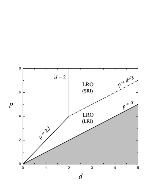
Figure 1: Regions of the ($p-d$)-plane where long-range order (LRO) takes place for a $d$-dimensional spin-$S$ Heisenberg FM model with interactions decaying as $r^{-p}$. The dashed line separates the domains where long-range interaction (LRI)- and short-range interaction (SRI)- regimes occur. The dark region corresponds to nonextensive thermodynamics not considered through this paper.

We can conclude that our low-temperature results suggest that a transition to a FM phase at a finite temperature occurs in the regions of the ($p-d$)-plane where LRO takes place. In the remaining domains a different scenario happens with absence of a phase transition. These predictions agree with the recent extensions [20] of the well known Mermin theorem [33] to spin models with LRI’s of the type here considered.

Other low-temperature thermodynamic properties follow from the general exact expressions (4.14) and (4.1). Within our approximations, the correlation functions in these equations can be expressed in terms of the transverse SD and hence the reduced internal energy $\bar{u}=u/JS^{2}$ and free energy $\overline{f}=f/JS^{2}$ per spin assume the forms

$$\bar{u}=-\bar{h}\sigma-\bar{T}\sigma\int_{1BZ}{{\frac{{d^{d}k}}{{(2\pi)^{d}}}}}{\frac{{\gamma(\vec{k})}}{{\bar{\omega}_{\vec{k}}}}}-{\frac{{1}}{{2}}\gamma(0)}\sigma^{2},$$ (4.76)

and

$$\bar{f}=\bar{f}_{0}-\bar{T}\int_{1BZ}{{\frac{{d^{d}k}}{{(2\pi)^{d}}}}}\gamma(\vec{k})\left({\int_{0}^{J}{dJ^{\prime}{\frac{{\sigma(J^{\prime})}}{{\bar{\omega}_{\vec{k}}(J^{\prime})}}}}}\right)-{\frac{1}{2}}\gamma(0)\int_{0}^{J}{dJ^{\prime}\sigma^{2}(J^{\prime})}.$$ (4.77)

In particular, in the low-temperature limit, we find

$$\bar{u}\simeq\bar{T}-\bar{h}-{\frac{1}{2}}\gamma(0)+O(\bar{T}^{2}g(\bar{h})),$$ (4.78)

where the explicit expression of the term $O(\bar{T}^{2}g(\bar{h}))$ can be obtained from Eqs. (4.62), (4.63) and (4.76) in a straightforward way. A similar low-$T$ expression can be easily obtained for $\bar{f}$. From the result (4.78), the reduced specific heat at constant magnetic field $\bar{C}_{\bar{h}}=(\partial\bar{u}/\partial\bar{T})_{\bar{h}}=C_{h}/S$ is given by

$$\bar{C}_{\bar{h}}\simeq 1+O(\bar{T}^{2}g(\bar{h})),$$ (4.79)

as expected for a classical spin model [38]. We now focus on the case $d=1$ with $p>1$ for which explicit analytical results can be obtained [24] allowing a comparison with recent MC simulations and transfer-matrix predictions. In this case, in the thermodynamic limit $N\rightarrow\infty$, we use the transformation $\sum\limits_{k}{(...)/N}\rightarrow\int_{0}^{2\pi}{dk}(...)/{2\pi}=\int_{0}^{\pi}{dk}(...)/{\pi}$ (due to the symmetry of the problem) and, for small $k$ [29, 30, 31]

$$\Omega^{(p)}(k)=\sum\limits_{n=1}^{\infty}{{\frac{{1-\cos(kn)}}{{n^{p}}}}}\simeq\left\{\begin{array}[]{lcl}\displaystyle{{\frac{1}{2}}\eta(p)k^{p-1}}&,&1<p<3\\ \\ \displaystyle{{\frac{1}{2}}k^{2}\ln\left({{\frac{1}{k}}}\right)}&,&p=3\\ \\ \displaystyle{{\frac{1}{2}}\zeta(p-2)k^{2}}&,&p>3,\end{array}\right.$$ (4.80)

where $\eta(p)=\pi\Gamma^{-1}\left(p\right){/\sin[\pi(p-2)]}$ and $\zeta(z)$ is the Riemann’s zeta function. In particular, for $p=2$, we get the exact results [39]

$$\Omega^{(2)}(k)={\frac{\pi}{2}}k-{\frac{k^{2}}{4}},\quad\quad 0\leq k\leq 2\pi\quad.$$ (4.81)

With the low-$k$ expansions (4.80), for the reduced magnetization per spin $\sigma$, we have the low-temperature representation (see Eq. (4.67))

$$\sigma(\bar{T},\bar{h}) \approx 1-\bar{T}\int_{0}^{\pi}{{\frac{{dk}}{\pi}}{\frac{1}{{\bar{h}+\Omega^{(p)}(k)}}}}$$ (4.87)

$$\approx 1-\bar{T}\left\{\begin{array}[]{lcl}\displaystyle{\overline{{h}}^{{}^{-2}}{}_{2}F_{1}\left({1,{\frac{1}{{p-1}}},{\frac{p}{{p-1}}};-{\frac{{\pi^{p-1}}}{2}}{\frac{{\eta(p)}}{{\bar{h}}}}}\right)}&,&1<p<3\\ \\ \displaystyle{\int_{0}^{\pi}{{\frac{{dk}}{\pi}}\left[{\bar{h}+{\frac{1}{2}}k^{2}\ln\left({{\frac{1}{k}}}\right)}\right]^{-1}}}&,&p=3\\ \\ \displaystyle{{\frac{2}{{\pi\zeta(p-2)}}}\sqrt{{\frac{\zeta{(p-2)}}{{2\bar{h}}}}}\arctan\left({\pi\sqrt{{\frac{\zeta{(p-2)}}{{2\bar{h}}}}}}\right)}&,&p>3,\end{array}\right.$$

where the hypergeometric function, when $\bar{h}\rightarrow 0$ behaves as

$$\overline{{h}}^{{}^{-2}}{}_{2}F_{1}\left({1,{\frac{1}{{p-1}}},{\frac{p}{{p-1}}};-{\frac{{\pi^{p-1}\eta(p)}}{{2\bar{h}}}}}\right)\approx$$ (4.94)

$$\approx \left\{\begin{array}[]{lcl}\displaystyle{{\frac{{\eta(p)\pi^{p-2}}}{{2(2-p)}}}+O(\bar{h})}&,&1<p<2\\ \\ \displaystyle{{\frac{2}{{\pi^{2}}}}\ln\left[{1+{\frac{{\pi^{2}}}{{2h}}}}\right]}&,&p=2\\ \\ \displaystyle{{\frac{2}{{\eta(p)(p-1)}}}\Gamma\left({{\frac{1}{{p-1}}}}\right)\Gamma\left({{\frac{{p-2}}{{p-1}}}}\right)\left({{\frac{{2\bar{h}}}{{\eta(p)}}}}\right)^{{\frac{{2-p}}{{p-1}}}}}&,&2<p<3.\end{array}\right.$$

According to Eqs. (4.87)-(4.94), if we write, as before, $\sigma=1-\bar{T}a(\bar{h})$, the nearly saturation condition imposes that $\bar{T}a(\bar{h})\ll 1$. For instance, with $p>3$, this condition is expressed by $\bar{T}/\sqrt{\bar{h}}\ll 1$ and hence the natural expansion parameter is $\bar{T}/\sqrt{\bar{h}}$. Of course, more accurate estimates of the integral in Eq. (4.87) can be performed including higher-order terms in the low-$k$ expansions (4.80). A check of the reliability of the estimates (4.87) can be obtained by calculating the reduced magnetization per spin to the first order in $\bar{T}$ with $p=2$ when $\Omega^{(2)}(k)$ has the exact expression (4.81). In this case, for $\bar{h}>0$, we have

$$\sigma(\bar{T},\bar{h})\simeq 1-{\frac{{\bar{T}}}{{\pi\sqrt{{\frac{{\pi^{2}}}{4}}+\bar{h}}}}}\ln\left[{{\frac{{\sqrt{{\frac{{\pi^{2}}}{4}}+\bar{h}}+{\frac{\pi}{2}}}}{{\sqrt{{\frac{{\pi^{2}}}{4}}+\bar{h}}-{\frac{\pi}{2}}}}}}\right].$$ (4.95)

For small $\bar{h}$, this reduces to

$$\sigma(\bar{T},\bar{h})\simeq 1-{\frac{{\ 2}}{\pi^{2}}}\bar{T}\ln\left[1+{\frac{\pi^{2}}{2\bar{h}}}\right],$$ (4.96)

which is just the result obtained from the hypergeometric function representation in Eq. (4.87) with $p=2$ and $\eta(2)=\pi$ assuming the low-$k$ expression $\Omega^{(2)}(k)\approx{\frac{\pi}{2}}k$ (see Eqs. 4.80) and (4.94)). Eq. (4.95) (or (4.96)) shows that the near saturation condition for $\bar{h}\rightarrow 0$ is satisfied only if $\bar{T}\ln(1/\bar{h})\ll 1$. It is worth noting that, consistently with the previous results for general $d$ (see Fig. 1), from Eq. (4.87), provided that, for small values of $\bar{h}$ (for finite $\bar{h}$ no problem occurs), the $\bar{T}$-expansion preserves its physical meaning, the following low-$\bar{T}$ features arise:

(i) for $1<p<2$, LRO occurs with a spontaneous magnetization

$$\sigma_{0}(\bar{T})=1-{\frac{{2\pi^{1-p}}}{{(2-p)\eta(p)}}}\bar{T}+O(\bar{T}^{2});$$ (4.97)

(ii) for $p\geq 2$ and $\bar{h}\rightarrow 0$, the coefficients in the $\bar{T}$ expansions in Eqs. (4.87)-(4.96) diverge and no LRO takes place at finite temperature.

From the previous equations one can immediately obtain also the reduced susceptibility. In particular, for the simplest case $p=2$ we get, exactly

$$\bar{\chi}={\frac{{\bar{T}}}{{2\pi\left({{\frac{{\pi^{2}}}{4}}+\bar{h}}\right)}}}\left\{{{\frac{\pi}{{\bar{h}}}}+{\frac{1}{\sqrt{{\frac{{\pi^{2}}}{4}}+\bar{h}}}}\ln\left[{{\frac{{\sqrt{{\frac{{\pi^{2}}}{4}}+\bar{h}}+{\frac{\pi}{2}}}}{{\sqrt{{\frac{{\pi^{2}}}{4}}+\bar{h}}-{\frac{\pi}{2}}}}}}\right]}\right\}+O(\bar{T}^{2}).$$ (4.98)

Besides, the internal and free energies per spin, and hence other thermodynamic quantities, can be obtained from Eqs. (4.76) and (4.77). In particular, for reduced internal energy per spin, we find (with $\gamma(0)=\zeta(p)$)

$$\bar{u}=\bar{T}-\bar{h}-{\frac{1}{2}}\zeta(p)+O(\bar{T}^{2}g(\bar{h}))$$ (4.99)

and hence $\bar{C}_{\bar{h}}=1+O(\bar{T}^{2}g(\bar{h}))$ as for a generic $d$.

Consistently with the previous results and exact theorems for the $d$-dimensional spin model, our analytical near saturation calculations for the classical long-range Heisenberg FM chain with $1<p<2$ predict, in a transparent way, a transition to a FM phase at finite temperature (see Fig. 1). For $p\geq 2$, a thermodynamic scenario at finite temperature, similar to that for SRI’s [14], takes place with absence of a phase transition.

Additional information about the excitation dispersion relation and thermodynamic properties for the FM chain, within nearly saturated regimes beyond the linear expansion in $\bar{T}a(\bar{h})\ll 1$, can be obtained solving numerically the full set of self-consistent Eqs. (4.58)-(4.60) with respect to $\bar{\omega}_{k}$ and $\sigma$ for $d=1$ [24]. We present here the most relevant results including comparisons with predictions obtained by means of different (and in a some sense, exact) methods. As we will see, all the numerical results confirm the previous scenario based on the estimates involving low-temperature expansions (for appropriate values of $\bar{h}$) and the dominant contributions to the dispersion relation as $k\rightarrow 0$. In Fig. 2, the reduced dispersion relation $\bar{\omega}_{k}$ is plotted as a function of $k$ in the interval $0\leq k\leq\pi$ for $\bar{T}=0$ (Fig. 2(a)) and $\bar{T}=0.5$ (Fig. 2(b)) at $\bar{h}=0.5$ with selected values of the interaction exponent $p$. The reduced magnetization $\sigma$ and susceptibility $\bar{\chi}$ in terms of $\bar{T}$ at a fixed value of $\bar{h}$ with some values of $p$ are shown in Fig. 3(a,b) where, as a comparison, transfer-matrix results for the Heisenberg FM chain with SRI’s ($p=\infty$) [14, 40] are also presented. The plots of the reduced magnetization per spin $\sigma$ as a function of $\bar{h}$ for some values of $\bar{T}$ with $p=1.5$ in Fig. 4(a) and for different values of $p$ with $\bar{T}=0.1$ in Fig. 4(b) are particularly meaningful.

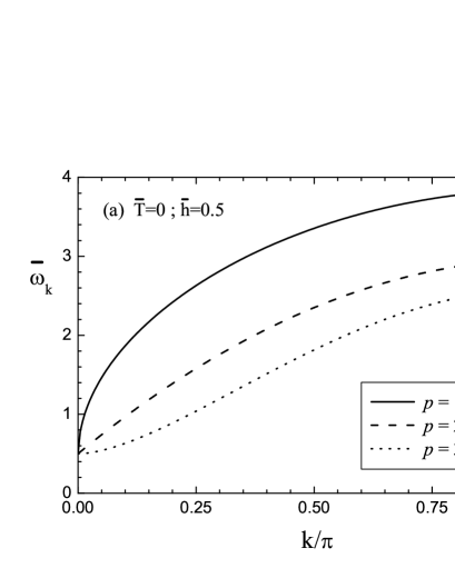
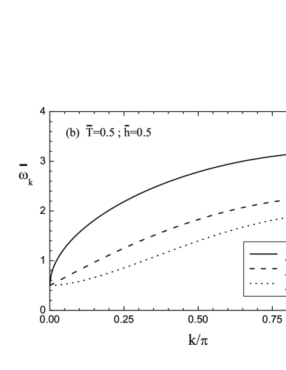
Figure 2: Dispersion relation $\overline{\omega}_{k}$ of an Heisenberg FM chain as a function of $k$ in the interval $\left[0,\pi\right]$ for reduced magnetic field $\overline{h}=0.5$ and temperature $\overline{T}=0$ (a) and $\overline{T}=0.5$ (b) with different values of the decaying parameter $p$.

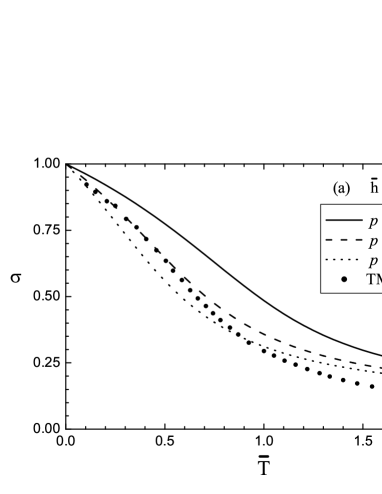
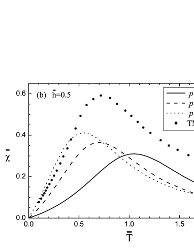
Figure 3: Temperature dependence of the reduced magnetization $\sigma$ (a) and susceptibility $\overline{\chi}$ (b) of an Heisenberg FM chain for $\overline{h}=0.5$ and different values of $p$. The dots represent the transfer-matrix (TM) results for SRI’s ($p=\infty$).

Figure 4: Reduced magnetization $\sigma$ of an Heisenberg FM chain as a function of $\overline{h}$ for (a) $p=1.5$ and different values of $\overline{T}$ and (b) $\overline{T}=0.1$ and different values of $p$.

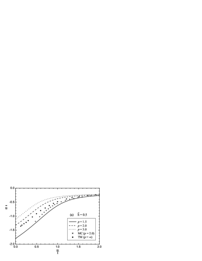
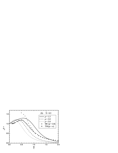
Figure 5: Temperature dependence of the reduced (a) internal energy $\overline{u}$ and (b) specific heat $\overline{C}_{\overline{h}}$ of an Heisenberg FM chain for $\overline{h}=0.5$ and different values of $p$. The stars represent Monte Carlo (MC) results for $p=2$ and the dots TM predictions for SRI’s ($p=\infty$).

They show clearly our previous analytical finding that, for $1<p<2$, a FM phase occurs at finite temperature. Of course, at this stage, our ME’s do not allow to study regimes with $\sigma\rightarrow 0$ as $\bar{h}\rightarrow 0$ and hence to find the transition point to the FM phase where $1<p<2$. Information about this transition and the related critical properties will be given in the next subsection. The reduced internal energy $\bar{u}$ and the specific heat $\bar{C}_{\bar{h}}$, evaluated from the solutions of the $(d=1)$-ME’s (4.58)-(4.60), are also plotted in Figs. 5(a) and 5(b) as functions of $\bar{T}$ for different values of $p$. In both these figures, as a further comparison, we have also reported the transfer-matrix results for the short-range chain [14, 40] and MC simulations recently obtained [21] for a classical long-range FM Heisenberg chain with $p=2$. Finally, in Fig.6, we present the behavior of the transverse correlation length $\xi_{\perp}$ as a function of $\bar{T}$ for $\bar{h}=0.5$ and different values of $p$. Notice that a substantial difference clearly occurs for $1<p<2$ and $p\geq 2$, respectively. Again, in the same figure, we have plotted also transfer-matrix results for a FM chain with SRI’s [14, 40].

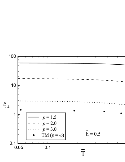
Figure 6: Temperature dependence of the transverse correlation length $\xi_{\perp}$ of an Heisenberg FM chain for $\overline{h}=0.5$ and different values of $p$ (with logarithmic scales). The dots represent TM results for SRI’s ($p=\infty$).

4.4.2 Thermodynamic Regimes with Near-zero Magnetization

As discussed in Subsec. 4.3.1, Eq. (4.42) for the dispersion relation, or the first expression for $R(\vec{k})$ in Eq (4.60), is inadequate to obtain suitable results for thermodynamics regimes with near-zero magnetization ($\sigma\rightarrow 0$). However, this case can be successfully explored using the self-consistent ME’s (4.58)-(4.59) with the simple modification for $R(\vec{k})$ given in Eq. (4.60) when $\sigma\rightarrow 0$. Below, we show indeed that the modified ME’s can be properly used for an estimate of the main critical properties of our classical spin model, when it starts to exhibit LRO, and of the low-temperature paramagnetic susceptibility in the remaining regions of the ($p-d$)-plane when no LRO exists.

A. Transition temperature and critical properties

In the limit $\overline{h}\rightarrow 0$ with $\sigma\geq 0$, the system of Eqs. (4.58)-(4.59), with $R(\vec{k})$ appropriate to include the case $\sigma\rightarrow 0$, assumes the form [27]

$$\bar{\omega}_{\vec{k}} = \sigma\Omega^{(p)}({\vec{k}})R({\vec{k}})\ ,$$ (4.100)

$$R({\vec{k}}) = =1+{\frac{\overline{T}}{\Omega^{(p)}({\vec{k}})}}\int_{1BZ}{\frac{d^{d}k^{\prime}}{(2\pi)^{d}}}{\frac{\Omega^{(p)}({\vec{k}}-{\vec{k}}^{\prime})-\Omega^{(p)}({\vec{k}}^{\prime})}{\Omega^{(p)}({\vec{k}}^{\prime})R({\vec{k}}^{\prime})}}\ ,$$ (4.101)

$$\sigma^{2} = {\frac{1-3{\overline{T}}Q({\overline{T}})}{{1-{\overline{T}}Q({\overline{T}})}}}\ ,$$ (4.102)

where

$$Q({\overline{T}})=\int_{1BZ}{\frac{d^{d}k}{(2\pi)^{d}}}{\frac{1}{\Omega^{(p)}({\vec{k}})R({\vec{k}})}}\ .$$ (4.103)

From Eq. (4.102) we can immediately obtain an equation which determines the critical temperature $T_{c}$ (when it exists). Indeed, the reduced critical temperature ${\overline{T}}_{c}$ (with $T_{c}=JS^{2}{\overline{T}}_{c}$) can be obtained setting $\sigma({\overline{T}}_{c})=0$. This yields the equation

$$1-3{\overline{T}}_{c}Q({\overline{T}}_{c})=0.$$ (4.104)

It is not simple to solve exactly this equation and one must resort again to numerical calculations. However, it is instructive to get an explicit estimate of ${\overline{T}}_{c}$ by calculating the integrals in Eqs. (4.100)-(4.103) taking for $\Omega^{(p)}({\vec{k}})$ the dominant contribution as ${\vec{k}}\rightarrow 0$. Then, solving by iteration our self-consistent ME’s, to first level of iteration we have

$$Q({\overline{T}})\simeq\frac{\mathcal{F}_{1}^{(p)}(0)}{1+\overline{T}\mathcal{F}_{1}^{(p)}(0)},$$ (4.105)

and

$$\bar{\omega}_{\vec{k}}\simeq\Omega^{(p)}({\vec{k}})\sigma({\overline{T}})\left[1+\overline{T}\mathcal{F}_{1}^{(p)}(0)\right],$$ (4.106)

where $\mathcal{F}_{1}^{(p)}(0)$ and $\sigma({\overline{T}})$ are given by Eqs. (4.64) (for $\overline{h}=0$) and (4.102), respectively. With $Q({\overline{T}})$ explicitly known, Eq. (4.104) yields for ${\overline{T}}_{c}={\overline{T}}_{c}(p,d)$

$${\overline{T}}_{c}={\frac{1}{2\mathcal{F}_{1}^{(p)}(0)}}\ .$$ (4.107)

From this simple expression, one immediately sees that a critical temperature exists only when $\mathcal{F}_{1}^{(p)}(0)$ is finite and hence in the regions of the $(p-d)$- plane where LRO occurs. Here we explicitly consider the one-dimensional case for $1<p<2$ and the two-dimensional one for $2<p<4$ for which a comparison with recent alternative analytical and MC results can be performed.

For $d=1$ and $1<p<2$ one finds [24]

$${\overline{T}}_{c}(d=1)={\frac{(2-p)\eta(p)}{4\pi^{1-p}}}\ .$$ (4.108)

In particular, for $p\rightarrow 2^{-}$, Eq. (4.108) yields $T_{c}=JS^{2}{\overline{T}}_{c}\approx\pi^{2}JS^{2}(2-p)/4$ to be compared with $T_{c}\approx\pi^{2}JS(S+1)(2-p)/3$, obtained in Ref. [31] for the quantum case by means of the EMM, and with $T_{c}\propto JS^{2}(2-p)$ derived by Kosterlitz [36] for the classical chain using a perturbative renormalization group approach.

For the case $d=2$ with $2<p<4$, the coefficients of interest in the low-$k$ expansions (4.66) for $\Omega^{(p)}({\vec{k}})$ are given by [31]

$$\left\{\begin{array}[]{l}\displaystyle{A_{2}=2^{2-p}\pi^{2}\Gamma^{-2}(p)/\sin[\pi(p-2)/2]}\\ \\ \displaystyle{B_{2}=2^{p-2}\zeta\left({\frac{p-2}{2}}\right)\left[\zeta\left({\frac{2-p}{2}},{\frac{1}{4}}\right)-\zeta\left({\frac{2-p}{2}},{\frac{3}{4}}\right)\right]}\end{array}\right.,~{}2<p<4,$$ (4.109)

where $\zeta(z,a)=\sum_{n=0}^{\infty}(n+a)^{-z}$ is the generalized Riemann zeta function and $\zeta(z)\equiv\zeta(z,0)$ is the ordinary Riemann zeta function. Then, in Eq. (4.107), we have

$$\left.\mathcal{F}_{1}^{(p)}(0)\right|_{d=2}\simeq\frac{\Lambda^{2-p}}{{4-p}}\frac{\Gamma^{2}(p)}{2^{1-p}\pi^{2}}\sin\left[\pi(p-2)/2\right]\mathcal{\,,}$$ (4.110)

and hence

$${\overline{T}}_{c}(d=2)={\frac{(4-p)\pi^{2}\Lambda^{p-2}}{2^{p}\Gamma^{2}(p)\sin\left[\pi(p-2)/2\right]}}\ .$$ (4.111)

In Fig. 7 the critical temperature of $(S={\frac{1}{2}})$-models, for $d=1$ (Fig. 7(a)) and $d=2$ (Fig. 7(b)), is plotted as a function of $p$ and compared with the corresponding results recently obtained, for the long-range quantum Heisenberg model by means of the EMM, within the Tyablikov decoupling, for both cases $d=1$ and $d=2$ [31], the modified spin-wave theory [29] and MC simulations [32], for $d=2$. Our results appear to be consistent with those obtained for the quantum counterpart if we keep in mind that the apparent discrepancy is related to the known feature that a quantum spin-$S$ model can be reasonably approximated by a classical one only in the large-$S$ limit [41].

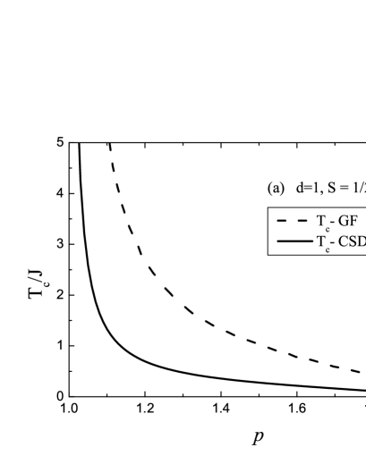
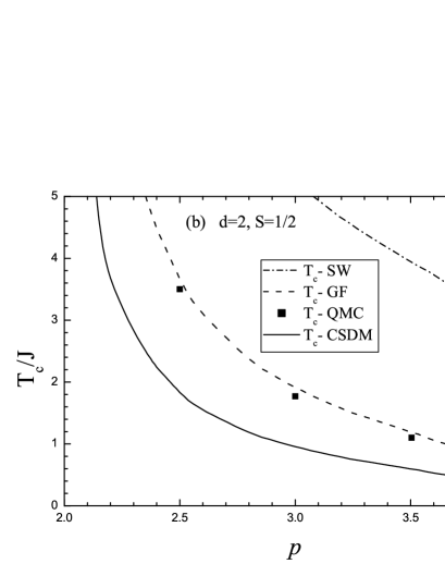
Figure 7: Critical temperature as a function of the decaying parameter $p$ for a one-dimensional (a) and two-dimensional (b) spin-$1/2$ Heisenberg ferromagnet. The dashed lines refer to the Green function (GF) method and to the modified spin-wave (SW) theory results, respectively. The dots represent MC predictions.

From Eq. (4.102), we can easily obtain the behavior of the magnetization per spin $m(T)=\sigma({\overline{T}})S$, with ${\overline{T}}=T/JS^{2}$. For all values of $p$ and $d$ for which a phase transition occurs, we get

$$m(T)\sim\left({\frac{T-T_{c}}{T_{c}}}\right)^{1/2}\ ,$$ (4.112)

implying $\beta=1/2$ for the magnetization critical exponent.

The calculations are more delicate to obtain the near criticality behavior of the paramagnetic susceptibility defined as $\chi=J{\overline{\chi}}=J(\sigma/\overline{h})$ in the limit $\overline{h}\rightarrow 0$ with $\sigma\rightarrow 0$. In this case, the set of Eqs. (4.58)-(4.59), with the appropriate expression for $R({\vec{k}})$ in Eq. (4.60), reduces to

$$1 = 3{\overline{\chi}}{\overline{T}}\int_{1BZ}{\frac{d^{d}k}{(2\pi)^{d}}}{\frac{1}{1+{\overline{\chi}}P({\vec{k}})}}\ ,$$ (4.113)

$$P({\vec{k}}) = \Omega^{(p)}({\vec{k}})+{\overline{\chi}}{\overline{T}}\int_{1BZ}{\frac{d^{d}k^{\prime}}{(2\pi)^{d}}}{\frac{\Omega^{(p)}({\vec{k}}-{\vec{k}}^{\prime})-\Omega^{(p)}({\vec{k}}^{\prime})}{1+{\overline{\chi}}P({\vec{k}}^{\prime})}}\ ,$$ (4.114)

with $P(\vec{k})=\Omega^{(p)}({\vec{k}})R({\vec{k}})$. Of course, these equations can only be solved numerically. However, an estimate of $\chi(T)$ as $T\rightarrow T_{c}^{+}$, can be obtained assuming, as usual, the low-$k$ behaviors (4.66) for $\Omega^{(p)}(\vec{k})$. Then, a solution of Eqs. (4.113) and (4.114), with ${\overline{\chi}}({\overline{T}})\rightarrow\infty$ as ${\overline{T}}\rightarrow{\overline{T}}_{c}^{+}$, is found to be

$$\chi=J{\overline{\chi}}\sim\left({\frac{T-T_{c}}{T_{c}}}\right)^{-\gamma(p,d)}\ ,$$ (4.115)

where the $(p,d)$-dependent susceptibility critical exponent $\gamma(p,d)$ is given in Table I for the different regions of the $(p-d)$-plane where LRO exists, together with other critical exponents to be obtained below.

Table I

Critical exponent $\frac{3}{2}d<p<\left\{\begin{array}[]{lll}2d&,&d\leq 2\\ d+2&,&d>2\end{array}\right.$ $p=\frac{3}{2},\quad d\leq 4$ $d<p<\left\{\begin{array}[]{lll}\frac{3}{2}d&,&d<4\\ d+2&,&d>4\end{array}\right.$ $2<d<4$ $p\geq d+2$ $d=4$ $d>4$ $\beta(p,d)$ $1/2$ $1/2$ $1/2$ $1/2$ $1/2$ $1/2$ $\gamma(p,d)$ $\frac{p-d}{2d-p}$ $1_{\ln}$ $1$ $\frac{2}{d-2}$ $1_{\ln}$ $1$ $\delta(p,d)$ $\frac{p}{2d-p}$ $3_{\ln}$ $3$ $\frac{d+2}{d-2}$ $3_{\ln}$ $3$ $\alpha(p,d)$ $\frac{3d-2p}{2d-p}$ $0_{\ln}$ $0$ $\frac{d-4}{d-2}$ $0_{\ln}$ $0$

Table 1: Main ($p,d$)-dependent critical exponents in different domains of the ($p-d$)-plane where LRO exists. The double vertical lines separate the regions where LRI’s are active and SRI regime occurs. The symbol $x_{ln}$ denotes the main ($T-T_{c}$)- or $h$- dependence with a logarithmic correction (for instance, $\chi(T)\sim(T-T_{c})^{-1}\ln\left[1/(T-T_{c})\right]$, $m(h)\sim h^{1/3}\left|\ln h\right|^{1/3}$, etc.)

We now determine the behavior of the magnetization per spin $m$ along the critical isotherm as $h\rightarrow 0$. It is easy to see that, from the basic ME’s (4.58)-(4.60), the equation of the critical isotherm for small $\overline{h}$ and $\sigma$ assumes the form

$$1-{\frac{2}{3}}\sigma^{2}-3{\overline{T}}_{c}Q_{c}\left({\sigma/\overline{h}}\right)=0\ ,$$ (4.116)

where

$$Q_{c}\left({\sigma/\overline{h}}\right)=\left({\sigma/\overline{h}}\right)\int_{1BZ}{\frac{d^{d}k}{(2\pi)^{d}}}{\frac{1}{1+{\frac{\sigma}{\overline{h}}}P_{c}({\vec{k}})}}\ ,$$ (4.117)

and $P_{c}({\vec{k}})$ is obtained from Eq. (4.114) with $\overline{\chi}$ replaced by $\sigma/\overline{h}$ and ${\overline{T}}={\overline{T}}_{c}$. Eqs. (4.116) and (4.117) can be solved numerically but a suitable estimate of $\sigma$ as ${\overline{h}}\rightarrow 0$ can be easily obtained working again in terms of the dominant contribution of $\Omega^{(p)}({\vec{k}})$ as ${\vec{k}}\rightarrow 0$. Then, we get

$$m=\sigma S\sim h^{1/\delta(p,d)},$$ (4.118)

where the expressions of the critical exponent $\delta(p,d)$ in the different domains of the $(p-d)$-plane are given in Table I.

Finally, we wish to calculate the critical exponent $\alpha(p,d)$ of the specific heat in zero magnetic field as $T\rightarrow T_{c}^{+}$ for values of $p$ and $d$ such that a transition to the FM phase takes place. It is worth noting that, for this purpose, one cannot use the expression (4.76) for the reduced internal energy per spin. Indeed, it has a physical meaning only in the thermodynamic regimes where the decoupling $\langle S_{{\vec{k}}}^{z}S_{-{\vec{k}}}^{z}\rangle\simeq\langle S_{{\vec{k}}}^{z}\rangle\langle S_{-{\vec{k}}}^{z}\rangle$ can be used. A reliable calculation can be rather performed using the general expression (4.14) with the decoupling procedure (4.3.1) appropriate near the critical point, where $\sigma\rightarrow 0$, which takes into account the effects of the longitudinal spin correlations. From this expression, one can easily show that the reduced internal energy per spin near criticality assumes the form

$${\overline{u}}\simeq-{\overline{h}}\sigma-{\frac{1}{2}}\gamma(0)\sigma^{2}-{\frac{1}{2}}{\overline{T}}\sigma(1+\sigma^{2})\int_{1BZ}{\frac{d^{d}k}{(2\pi)^{d}}}{\frac{\gamma({\vec{k}})}{{\overline{\omega}}_{{\vec{k}}}}}\ ,$$ (4.119)

where now ${\overline{\omega}}_{{\vec{k}}}$ is given by Eq. (4.58) with the appropriate $R({\vec{k}})$ in Eq. (4.60). With Eq. (4.119) we have all the ingredients to calculate the zero-field specific heat near criticality. Indeed, working at ${\overline{h}}\rightarrow 0$ and $\sigma\rightarrow 0$ with $\sigma/{\overline{h}}={\overline{\chi}}({\overline{T}})$ as ${\overline{T}}\rightarrow{\overline{T}}_{c}^{+}$ and taking into account Eq. (4.113) with $P({\vec{k}})$ evaluated as ${\vec{k}}\rightarrow 0$, Eq. (4.119) can be conveniently expressed, in terms of ${\overline{T}}$, $\overline{\chi}$ and $\overline{h}$, as

$${\overline{u}}\simeq{\frac{1}{2}}{\overline{T}}-{\overline{h}}^{2}{\overline{\chi}}-{\frac{1}{2}}\gamma(0){\overline{h}}^{2}{\overline{\chi}}^{2}-{\frac{1}{6}}(1+\gamma(0){\overline{\chi}}){\overline{\chi}}^{-1}\ .$$ (4.120)

Then, for the reduced zero-field specific heat ${\overline{C}}_{\overline{h}=0}({\overline{T}})=C_{h=0}(T)/S$, we have

$$C_{\overline{h}=0}({\overline{T}})=\left({\frac{\partial\overline{u}}{\partial{\overline{T}}}}\right)_{\overline{h}=0}\simeq{\frac{1}{2}}+{\frac{1}{6}}\overline{\chi}^{-2}{\frac{\partial\overline{\chi}}{\partial{\overline{T}}}}\ ,\qquad({\overline{T}}\rightarrow{\overline{T}}_{c}^{+}).$$ (4.121)

From this expression one can immediately determine the specific heat critical exponent $\alpha(p,d)$. Indeed, with $\overline{\chi}({\overline{T}})\sim A({\overline{T}}-{\overline{T}}_{c})^{-\gamma}$ or $\overline{\chi}({\overline{T}})\sim A({\overline{T}}-{\overline{T}}_{c})^{-1}\ln\left[{\frac{1}{({\overline{T}}-{\overline{T}}_{c})}}\right]$ (see Table I), Eq. (4.121) yields

$${\overline{C}}_{\overline{h}=0}({\overline{T}})\simeq\left\{\begin{array}[]{lcl}\displaystyle{{\frac{1}{2}}-{\frac{1}{6}}\gamma(p,d)A^{2}({\overline{T}}-{\overline{T}}_{c})^{-\alpha(p,d)}}&,&\alpha(p,d)=1-\gamma(p,d)<0,\\ \\ \displaystyle{{\frac{1}{2}}-{\frac{1}{6}}A^{2}({\overline{T}}-{\overline{T}}_{c})^{0}\ln^{-1}\left[{\frac{1}{{\overline{T}}-{\overline{T}}_{c}}}\right]}&,&\alpha=O_{\ln}\ .\end{array}\right.$$ (4.122)

From these relations and the exponent $\gamma(p,d)$ found before, one can immediately obtain the explicit expression for $\alpha(p,d)$. The different values of $\alpha(p,d)$ varying $p$ and $d$ are also given in Table I. Other critical exponents can be obtained using the known scaling laws.

The data collected in Table I show clearly some features which signal the degree of efficiency of the approximations made to lowest order in the CSDM. First, the critical exponents coincide with those for the classical spherical model. Besides, within the region denoted with LRO (SRI) in Fig. 1, the critical exponents are exactly the same of those for the short-range Heisenberg model. This suggests that improving systematically the one-pole approximation for $\Lambda_{\vec{k}}(\omega)$ within the spirit of the SDM may produce better results beyond the mean-field approximation.

As a conclusion we note that for $d=1$ with $1<p<2$, when the LRI’s are active, the explicit expressions of the coefficients in the power laws (4.112), (4.115), (4.118) and (4.122), as functions of $p$, can be found in Ref. [24].

B. Low-temperature paramagnetic susceptibility in absence of LRO

For obtaining the low-temperature zero-field susceptibility in absence of LRO, namely for $p\geq 2d$ and $d\leq 2$ in Fig. 1, one can use again Eqs. (4.113)-(4.114) but bearing in mind that now $T_{c}=0$. Then, with the same procedure used before for determining the near critical behavior of the paramagnetic susceptibility as $T\rightarrow T_{c}^{+}$ when LRO occurs, we easily find, for reduced susceptibility as $T\rightarrow 0$,

$$\overline{\chi}({\overline{T}})\sim\left\{\begin{array}[]{lcl}\exp[A_{d}\Lambda^{d}/3{\overline{T}}]&,&p=2d\\ {\overline{T}}^{-{\frac{p-d}{p-2d}}}&,&2d<p<2+d\\ {\overline{T}}^{-{\frac{2}{2-d}}}\left(\ln\left[{\frac{1}{{\overline{T}}}}\right]\right)^{\frac{d}{2-d}}&,&p=2+d\\ {\overline{T}}^{-{\frac{2}{2-d}}}&,&p>2+d\ .\end{array}\right.$$ (4.123)

As usual, for $d=1$, all the coefficients can be explicitly calculated and Eq. (4.123) becomes

$$\overline{\chi}({\overline{T}})\simeq\left\{\begin{array}[]{lcl}{\frac{3}{4\pi^{2}}}\exp\left[2\pi^{2}/9{\overline{T}}\right]&,&p=2\\ \left[\left({\frac{4}{3}}\right)^{\frac{1}{(p-1)}}{\frac{1}{3A(p)}}\right]^{{\frac{(p-1)}{(p-2)}}}{\overline{T}}^{-{\frac{p-1}{p-2}}}&,&2<p<3\\ \frac{16}{27}{\overline{T}}^{-{2}}\ln\left[{\frac{1}{{\overline{T}}}}\right]&,&p=3\\ \frac{8}{27}\zeta(p-2){\overline{T}}^{-{2}}&,&p>3\ ,\end{array}\right.$$ (4.124)

where

$$A(p)={\frac{2\left[2({\frac{3}{2}})^{\frac{2p-3}{p-1}}-1\right]}{9(p-1)^{3}}}\left[\sin\left({\frac{\pi}{p-1}}\right)\right]^{-1}\left({\frac{1}{2}}\eta(p)\right)^{-\frac{1}{p-1}}\ .$$ (4.125)

The previous results for $d=1$ appear consistent with the ones obtained in Refs. [29, 31] for the corresponding quantum Heisenberg chain. It is worth noting an important aspect of the result in Eq. (4.123) for $p=2d$ and hence in Eq. (4.124) for $p=2$. This finding for reduced susceptibility, although consistent with the one obtained by means of the modified spin-wave theory [29] and the EMM for the two-time GF’s [31] for quantum model, does not reproduce the well known exact Haldane result for $d=1$ [42] which contains a factor proportional to ${\overline{T}}^{-1/2}$. So, we are induced to argue that one must expect a $d$-dependent power factor in ${\overline{T}}$ in Eq. (4.123) which corrects the pure low temperature exponential divergence reproducing ${\overline{T}}^{-1/2}$ for $d=1$. However, the lowest-order approximation in the CSDM, used in our calculations, has been able to capture the exponential divergence as ${\overline{T}}\rightarrow 0$ and, hopefully, one can improve systematically this result by means of higher order approximations.

4.5 Moment Equations within the two $\delta$-poles Approximation for the
Transverse Spectral Density

The next higher order approximation in the CSDM is to use the three exact ME’s (4.34)-(4.3) and to choose a two $\delta$-functions structure for the $\Lambda_{\vec{k}}(\omega)$ involving three unknown parameters (see Subsec. 3.2). A reliable possibility, suggested by quantum studies [4, 5, 7, 8, 9, 10, 11], is

$$\Lambda_{\vec{k}}(\omega)=2\pi\left\{{\lambda_{\vec{k}}^{(1)}\delta(\omega-\omega_{\vec{k}})+\lambda_{\vec{k}}^{(2)}\delta(\omega+\omega_{\vec{k}})}\right\},$$ (4.126)

so that, Eqs. (4.34)-(4.3) yield

$$\begin{array}[]{l}\lambda_{\vec{k}}^{(1)}+\lambda_{\vec{k}}^{(2)}=M_{0}(\vec{k})=2Nm,\\ \omega_{\vec{k}}(\lambda_{\vec{k}}^{(1)}-\lambda_{\vec{k}}^{(2)})=M_{1}(\vec{k}),\\ \omega_{\vec{k}}^{2}(\lambda_{\vec{k}}^{(1)}+\lambda_{\vec{k}}^{(2)})=M_{2}(\vec{k}),\end{array}$$ (4.127)

where $M_{\nu}({\vec{k}})$ $(\nu=1,2)$ denote the moments in the right-hand side of the Eqs. (4.3) and (4.3), respectively. These moments involve higher order correlation functions of the spin variables and hence, to close the set of ME’s (4.127), it is necessary to use appropriate decoupling procedures. Below we suggest some of them which can be conveniently used for higher order calculations.

4.5.1 Full Neglect of Longitudinal Spin Correlations

Using in Eqs. (4.3)-(4.3) the Tyablikov-like decoupling procedure

$$\left\langle{S_{\vec{k}}^{+}S_{\vec{q}}^{-}S_{\vec{p}}^{z}}\right\rangle\simeq\left\langle{S_{\vec{p}}^{z}}\right\rangle\left\langle{S_{\vec{k}}^{+}S_{\vec{q}}^{-}}\right\rangle$$ (4.128)

and the trivial ones $\left\langle{S_{\vec{k}}^{z}S_{\vec{q}}^{z}}\right\rangle\simeq\left\langle{S_{\vec{k}}^{z}}\right\rangle\left\langle{S_{\vec{q}}^{z}}\right\rangle$ and $\left\langle{S_{\vec{k}}^{z}S_{\vec{q}}^{z}S_{\vec{p}}^{z}}\right\rangle\simeq\left\langle{S_{\vec{k}}^{z}}\right\rangle\left\langle{S_{\vec{q}}^{z}}\right\rangle\left\langle{S_{\vec{p}}^{z}}\right\rangle$, in Eq. (4.127) we have

$$M_{1}(\vec{k}) = 2Nm\omega_{\vec{k}}^{(Ty)}+{\frac{{T}}{N}}\sum\limits_{\vec{k}^{\prime}}{\left[{J(\vec{k}^{\prime})-J(\vec{k}-\vec{k}^{\prime})}\right]{\frac{{\lambda_{\vec{k}^{\prime}}^{(1)}-\lambda_{\vec{k}^{\prime}}^{(2)}}}{{\omega_{\vec{k}^{\prime}}}}}},$$ (4.129)

$$M_{2}(\vec{k}) = 2Nm\left({\omega_{\vec{k}}^{(Ty)}}\right)^{2}+2{\omega_{\vec{k}}^{(Ty)}\frac{{T}}{N}}\sum\limits_{\vec{k}^{\prime}}{\left[{J(\vec{k}^{\prime})-J(\vec{k}-\vec{k}^{\prime})}\right]{\frac{{\lambda_{\vec{k}^{\prime}}^{(1)}-\lambda_{\vec{k}^{\prime}}^{(2)}}}{{\omega_{\vec{k}^{\prime}}}},}}$$

which close the set of ME’s (4.127). In the previous equations $\omega_{{\vec{k}}}^{(Ty)}$ is given by Eq. (4.25) and use is made of the relation (4.37) which expresses exactly the transverse spin correlation function $\left\langle{S_{\vec{k}}^{+}S_{-\vec{k}}^{-}}\right\rangle$ in terms of $\Lambda_{\vec{k}}(\omega)$. From Eqs. (4.127) and (4.129)-(4.129), we can conveniently write a set of two self-consistent integral equations for $M_{1}({\vec{k}})$ and $M_{2}({\vec{k}})$ and then determine the parameters $\omega_{\vec{k}}$ and $\lambda_{\vec{k}}^{(\nu)}$ $(\nu=1,2)$ in terms of $M_{1}({\vec{k}})$ and $M_{2}({\vec{k}})$. Indeed, by Eqs. (4.127), it is easy to show that

$${\frac{{M_{1}(\vec{k})}}{{2Nm}}}=\omega_{\vec{k}}^{(Ty)}+{\frac{{T}}{N}}\sum\limits_{\vec{k}^{\prime}}{\left[{J(\vec{k}^{\prime})-J(\vec{k}-\vec{k}^{\prime})}\right]{\frac{{M_{1}(\vec{k}^{\prime})}}{{M_{2}(\vec{k}^{\prime})}}}},$$ (4.131)

and

$${\frac{{M_{2}(\vec{k})}}{{2Nm}}}=\left({\omega_{\vec{k}}^{(Ty)}}\right)^{2}+{2\omega_{\vec{k}}^{(Ty)}\frac{{T}}{N}}\sum\limits_{\vec{k}^{\prime}}{\left[{J(\vec{k}^{\prime})-J(\vec{k}-\vec{k}^{\prime})}\right]{\frac{{M_{1}(\vec{k}^{\prime})}}{{M_{2}(\vec{k}^{\prime})}}}},$$ (4.132)

with

$$\omega_{\vec{k}}^{2}={\frac{{M_{2}(\vec{k})}}{{2Nm}}},$$ (4.133)

and

$$\lambda_{\vec{k}}^{(\nu)}=Nm+(-1)^{\nu+1}{\frac{{M_{1}(\vec{k})}}{2}}\left({{\frac{{2Nm}}{{M_{2}(\vec{k})}}}}\right)^{{\frac{1}{2}}},\quad(\nu=1,2).$$ (4.134)

Of course, when Eqs. (4.131)-(4.132) are solved and hence $M_{1}({\vec{k}})$ and $M_{2}({\vec{k}})$ are known, Eqs. (4.133)-(4.134) determine $\Lambda_{\vec{k}}(\omega)$, as given by Eq. (4.126), and all the thermodynamic properties follow from the general formulas established in Subsec. 4.1. In particular, for the dispersion relation $\omega_{\vec{k}}$ of the undamped oscillations and the magnetization per spin, we find

$$\omega_{\vec{k}}=\omega_{\vec{k}}^{(Ty)}\left\{{1+{\frac{{2}}{{\omega_{\vec{k}}^{(Ty)}}}}{\frac{T}{N}}\sum\limits_{\vec{k}^{\prime}}{\left[{J(\vec{k}^{\prime})-J(\vec{k}-\vec{k}^{\prime})}\right]{\frac{{M_{1}(\vec{k}^{\prime})}}{{M_{2}(\vec{k}^{\prime})}}}}}\right\}^{{\frac{1}{2}}}$$ (4.135)

and

$$m\simeq S-{\frac{{T}}{N}}\sum\limits_{\vec{k}}{{\frac{{M_{1}(\vec{k})}}{{M_{2}(\vec{k})}}.}}$$ (4.136)

We wish to underline that the previous results are physically meaningful only for ($T$,$h$)-values in the nearly saturated regimes where, neglecting the longitudinal spin correlations, they constitute a reasonable approximation.

Equations (4.131)-(4.136) show that it is convenient to work in terms of the single parameter

$$x(\vec{k})={\frac{{M_{1}(\vec{k})}}{{M_{2}(\vec{k})}}},$$ (4.137)

satisfying the self-consistent equation

$$x(\vec{k})={\frac{1}{{\omega_{\vec{k}}^{(Ty)}}}}{\frac{{1+{\frac{{1}}{{\omega_{\vec{k}}^{(Ty)}}}}{\frac{T}{N}}\sum\limits_{\vec{k}^{\prime}}{\left[{J(\vec{k}^{\prime})-J(\vec{k}-\vec{k}^{\prime})}\right]x(\vec{k}^{\prime})}}}{{1+{\frac{{2}}{{\omega_{\vec{k}}^{(Ty)}}}}{\frac{T}{N}}\sum\limits_{\vec{k}^{\prime}}{\left[{J(\vec{k}^{\prime})-J(\vec{k}-\vec{k}^{\prime})}\right]x(\vec{k}^{\prime})}}}}.$$ (4.138)

A full solution of this equation is of course inaccessible and one must resort to numerical calculations. However, analytical results can be obtained, as usual, by expansion in powers of $T$ with $\frac{1}{N}\sum\limits_{\vec{k}^{\prime}}{(...)\rightarrow\int_{1BZ}{d^{d}k^{\prime}(...)/}(2\pi)^{d}}$ and appropriate constraints on the values of $h$ assuring the convergency of the integrals (see discussion in Subsec. 4.4.1). Working, for instance, to first order in $T$, Eqs. (4.131), (4.132) and (4.136) yield

$$m\simeq S\left\{{1-{\frac{{T}}{{JS^{2}}}}\mathcal{F}_{1}^{(p)}(\bar{h})}\right\},$$ (4.139)

which is exactly the same result (4.63) obtained with the one $\delta$-pole ansatz for $\Lambda_{\vec{k}}(\omega)$. Then, from Eq. (4.138), one easily has

$$x(\vec{k})\simeq\omega_{0\vec{k}}^{-1}\left\{{1+{\frac{{T}}{{\omega_{0\vec{k}}S}}}\left[{\mathcal{F}_{1}^{(p)}(\bar{h})\Omega^{(p)}(\vec{k})+\mathcal{F}_{2}^{(p)}(\bar{h},\vec{k})}\right]}\right\}$$ (4.140)

where $\mathcal{F}_{\nu}^{(p)}(\bar{h},\vec{k})$ $(\nu=1,2)$ are defined by Eqs. (4.64) and (4.65) and $\omega_{0{\vec{k}}}=\omega_{\vec{k}}^{(Ty)}\left|{{}_{T=0}}\right.=JS\left({\bar{h}}+\Omega^{(p)}(\vec{k})\right)$. Of course, an estimate of the integrals $\mathcal{F}_{\nu}^{(p)}$ can be made using the expansions (4.66) for $\Omega^{(p)}(\vec{k})$ as $\vec{k}\rightarrow 0$ along the lines outlined in Subsec. 4.4.1.

Now, from Eqs. (4.131), (4.132) and (4.137), a straightforward algebra yields

$$M_{1}(\vec{k})\simeq 2NS\omega_{0\vec{k}}\left\{{1-{\frac{{T}}{{JS^{2}}}}\left[\mathcal{F}_{1}^{(p)}(\bar{h})+\frac{{JS}}{{\omega_{0\vec{k}}}}\left(\mathcal{F}{{}_{1}^{(p)}(\bar{h})\Omega^{(p)}(\vec{k})+\mathcal{F}_{2}^{(p)}(\bar{h},\vec{k})}\right)\right]}\right\},$$ (4.141)

and

$$M_{2}(\vec{k})\simeq 2NS\omega_{0\vec{k}}^{2}\left\{{1-{\frac{{T}}{{JS^{2}}}}\left[\mathcal{F}_{1}^{(p)}(\bar{h})+\frac{{JS}}{{\omega_{0\vec{k}}}}\left({\mathcal{F}_{1}^{(p)}(\bar{h})\Omega^{(p)}(\vec{k})+\mathcal{F}_{2}^{(p)}(\bar{h},\vec{k})}\right)\right]}\right\}.$$ (4.142)

Then, Eqs. (4.133) and (4.134) provide

$$\omega_{\vec{k}}\simeq\omega_{0\vec{k}}\left\{1-\frac{{T}}{{\omega_{0\vec{k}}S}}\left[\mathcal{F}{{}_{1}^{(p)}(\bar{h})\Omega^{(p)}(\vec{k})+}\mathcal{F}{{}_{2}^{(p)}(\bar{h},\vec{k})}\right]\right\},$$ (4.143)

and

$$\lambda_{\vec{k}}^{(\nu)} \simeq NS\left[{1+(-1)^{\nu+1}}\right]\left\{{1-{\frac{{T}}{{JS}}}\mathcal{F}_{1}^{(p)}(\bar{h})}\right\}+O(T^{2})$$ (4.146)

$$= \left\{\begin{array}[]{lll}2Nm+O(T^{2})&,&\nu=1\\ O(T^{2})&,&\nu=2.\end{array}\right.$$

The previous expressions for $\omega_{\vec{k}}$ and $\lambda_{\vec{k}}^{(\nu)}$ $(\nu=1,2)$ are the solution of the ME’s (4.131) in the nearly saturated regime to the first order in $T$ by fully neglecting the longitudinal spin correlations.

It is worth noting that, by inspection of Eqs. (4.139), (4.143) and (4.146), the magnetization and the dispersion relation, here obtained to the first order in $T$, coincide with the corresponding ones produced by the one-pole ansatz for $\Lambda_{\vec{k}}(\omega)$. Of course, possible differences will occur beginning from second order in $T$. In any case, all the physical predictions of Subsec. 4.4.1 about the occurrence of LRO (see Fig. 1) remain qualitatively unchanged. All this is a clear signal of the internal consistency of the CSDM.

4.5.2 Decoupling Procedures for Taking into Account the Longitudinal Spin
Correlations in the Nearly Saturated Regime

The previous approximation involving two $\delta$-functions for $\Lambda_{\vec{k}}(\omega)$ can be systematically improved using in the ME’s (4.127) a closure decoupling procedure which, although based on the near saturation relation $S_{j}^{z}\simeq S-S_{j}^{+}S_{j}^{-}/2S$, allows us to take properly into account the effect of the correlation function $\left\langle{S_{\vec{k}}^{z}S_{-\vec{k}}^{z}}\right\rangle$. To perform this program, together with the Tyablikov-like decoupling (4.128), for the higher order longitudinal correlation function in $M_{2}({\vec{k}})$, we will use now the Hartree-Fock-like decoupling procedure

$$\left\langle{S_{\vec{k}}^{z}S_{\vec{q}}^{z}S_{\vec{p}}^{z}}\right\rangle \simeq \left\langle{S_{\vec{k}}^{z}S_{\vec{q}}^{z}}\right\rangle\left\langle{S_{\vec{p}}^{z}}\right\rangle+\left\langle{S_{\vec{k}}^{z}S_{\vec{p}}^{z}}\right\rangle\left\langle{S_{\vec{q}}^{z}}\right\rangle+$$ (4.147)

$$+\left\langle{S_{\vec{p}}^{z}S_{\vec{q}}^{z}}\right\rangle\left\langle{S_{\vec{k}}^{z}}\right\rangle-2\left\langle{S_{\vec{k}}^{z}}\right\rangle\left\langle{S_{\vec{q}}^{z}}\right\rangle\left\langle{S_{\vec{p}}^{z}}\right\rangle.$$

With this prescription, the moment $M_{2}({\vec{k}})$ in the right-hand side of Eq. (4.3) can be approximated as

$$M_{2}({\vec{k}}) \simeq 2h^{2}Nm-4Nm^{3}\left[{J(0)-J(\vec{k})}\right]^{2}+$$

$$+{\frac{2}{N}}\sum\limits_{\vec{k}^{\prime}}{\left[{J(\vec{k}^{\prime})-J(\vec{k}-\vec{k}^{\prime})}\right]\omega_{\vec{k}^{\prime}}^{(Ty)}\left\langle{S_{\vec{k}^{\prime}}^{+}S_{-\vec{k}^{\prime}}^{-}}\right\rangle}+$$

$$+{\frac{2}{N}}\sum\limits_{\vec{k}^{\prime}}{\left[{J(\vec{k}^{\prime})-J(\vec{k}-\vec{k}^{\prime})}\right]\left\{{2\omega_{\vec{k}^{\prime}}^{(Ty)}+m\left[{J(0)-J(\vec{k})}\right]}\right\}\left\langle{S_{\vec{k}^{\prime}}^{z}S_{-\vec{k}^{\prime}}^{z}}\right\rangle.}$$

At this stage, to close the system of ME’s (4.3)-(4.3), it is necessary to express the sums involving $\left\langle{S_{\vec{k}^{\prime}}^{z}S_{-\vec{k}^{\prime}}^{z}}\right\rangle$ in $M_{1}({\vec{k}})$ and $M_{2}({\vec{k}})$ in terms of $\Lambda_{\vec{k}}(\omega)$. Essentially, one must find a convenient approximate method to write sums of the type

$$S_{\vec{k}}={\frac{1}{N}}\sum\limits_{\vec{q}}{\Omega_{\vec{k}}(}\vec{q})\left\langle{S_{\vec{q}}^{z}S_{-\vec{q}}^{z}}\right\rangle,$$ (4.149)

in terms of the original $\Lambda_{\vec{k}}(\omega)$. This is not a simple problem and here, within the spirit of the CSDM, we suggest a possible procedure which is suitable for exploring nearly saturated regimes. Assuming, indeed, $S_{j}^{z}\simeq S-S_{j}^{+}S_{j}^{-}/2S$ and working in the Fourier space, with a simple algebra, the sum (4.149) can be written as

$$S_{\vec{k}} \simeq N\Omega_{\vec{k}}(0)S^{2}-{\frac{{\Omega_{\vec{k}}(0)}}{N}}\sum\limits_{\vec{q}}{\left\langle{S_{\vec{q}}^{+}S_{-\vec{q}}^{-}}\right\rangle}+$$

$$+{\frac{1}{{4S^{2}N^{3}}}}\sum\limits_{\vec{q}_{1},...,\vec{q}_{4}}{\Omega_{\vec{k}}(-\vec{q}_{3}-\vec{q}_{4})}\delta_{\vec{q}_{1}+\vec{q}_{2};-\vec{q}_{3}-\vec{q}_{4}}\left\langle{S_{\vec{q}_{1}}^{+}S_{\vec{q}_{2}}^{-}S_{\vec{q}_{3}}^{+}S_{\vec{q}_{4}}^{-}}\right\rangle,$$ (4.150)

which involves an higher order transverse correlation function. Now, with $A=S_{{\vec{q}}_{1}}^{+}S_{q_{2}}^{-}S_{q_{3}}^{+}$ and $B=S_{{\vec{q}}_{4}}^{-}$, we introduce the higher order transverse SD

$$\Lambda_{\vec{q}_{1},...,\vec{q}_{4}}(\omega) = i\left\langle{\left\{{S_{\vec{q}_{1}}^{+}(\tau)S_{\vec{q}_{2}}^{-}(\tau)S_{\vec{q}_{3}}^{+}(\tau),S_{\vec{q}_{4}}^{-}}\right\}}\right\rangle_{\omega}$$ (4.151)

$$= i\int_{-\infty}^{+\infty}{d\tau e^{i\omega\tau}}\left\langle{\left\{{S_{\vec{q}_{1}}^{+}(\tau)S_{\vec{q}_{2}}^{-}(\tau)S_{\vec{q}_{3}}^{+}(\tau),S_{\vec{q}_{4}}^{-}}\right\}}\right\rangle.$$

Then, in view of the general formalism developed in Sec. 2, we have exactly

$$\left\langle{S_{\vec{q}_{1}}^{+}S_{\vec{q}_{2}}^{-}S_{\vec{q}_{3}}^{+}S_{\vec{q}_{4}}^{-}}\right\rangle=T\int_{-\infty}^{+\infty}{{\frac{{d\omega}}{{2\pi}}}}{\frac{{\Lambda_{\vec{q}_{1},...,\vec{q}_{4}}(\omega)}}{\omega}}.$$ (4.152)

Hence, in Eq. (4.150), one can write, again exactly,

$$\sum\limits_{\vec{q}_{1},\vec{q}_{2}}{\delta_{\vec{q}_{1}+\vec{q}_{2};-\vec{q}_{3}-\vec{q}_{4}}}\left\langle{S_{\vec{q}_{1}}^{+}S_{\vec{q}_{2}}^{-}S_{\vec{q}_{3}}^{+}S_{\vec{q}_{4}}^{-}}\right\rangle=T\int_{-\infty}^{+\infty}{{\frac{{d\omega}}{{2\pi}}}}{\frac{{\Lambda_{\vec{q}_{3}\vec{q}_{4}}(\omega)}}{\omega}},$$ (4.153)

where

$$\Lambda_{\vec{q}_{3},\vec{q}_{4}}(\omega)=\sum\limits_{\vec{q}_{1},\vec{q}_{2}}{\delta_{\vec{q}_{1}+\vec{q}_{2};-\vec{q}_{3}-\vec{q}_{4}}}\Lambda_{\vec{q}_{1},...,\vec{q}_{4}}(\omega).$$ (4.154)

As a next step, we perform in Eq. (4.151) the natural and convenient decoupling procedure:

$$\Lambda_{\vec{q}_{1},...,\vec{q}_{4}}(\omega)\simeq\left\langle{S_{\vec{q}_{1}}^{+}S_{-\vec{q}_{1}}^{-}}\right\rangle\delta_{\vec{q}_{1},-\vec{q}_{2}}\left[{i\left\langle{\left\{{S_{\vec{q}_{3}}^{+}(\tau),S_{\vec{q}_{4}}^{-}}\right\}}\right\rangle_{\omega}}\right]+$$

$$+\left\langle{S_{\vec{q}_{3}}^{+}S_{-\vec{q}_{3}}^{-}}\right\rangle\delta_{\vec{q}_{3},-\vec{q}_{2}}\left[{i\left\langle{\left\{{S_{\vec{q}_{1}}^{+}(\tau),S_{\vec{q}_{4}}^{-}}\right\}}\right\rangle_{\omega}}\right]$$ . (4.155)

Then, the spectral function (4.154) becomes

$$\Lambda_{\vec{q}_{3},\vec{q}_{4}}(\omega)\simeq\left[{\delta_{\vec{q}_{3},-\vec{q}_{4}}\sum\limits_{\vec{q}_{1}}{\left\langle{S_{\vec{q}_{1}}^{+}S_{-\vec{q}_{1}}^{-}}\right\rangle}+\left\langle{S_{\vec{q}_{3}}^{+}S_{-\vec{q}_{3}}^{-}}\right\rangle}\right]\Lambda_{-\vec{q}_{4}}(\omega),$$ (4.156)

and, through Eq. (4.153), we have that the sum in Eq. (4.150) can be written as

$${\frac{1}{{4S^{2}N^{3}}}}\sum\limits_{\vec{q}_{1},...,\vec{q}_{4}}{\Omega_{\vec{k}}(-\vec{q}_{3}-\vec{q}_{4})}\delta_{\vec{q}_{1}+\vec{q}_{2};-\vec{q}_{3}-\vec{q}_{4}}\left\langle{S_{\vec{q}_{1}}^{+}S_{\vec{q}_{2}}^{-}S_{\vec{q}_{3}}^{+}S_{\vec{q}_{4}}^{-}}\right\rangle \simeq$$

$$\simeq{\frac{1}{{4S^{2}N^{3}}}}\sum\limits_{\vec{q},\vec{p}}{\left[{\Omega_{\vec{k}}(0)+\Omega_{\vec{k}}(\vec{q}-\vec{p})}\right]}\left\langle{S_{\vec{q}}^{+}S_{-\vec{q}}^{-}}\right\rangle\left\langle{S_{\overrightarrow{p}}^{+}S_{-\overrightarrow{p}}^{-}}\right\rangle.$$ (4.157)

With this result and Eq. (4.150), it is easy to show that the general sum (4.149), involving longitudinal correlation functions, can be expressed in terms of the transverse ones as

$$S_{\vec{k}}\simeq Nm^{2}\Omega_{\vec{k}}(0)+{\frac{1}{{4S^{2}N^{3}}}}\sum\limits_{\vec{q},\vec{p}}{\left[{\Omega_{\vec{k}}(\vec{q}-\vec{p})}\right]}\left\langle{S_{\vec{q}}^{+}S_{-\vec{q}}^{-}}\right\rangle\left\langle{S_{\vec{p}}^{+}S_{-\vec{p}}^{-}}\right\rangle$$ (4.158)

where, in the Fourier representation,

$$m\simeq S-{\frac{1}{{N^{2}}}}\sum\limits_{\vec{q}}{{\frac{{\left\langle{S_{\vec{q}}^{+}S_{-\vec{q}}^{-}}\right\rangle}}{{2S}}}}.$$ (4.159)

Equation (4.158) is the main result for our next purposes. In terms of this expression and the exact relation (4.37) for ${\left\langle{S_{\overrightarrow{k}}^{+}S_{-\overrightarrow{k}}^{-}}\right\rangle}$ in terms of $\Lambda_{\overrightarrow{k}}(\omega)$, the moments $M_{1}({\vec{k}})$, with $\Omega_{\vec{k}}({\vec{q}})=J({\vec{q}})-J({\vec{k}}-{\vec{q}})$, and $M_{2}({\vec{k})}$, with $\Omega_{\vec{k}}(\vec{q})=\left[{J(\vec{q})-J(\vec{k}-\vec{q})}\right]\left\{{2\omega_{\vec{k}}^{(T)}+m\left[{J(\vec{q})-J(\vec{k}-\vec{q})}\right]}\right\}$, can be easily expressed as

$$M_{1}(\vec{k}) = 2Nm\omega_{\vec{k}}^{(Ty)}{\frac{{T}}{N}}\sum\limits_{\vec{k}^{\prime}}{\left[{J(\vec{k}^{\prime})-J(\vec{k}-\vec{k}^{\prime})}\right]}\int_{-\infty}^{+\infty}{{\frac{{d\omega}}{{2\pi}}}}{\frac{{\Lambda_{\vec{k}^{\prime}}(\omega)}}{\omega}}+$$

$$+{\frac{{T^{2}}}{{2S^{2}N^{3}}}}\sum\limits_{k_{1},k_{2}}{\left[{J(\vec{k}_{1}-\vec{k}_{2})-J(\vec{k}-(\vec{k}_{1}-\vec{k}_{2}))}\right]}\prod\limits_{\nu=1}^{2}\int_{-\infty}^{+\infty}{{\frac{{d\omega}}{{2\pi}}}}{\frac{{\Lambda_{\vec{k}_{\nu}}(\omega)}}{\omega}.}$$

and

$$M_{2}(\vec{k}) = 2Nm\left({\omega_{\vec{k}}^{(Ty)}}\right)^{2}+$$

$$+{\frac{{2K_{B}T\omega_{\vec{k}}^{(Ty)}}}{N}}\sum\limits_{\vec{k}^{\prime}}{\left[{J(\vec{k}^{\prime})-J(\vec{k}-\vec{k}^{\prime})}\right]}\int_{-\infty}^{+\infty}{{\frac{{d\omega}}{{2\pi}}}}{\frac{{\Lambda_{\vec{k}^{\prime}}(\omega)}}{\omega}}+$$

$$+{\frac{{T^{2}}}{{2S^{2}N^{3}}}}\sum\limits_{k_{1},k_{2}}{\left[{J(\vec{k}_{1}-\vec{k}_{2})-J(\vec{k}-(\vec{k}_{1}-\vec{k}_{2}))}\right]}\times$$

$$\times\left\{{2\omega_{\vec{k}}^{(Ty)}+m\left[{J(\vec{k}^{\prime})-J(\vec{k}-\vec{k}^{\prime})}\right]}\right\}\prod\limits_{\nu=1}^{2}\int_{-\infty}^{+\infty}{{\frac{{d\omega}}{{2\pi}}}}{\frac{{\Lambda_{\vec{k}_{\nu}}(\omega)}}{\omega}}.$$

It is worth pointing that the previous ME’s have been derived without assuming a particular functional structure for $\Lambda_{\vec{k}}(\omega)$. So, if we consider, for instance, the first two ME’s (4.34) and (4.3) with $M_{1}({\vec{k}})$ given by Eq. (4.5.2) and assume for $\Lambda_{\vec{k}}(\omega)$ the one $\delta$-pole ansatz (4.38), it is possible to reformulate the analysis of Subsec. 4.4.1 but taking now into account the effects of longitudinal spin correlations. However, the aim of the last part of this subsection, as a suggestion for future more elaborate investigations, is only to show how the basic equations of previous subsection are modified using the two $\delta$-poles ansatz (4.109) and the expressions (4.5.2) and (4.5.2) for $M_{1}({\vec{k}})$ and $M_{2}({\vec{k}})$, respectively.

First, we note that Eqs. (4.133) and (4.134), formally obtained by Eqs. (4.127), remain unchanged but now, for $M_{1}({\vec{k}})$ and $M_{2}({\vec{k}})$, we must consider the system of self-consistent equations (to be compared with Eqs. (4.131) and (4.132))

$${\frac{{M_{1}(\vec{k})}}{{2Nm}}} = \omega_{\vec{k}}^{(Ty)}+{\frac{{T}}{N}}\sum\limits_{\vec{k}^{\prime}}{\left[{J(\vec{k}^{\prime})-J(\vec{k}-\vec{k}^{\prime})}\right]}{\frac{{M_{1}(\vec{k}^{\prime})}}{{M_{2}(\vec{k}^{\prime})}}}+$$

$$+{\frac{m}{{S^{2}}}}{\frac{{T^{2}}}{{N^{2}}}}\sum\limits_{\vec{k}_{1},\vec{k}_{2}}{\left[{J(\vec{k}_{1}-\vec{k}_{2})-J(\vec{k}-(\vec{k}_{1}-\vec{k}_{2}))}\right]}{\frac{{M_{1}(\vec{k}_{1})}}{{M_{2}(\vec{k}_{1})}}\frac{{M_{1}(\vec{k}_{2})}}{{M_{2}(\vec{k}_{2})}}},$$

and

$${\frac{{M_{2}(\vec{k})}}{{2Nm}}} = \left({\omega_{\vec{k}}^{(Ty)}}\right)^{2}+{\frac{{2T}}{N}}\sum\limits_{\vec{k}^{\prime}}{\left[{J(\vec{k}^{\prime})-J(\vec{k}-\vec{k}^{\prime})}\right]}{\frac{{M_{1}(\vec{k}^{\prime})}}{{M_{2}(\vec{k}^{\prime})}}}+$$

$$+{\frac{m}{{S^{2}}}}{\frac{{T^{2}}}{{N^{2}}}}\sum\limits_{\vec{k}_{1}\vec{k}_{2}}{\left[{J(\vec{k}_{1}-\vec{k}_{2})-J(\vec{k}-(\vec{k}_{1}-\vec{k}_{2}))}\right]\times}$$

$$\times\left[{2\omega_{\vec{k}}^{(Ty)}+mJ(\vec{k}_{1}-\vec{k}_{2})-J(\vec{k}-(\vec{k}_{1}-\vec{k}_{2}))}\right]{\frac{{M_{1}(\vec{k}_{1})}}{{M_{2}(\vec{k}_{1})}}\frac{{M_{1}(\vec{k}_{2})}}{{M_{2}(\vec{k}_{2})}},}$$

with $m$ given again by Eq. (4.136) in terms of $M_{1}({\vec{k}})$ and $M_{2}({\vec{k}})$. As we see, the appropriate variable for the self-consistent problem (4.5.2)-(4.5.2) is again $x({\vec{k}})=M_{1}({\vec{k}})/M_{2}({\vec{k}})$ for which it is immediate to obtain the appropriate equation. Then, when $x({\vec{k}})$ and hence $M_{1}({\vec{k}})$ and $M_{2}({\vec{k}})$ will be known (analytically in some regimes, and numerically), the parameters which enter $\Lambda_{\vec{k}}(\omega)$ and $m$ can be obtained using the Eqs. (4.133), (4.134) and (4.127). In particular, for the dispersion relation we should have

$$\omega_{\vec{k}} = \omega_{\vec{k}}^{(Ty)}\left\{{1+{\frac{{2}}{{\omega_{\vec{k}}^{(Ty)}}}}{\frac{{T}}{N}}\sum\limits_{\vec{k}^{\prime}}{\left[{J(\vec{k}^{\prime})-J(\vec{k}-\vec{k}^{\prime})}\right]}x(\vec{k}^{\prime})+}\right.$$

$$+{\frac{m}{{S^{2}}}}{\frac{1}{{\left({\omega_{\vec{k}}^{(Ty)}}\right)^{2}}}}{\frac{{T^{2}}}{{N^{2}}}}\sum\limits_{\vec{k}_{1}\vec{k}_{2}}{\left[{J(\vec{k}_{1})-J(\vec{k}_{1}-\vec{k}_{2})}\right]\times}$$

$$\times\left.\cdot{\left[{2\omega_{\vec{k}}^{(Ty)}+m\left[{J(\vec{k}_{1}-\vec{k}_{2})-J(\vec{k}-(\vec{k}_{1}-\vec{k}_{2}))}\right]}\right]x(\vec{k}_{1})x(\vec{k}_{2})}\right\}^{{\frac{1}{2}}},$$

or

$$\omega_{\vec{k}} = \omega_{\vec{k}}^{(d)}\left\{{1+{\frac{m}{{S^{2}}}}{\frac{1}{{\left({\omega_{\vec{k}}^{(d)}}\right)^{2}}}}\frac{{T^{2}}}{{N^{2}}}}\sum\limits_{\vec{k}_{1},\vec{k}_{2}}{\left[{J(\vec{k}_{1}-\vec{k}_{2})-J\left({\vec{k}-(\vec{k}_{1}-\vec{k}_{2})}\right)}\right]}\right.{\times}$$

$$\times\left.{\left[{2\omega_{\vec{k}}^{(Ty)}+m\left[{J(\vec{k}_{1}-\vec{k}_{2})-J\left({\vec{k}-(\vec{k}_{1}-\vec{k}_{2})}\right)}\right]}\right]x(\vec{k}_{1})x(\vec{k}_{2})}\right\}^{{\frac{1}{2}}},$$

where we have denoted with $\omega_{\vec{k}}^{(d)}$ the dispersion relation (4.135) obtained with full decoupling for the longitudinal spin correlation functions. All the remaining thermodynamic properties follow from the general formulas established before.

Eqs. (4.5.2)-(4.5.2) and, in particular, the Eqs. (4.5.2) and (4.5.2) for the frequency spectrum $\omega_{\vec{k}}$ of the undamped elementary spin oscillations, show in a transparent way how the CSDM works taking into account systematically higher order effects on the relevant macroscopic quantities. This is just the key idea of the SDM.

4.5.3 Suggestions for Future Studies

The critical properties and the thermodynamic regimes with near-zero magnetization can also be explored within the two $\delta$-functions representation (4.126) for $\Lambda_{\vec{k}}(\omega)$. This can be performed again on the basis of Eqs. (4.127) with $M_{2}({\vec{k}})$ given by the approximation (LABEL:Eq4.126) which preserves the effect of the longitudinal correlations as the exact $M_{1}({\vec{k}})$ in Eq. (4.3). But now one must find an appropriate and convenient procedure to treat the sums in $M_{\nu}({\vec{k}})$ $(\nu=1,2)$ containing the correlation function $\left\langle{S_{\vec{k}}^{z}S_{-\vec{k}}^{z}}\right\rangle$ for describing physical situations where $m\geq 0$. A possibility consists in extending the decoupling procedure (4.3.1) as [5, 37]

$${\frac{1}{N}}\sum\limits_{\vec{q}}{\Omega_{\vec{k}}(\vec{q})\left\langle{S_{\vec{q}}^{z}S_{-\vec{q}}^{z}}\right\rangle}\approx Nm^{2}\Omega_{\vec{k}}(0)-{\frac{1}{2}}\left({1-{\frac{{m^{2}}}{{S^{2}}}}}\right){\frac{1}{N}}\sum\limits_{\vec{q}}{\Omega_{\vec{k}}(\vec{q})\left\langle{S_{\vec{q}}^{+}S_{-\vec{q}}^{-}}\right\rangle}.$$ (4.166)

The next steps will be very similar to those made in Subsec. 4.4.2, but now much more complicated. This analysis is beyond the purpose of the present article. Our intention here was rather to give the main ingredients and suggestions for future possible analytical and numerical developments (also for nonmagnetic classical many-body systems), with the spirit of the SDM, for systematic higher order approximations satisfying more and more sum rules for the appropriate SD. In the next subsection, using some of the general results obtained above which are independent of the functional structure assumed for $\Lambda_{\vec{k}}(\omega)$, we will show how one can conveniently study the low-temperature damping of the spin oscillations along the lines suggested in Sec. 3. This will be performed using the general ME’s (4.34)-(4.3) with $M_{\nu}({\vec{k}})$ $(\nu=1,2)$ in the form (4.5.2) and (4.5.2) for taking into account the effects of longitudinal spin correlations.

4.6 Damping of the Spin Excitations in the Low-Temperature Regime Via
the CSDM

At this stage, we have all the ingredients to study the damping of the elementary spin oscillations by means of the extended CSDM suggested in Sec. 3. For our transverse SD $\Lambda_{\vec{k}}(\omega)$, according to the general prescription (3.9), we assume the modified Gaussian structure

$$\Lambda_{\vec{k}}(\omega)=2\pi\omega\lambda_{\vec{k}}{\frac{{\exp\left[{{\frac{-{(\omega-\omega_{\vec{k}})^{2}}}{{\Gamma_{\vec{k}}}}}}\right]}}{{(\pi\Gamma_{\vec{k}})^{1/2}}}},$$ (4.167)

with the basic condition $\Gamma_{\vec{k}}/\omega_{\vec{k}}^{2}\ll 1$. This representation contains three unknown parameters $\lambda_{\vec{k}},\omega_{\vec{k}},\Gamma_{\vec{k}}$ and hence we need to consider the three closed ME’s

$$\begin{array}[]{l}\displaystyle{\int_{-\infty}^{+\infty}{{\frac{{d\omega}}{{2\pi}}}\Lambda_{\vec{k}}}(\omega)=2Nm,}\\ \displaystyle{\int_{-\infty}^{+\infty}{{\frac{{d\omega}}{{2\pi}}}\omega\Lambda_{\vec{k}}}(\omega)=M_{1}(\vec{k}),}\\ \displaystyle{\int_{-\infty}^{+\infty}{{\frac{{d\omega}}{{2\pi}}}\omega^{2}\Lambda_{\vec{k}}}(\omega)=M_{2}(\vec{k}),}\end{array}$$ (4.168)

where $M_{1}({\vec{k}})$ and $M_{2}({\vec{k}})$ are assumed to be given by Eqs. (4.5.2) and (4.5.2), respectively, as obtained by means of the decoupling procedures (4.128), (4.147) and (4.158). They take into account the longitudinal spin correlation effects in the nearly saturated regimes in which we are interested here.

Inserting the expression (4.167) in Eqs. (4.168) and performing standard integrals we have, for the parameters $\lambda_{\vec{k}},\omega_{\vec{k}},\Gamma_{\vec{k}}$, the equations

$$\lambda_{\vec{k}}\omega_{\vec{k}}=2Nm,$$ (4.169)

$$\lambda_{\vec{k}}\left[{\omega_{\vec{k}}^{2}+{\frac{1}{2}}\Gamma_{\vec{k}}}\right] = 2Nm\omega_{\vec{k}}^{(Ty)}+{\frac{{T}}{N}}\sum\limits_{\vec{k}^{\prime}}{\left[{J(\vec{k}^{\prime})-J(\vec{k}-\vec{k}^{\prime})}\right]}\lambda_{\vec{k}^{\prime}}$$

$$+{\frac{{T^{2}}}{{2S^{2}N^{3}}}}\sum\limits_{\vec{k}_{1},\vec{k}_{2}}{\left[{J(\vec{k}_{1}-\vec{k}_{2})-J(\vec{k}-(\vec{k}_{1}-\vec{k}_{2}))}\right]}\lambda_{\vec{k}_{1}}\lambda_{\vec{k}_{2}},$$

$$\lambda_{\vec{k}}\omega_{\vec{k}}\left[{\omega_{\vec{k}}^{2}+{\frac{3}{2}}\Gamma_{\vec{k}}}\right] = 2Nm\left({\omega_{\vec{k}}^{(Ty)}}\right)^{2}+{\frac{{2\omega_{\vec{k}}^{(Ty)}}}{N}}\sum\limits_{\vec{k}^{\prime}}{\left[{J(\vec{k}^{\prime})-J(\vec{k}-\vec{k}^{\prime})}\right]}\lambda_{\vec{k}}+$$

$$+{\frac{{T^{2}}}{{2S^{2}N^{3}}}}\sum\limits_{\vec{k}_{1},\vec{k}_{2}}{\left[{J(\vec{k}_{1}-\vec{k}_{2})-J(\vec{k}-(\vec{k}_{1}-\vec{k}_{2}))}\right]\times}$$

$$\times\left[{2\omega_{\vec{k}}^{(T)}+m\left[{J(\vec{k}_{1}-\vec{k}_{2})-J(\vec{k}-(\vec{k}_{1}-\vec{k}_{2}))}\right]}\right]\lambda_{\vec{k}_{1}}\lambda_{\vec{k}_{2}}$$

Here, $m$ is given by

$$m\simeq S-{\frac{{T}}{{2SN^{2}}}}\sum\limits_{\vec{k}}{\int_{-\infty}^{+\infty}{{\frac{{d\omega}}{{2\pi}}}{\frac{{\Lambda_{\vec{k}}(\omega)}}{\omega}}}=S-}{\frac{{T}}{{2SN^{2}}}}\sum\limits_{\vec{k}}{\lambda_{\vec{k}}},$$ (4.172)

and hence, with $\lambda_{\vec{k}}=2Nm/\omega_{\vec{k}}$ from Eq. (4.169), Eq. (4.42) for the one $\delta$-pole ansatz is reproduced. However, now $\omega_{\vec{k}}$ has a much more complicate structure.

It is immediate to see that Eqs. (4.6) and (4.6) can be rewritten as (with $\mathcal{M}_{\nu}(\vec{k})=M_{\nu}(\vec{k})/(2Nm)$)

$$\begin{array}[]{ll}\displaystyle{\omega_{\vec{k}}+\frac{1}{2}{\Gamma_{\vec{k}}/\omega_{\vec{k}}}=\mathcal{M}_{1}(\vec{k})}&\\ \\ \displaystyle{\omega_{\vec{k}}^{2}+\frac{3}{2}\Gamma_{\vec{k}}=\mathcal{M}_{2}(\vec{k}),}&\end{array}$$ (4.173)

where

$$\mathcal{M}_{1}(\vec{k}) = \omega_{\vec{k}}^{(Ty)}+\frac{{T}}{N}\sum\limits_{\vec{k}^{\prime}}\frac{{\left[{J(\vec{k}^{\prime})-J(\vec{k}-\vec{k}^{\prime})}\right]}}{{\omega_{\vec{k}^{\prime}}}}$$ (4.174)

$$+\frac{m}{{S^{2}}}\frac{{T^{2}}}{{N^{2}}}\sum\limits_{\vec{k}_{1},\vec{k}_{2}}\frac{{\left[{J(\vec{k}_{1}-\vec{k}_{2})-J(\vec{k}-(\vec{k}_{1}-\vec{k}_{2}))}\right]}}{{\omega_{\vec{k}_{1}}\omega_{\vec{k}_{2}}}},$$

and

$$\mathcal{M}_{2}(\vec{k}) = \left({\omega_{\vec{k}}^{(Ty)}}\right)^{2}+{2\omega_{\vec{k}}^{(Ty)}}\frac{{T}}{N}\sum\limits_{\vec{k}^{\prime}}\frac{{\left[{J(\vec{k}^{\prime})-J(\vec{k}-\vec{k}^{\prime})}\right]}}{{\omega_{\vec{k}^{\prime}}}}+$$ (4.175)

$$+\frac{m}{{S^{2}}}\frac{{T^{2}}}{{N^{2}}}\sum\limits_{\vec{k}_{1},\vec{k}_{2}}\frac{{\left[{J(\vec{k}_{1}-\vec{k}_{2})-J(\vec{k}-(\vec{k}_{1}-\vec{k}_{2}))}\right]}}{{\omega_{\vec{k}_{1}}\omega_{\vec{k}_{2}}}}\times$$

$$\times{\left[{2\omega_{\vec{k}}^{(Ty)}+m\left[{J(\vec{k}_{1}-\vec{k}_{2})-J(\vec{k}-(\vec{k}_{1}-\vec{k}_{2}))}\right]}\right].}$$

Now, consistently with the near saturation condition and with $\Gamma_{\vec{k}}/\omega_{\vec{k}}^{2}\ll 1$, for which the concept of damped oscillations has a physical meaning (see Subsec. 3.2), we show below that a solution of the self-consistent problem (4.173)-(4.175) exists in the low-temperature regime. By simple manipulations of Eq. (4.173), we find

$$\frac{1}{2}\Gamma_{\vec{k}}\left({1-{\frac{{\Gamma_{\vec{k}}}}{{2\omega_{\vec{k}}^{2}}}}}\right)=\mathcal{M}_{2}(\vec{k})-\mathcal{M}_{1}^{2}(\vec{k}),$$ (4.176)

and, for $\Gamma_{\vec{k}}/\omega_{\vec{k}}^{2}\ll 1$, we have formally

$$\Gamma_{\vec{k}}\simeq\mathcal{M}_{2}({\vec{k}})-\mathcal{M}_{1}^{2}({\vec{k}}).$$ (4.177)

Thus, from Eqs. (4.173), it follows

$$\omega_{{\vec{k}}}^{2}\simeq 3\mathcal{M}_{1}^{2}({\vec{k}})-2\mathcal{M}_{2}({\vec{k}}).$$ (4.178)

Of course, since $\Gamma_{\vec{k}}$ is expressed in terms of $\omega_{\vec{k}}$ through $\mathcal{M}_{\nu}({\vec{k}})$ $(\nu=1,2)$, our problem is reduced to solve the self-consistent Eq. (4.178) for the dispersion relation $\omega_{\vec{k}}$ under physical conditions $\Gamma_{\vec{k}}\geq 0$ and $\Gamma_{\vec{k}}/\omega_{\vec{k}}^{2}\ll 1$.

Focusing on the low-temperature limit and neglecting in Eqs. (4.174)-(4.175) terms $O(T^{n},n\geq 3)$, with $m|_{T=0}=S$ and $\omega_{{\vec{k}}}^{2}|_{T=0}=[h+S(J(0)-J({\vec{k}}))]^{2}=\omega_{{0\vec{k}}}^{2}$, Eqs. (4.177) and (4.178) (with $\omega_{{\vec{k}}}\geq 0$) yield (as $N\rightarrow\infty$)

$$\Gamma_{\vec{k}}\simeq T^{2}\int\limits_{1BZ}{{\frac{{d^{d}k_{1}}}{{(2\pi)^{d}}}}}\int\limits_{1BZ}{{\frac{{d^{d}k_{2}}}{{(2\pi)^{d}}}}}{\frac{{\Phi(\vec{k};\vec{k}_{1},\vec{k}_{2})}}{{\left[{h+S(J(0)-J(\vec{k}_{1}))}\right]\left[{h+S(J(0)-J(\vec{k}_{2}))}\right]}},}$$ (4.179)

and

$$\omega_{\vec{k}}\simeq\left[{h+S(J(0)-J(\vec{k}))}\right]-{\frac{{T}}{S}}\left[\mathcal{F}{{}_{1}^{(p)}(\bar{h})\Omega^{(p)}(\vec{k})+}\mathcal{F}{{}_{2}^{(p)}(\bar{h},\vec{k})}\right]+O(T^{2}),$$ (4.180)

where

$$\Phi(\vec{k};\vec{k}_{1},\vec{k}_{2})=J^{2}\left\{\left[{\Omega^{(p)}(\vec{k}}_{1}{-\vec{k}_{2})-\Omega^{(p)}(\vec{k}-(\vec{k}_{1}-\vec{k}_{2}))}\right]^{2}-\right.$$

$$+\left.{\left[{\Omega^{(p)}(\vec{k}_{1})-\Omega^{(p)}(\vec{k}-\vec{k}_{1})}\right]\left[{\Omega^{(p)}(\vec{k}_{2})-\Omega^{(p)}(\vec{k}-\vec{k}_{2})}\right]}\right\}{.}$$ (4.181)

Of course, the solution (4.179)-(4.180) satisfies the conditions assumed at beginning. It is worth noting that, to the leading order in $T$, the frequency spectrum of the spin excitations coincides with the one obtained by means of the one $\delta$-function ansatz for $\Lambda_{\vec{k}}(\omega)$ (see Eq. (4.62)). A similar situation occurs for $m$ for which the expression (4.139) was found. Now, using the extension of the CSDM including the modified Gaussian functional structures for $\Lambda_{\vec{k}}(\omega)$, we have been able to determine the low-temperature damping of the classical oscillations.

The integrals involved in the previous solution are very complicated for general $d$ and $p$. An estimate could be obtained, as usual, using for $J({\vec{k}})$ or $\Omega^{(p)}(\vec{k})$ the dominant contributions as $|{\vec{k}}|\rightarrow 0$ (see Eq. (4.66)). It is instructive, however, to present analytical results for case $d=1$ and SRI’s ($p=\infty$) for which the integrals can be exactly performed. On finds indeed, with $J(0)-J(k)=2J(1-\cos k)$ $(0\leq k\leq 2\pi$)

$$\Gamma_{k} \simeq 16J^{2}T^{2}(1-\cos k)^{2}\left[{\int_{0}^{\pi}{{\frac{{dk}}{\pi}}{\frac{1}{{h+2SJ(1-\cos k)}}}}}\right]^{2}$$ (4.182)

$$\simeq {\frac{16J^{2}T^{2}}{h(h+4SJ)}}(1-\cos k)^{2},$$

and

$$\omega_{k}\simeq h+4JS\sin^{2}\left({{\frac{k}{2}}}\right)\left\{{1-{\frac{{T}}{{4JS^{2}}}}\left[{1-\left({{\frac{h}{{h+4SJ}}}}\right)}\right]}\right\}.$$ (4.183)

Notice that, due to the approximation used for $S_{i}^{z}$ under nearly saturation conditions, the previous results break down at any given low temperature where the external magnetic field becomes sufficiently small (see discussion in Subsec. 4.4.1). In particular, for $d=1$ and $p=\infty$, they have a physical meaning only if $T\ll h^{1/2}$ for very low values of $h$ (see Eq. (4.182)).

It is interesting to compare the results (4.182) and (4.183), here obtained by means of the extended CSDM, with those obtained by different methods applied directly to the Heisenberg ferromagnetic chain with short-range interactions. First, the Gaussian peak width $\Gamma_{k}^{1/2}$ exhibits the correct low-temperature behavior ($\propto T$) found by other authors [40, 43]. Furthermore, our result for $\omega_{k}$ is consistent with the corresponding exact one obtained in Ref. [43]. Of course, further comparisons for the cases $d\geq 1$ and $p\neq\infty$ could be performed by means of numerical calculation taking also into account that we find $\Gamma_{\overrightarrow{k}}^{1/2}\propto T$ for any $d$ and $p$ with $h\neq 0$.

5. Conclusions

In this article we began with a review of the general formalism of the two-time GF’s techniques in classical statistical physics in a form quite parallel to the well known version in quantum many-body theory. Particular emphasis has been given to the spectral properties and to the concept of SD which plays a relevant role for our purposes. The EMM for calculation of classical two-time GF’s is also presented but we have mainly focused on the general ingredients of the less known classical version of the SDM. This method, introduced by Kalashnikov and Fradkin [4, 5] many years ago in quantum statistical physics, has been extensively tested by several authors for a wide variety of quantum many-body systems [4, 5, 7, 8, 9, 10, 11]. We have explained in detail, also with a pedagogical aim, how the CSDM works in classical many-body physics for obtaining systematic nonperturbative approximations to explore the macroscopic properties of a wide variety of systems, also including phase transitions and critical phenomena, without the explicit calculation of the (generalized) partition function. Besides, general insights and key ideas, for an implementation of the method to investigate the dispersion relation and the damping of the classical excitations on the same footing, are also given. The possibility to formulate a many-body theory in the framework of the classical statistical mechanics offers the remarkable advantage to draw insights directly from the wide baggage of powerful mathematical techniques and approximation methods developed in many years of research activity in quantum many-body theory which have sensibly contributed to the great progress in condensed matter physics and, more generally, in quantum statistical physics. It is also worth noting that the classical version of both the EMM and the SDM, with the use of commuting dynamical variables, allows to avoid the intrinsic difficulties related to the noncommutability of the operators which are the basic elements of the quantum framework. This constitutes a very favorable opportunity to have physically relevant information about the macroscopic properties of microscopic models when the quantum fluctuations do not play an important role. Of course, the use of classical dynamical variables and the machinery of a reliable classical many-body framework is also particularly advantageous for numerical simulations.

Next, the effectiveness of the CSDM has been explicitly checked with the study of the thermodynamic properties of a highly nontrivial classical $d$-dimensional spin-$S$ Heisenberg FM model with LRI’s decaying as $r^{-p}$ ($p>d$) in the presence of a magnetic field. However, the method is general and may be conveniently used for studying other classical many-body systems especially when a reliable nonperturbative method is required. Focusing on the selected spin model and working in some detail to lowest order in the CSDM, a rich physical scenario has been obtained. The main magnetic quantities in the nearly saturated regime have been calculated analytically as functions of $d$ and $p$. The FM LRO at finite temperature has been shown, in a transparent way, to take place in a wide region of the $(p-d)$-plane consistently with exact and numerical predictions. The thermodynamic regimes with zero and nearly zero magnetization have been also investigated by means of a reliable decoupling procedure, as suggested by quantum studies [5, 37], which takes into account the effect of longitudinal spin correlations. This allowed us to estimate the critical temperature, the critical properties in terms of $d$ and $p$ beyond the mean field approximation and the low-temperature behavior of the paramagnetic susceptibility when LRO is absent.

All this supports our conviction that the CSDM, as in the quantum case, constitutes a very effective method for describing the macroscopic properties of classical many-body systems. It is indeed surprising that, already to the lowest order of approximation, the method is able to capture, in a relatively simple way, the relevant physics of an highly untrivial spin model, consistently with MC simulations [21, 22, 32] and exact results [16, 17, 18, 19, 20, 36, 42]. It is also worth pointing that the method provides the possibility to perform, systematically and in a transparent way, higher-order approximations with the aim to improve the results here presented. Some suggestions along this direction, also for exploring the damping of the classical excitations, have been given in Secs. 4.5 and 4.6, but new ideas can be profitably drawn from the big experience acquired working by means of the quantum version of the SDM.

In conclusion, we believe that the CSDM and the formalism of the two-time GF’s in classical statistical mechanics constitute a powerful tool to study efficaciously the equilibrium and transport properties of classical many-body systems, also in nonextensivity conditions [15]. Further developments and applications are, of course, desirable and we warmly hope that the present article will stimulate further and more elaborate and meaningful studies.

References

- [1] D.N. Zubarev, Usp. Fiz. Nauk. 71, 71 (1960) (Sov. Phys. Usp. 3, 320 (1960)).
- [2] S.V. Tyablikov, Methods in the Quantum Theory of Magnetism (Plenum Pres, New York, 1967).
- [3] N. Majlis, The Quantum Theory of Magnetism (World Scientific, Singapore, 2000).
- [4] O.K. Kalashnikov and E.S. Fradkin, Zh. Eksp. Teor. Fiz. 55, 607 (1968), (Sov. Phys. JETP 28, 317 (1969)).
- [5] O.K. Kalashnikov and E.S. Fradkin, Phys. Stat. Sol. B 59, 9 (1973); and references therein.
- [6] N.N. Bogoljubov and B.I. Sadovnikov, Zh. Eksp. Teor. Fiz. 43, 677 (1981) (Sov. Phys. JETP 16, 482 (1963)).
- [7] L. S. Campana, A. Caramico D’Auria, L. De Cesare and U. Esposito, Physica 95 A, 417 (1979); and references therein.
- [8] A. Caramico D’Auria, L. De Cesare, F. Esposito and U. Esposito, Nuovo Cimento 59A, 351 (1980).
- [9] W. Nolting and W. Borgiel, Phys. Rev. B 39, 6962 (1989).
- [10] W. Nolting, S. Beiderkellen and G. Borstel, Phys. Rev. B 43, 1117 (1991).
- [11] T. Hermann and W. Nolting, cond-mat/9702022; and references therein.
- [12] A. Caramico D’Auria, L. De Cesare and U. Esposito, Phys. Lett. A 85, 197 (1981).
- [13] L. S. Campana, A. Caramico D’Auria, M. D’Ambrosio, L. De Cesare and U. Esposito, J. Phys. C 16, L549 (1983).
- [14] L. S. Campana, A. Caramico D’Auria, M. D’Ambrosio, L. De Cesare, G. Kamieniarz and U. Esposito, Phys. Rev. B 30, 2769 (1984).
- [15] A. Cavallo, F. Cosenza, and L. De Cesare, Phys. Rev. Lett. 87, 240602 (2001); 88, 099901(E) (2002).
- [16] H. Kunz and C.E. Pfister, Commun. Math. Phys. 46, 245 (1976).
- [17] J. Frölich, R. Israel, H. Lieb, and B. Simon, Commun. Math. Phys. 62, 1 (1978).
- [18] J.B. Roger and C.J. Thompson, J. Stat. Phys. 25, 669 (1981).
- [19] C.E. Pfister, Commun. Math. Phys. 79, 181 (1981).
- [20] P. Bruno, Phys. Rev. Lett. 87, 137203 (2001).
- [21] S. Romano, Phys. Rev. B 40, 4970 (1989); ibid. 46, 5420 (1992).
- [22] S. Romano, Phys. Rev. B 42, 6739 (1990); ibid. 44, 7066 (1991).
- [23] D.N. Zubarev, Nonequilibrium Statistical Thermodynamics, (Consultants Bureau, New York, 1974).
- [24] A. Cavallo, F. Cosenza, and L. De Cesare, Phys. Rev. B 66, 174439 (2002).
- [25] I. Prigogine, Nonequilibrium Statistical Mechanics, (Interscience, NewYork, 1962).
- [26] D. Forster, Hydrodinamical Fluctuations, Broken Dymmetry and Correlation Functions, (Benjamin, London, 1975).
- [27] A. Cavallo, F. Cosenza and L. De Cesare, Physica A 332, 301 (2004).
- [28] W. Nolting and A.M. Olés, J. Phys. C: Solid State Phys. 13, 2295 (1980).
- [29] H. Nakano and M. Takahashi, Phys. Rev. B 50 10331 (1994).
- [30] H. Nakano and M. Takahashi, J. Phys. Soc. Jpn. 63, 4256 (1994).
- [31] H. Nakano and M. Takahashi, Phys. Rev. B. 52, 6606 (1995).
- [32] O.N. Vassiliev, M.G. Cottam, and I.V. Rojdestvenski, J. Appl. Phys. 89, 7329 (2001); and references therein.
- [33] N.D. Mermin and H. Wagner, Phys. Rev. Lett. 17, 1133 (1966).
- [34] G.S. Joyce, Phys. Rev. 146, 349 (1966).
- [35] M.E. Fisher, S.-K. Ma and B.G. Nickel, Phys. Rev. Lett. 29, 917 (1972).
- [36] J.M. Kosterlitz, Phys. Rev. Lett. 37, 1577 (1976).
- [37] G. Kamieniarz, Acta Phys. Pol. A 52, 243 (1977); J. Phys. C 16, 3763 (1983).
- [38] M.E. Fisher, Am. J. Phys. 32, 343 (1964).
- [39] I.S. Gradshteyn and I.M. Rizhik, Table of Integrals, Series and Products, (Academic Press, NewYork, 1980).
- [40] U. Balucani, M.G. Pini, V. Tognetti and A. Rettori, Phys. Rev. B 26, 4974 (1982).
- [41] H.E. Stanley, Introduction to Phase Transitions and Critical Phenomena, (Clarendon Press, Oxford, 1971).
- [42] F.D.M. Haldane, Phys. Rev. Lett. 60, 635 (1988); ibid. 66, 1529 (1991).
- [43] G. Reither and A. Sjolander, J. Phys. C: Solid State Phys. 13, 32027 (1980).