Origin of four-fold anisotropy in square lattices of circular ferromagnetic dots

Abstract

We discuss the four-fold anisotropy of in-plane ferromagnetic resonance (FMR) field $H_{r}$, found in a square lattice of circular Permalloy dots when the interdot distance $a$ gets comparable to the dot diameter $d$. The minimum $H_{r}$, along the lattice $\langle 11\rangle$ axes, and the maximum, along the $\langle 10\rangle$ axes, differ by $\sim$ 50 Oe at $a/d$ = 1.1. This anisotropy, not expected in uniformly magnetized dots, is explained by a non-uniform magnetization ${\bf m}({\bf r})$ in a dot in response to dipolar forces in the patterned magnetic structure. It is well described by an iterative solution of a continuous variational procedure.

Magnetic nanostructures are of increasing interest for technological applications, such as patterned recording media moser , or magnetic random access memories allwood . One of the most important issues for understanding their collective behavior is the effect of long-range dipolar interactions between the dots demokritov . For the single-domain magnetic state of a dot, the simplest approximation is that dots are uniformly magnetized and interactions only define relative orientation of their magnetic moments guslienko . If so, the system of dipolar coupled dots in a square lattice should be magnetically isotropic.

However, in all known experimental studies of closely packed arrays of circular dots, a four-fold anisotropy (FFA) was found, either by Brillouin light scattering mathieu , ferromagnetic resonance (FMR) jung or magnetization measurements (from hysteresis loops) natali ; zhu . It is important to note that FFA exists in both unsaturated samples and saturated ones (i.e. above vortex annihilation point on the hysteresis loop). Hence it cannot be only associated with vortex formation suggested in Ref. natali . It was instead qualitatively related to stray fields from unsaturated parts of magnetization inside the dots mathieu . However no quantitative description of FFA in such systems was given up to now. So the aim of this study is to explain quantitatively the deviations from isotropy in terms of modified demagnetizing effect in a patterned planar system at decreasing inter-dot distance, from the limit of isolated dot to that of continuous film. The choice of X-band FMR techniques for this study has an advantage in eliminating possible interference from domain (vortex) structure kakazei03 . The variational theoretical analysis is followed by micromagnetic simulations.

Permalloy (Py) dots were fabricated with electron beam lithography and lift-off techniques, as explained elsewhere novosad . The dots of thickness $t$ = 50 nm and diameter $d$ = 1 $\mu$m were arranged into square arrays with the lattice parameter $a$ (center to center distance) varying from 1.1 $\mu$m to 2.5 $\mu$m. The dimensions were confirmed by atomic force microscopy and scanning electron microscopy. Room temperature FMR studies were performed at 9.8 GHz using a standard X-band spectrometer. The dependence of the FMR field $H_{r}$ on the azimuthal angle $\varphi_{H}$ of applied field $\mathbf{H}$ with respect to the lattice [10] axis for almost uncoupled dots ($a$ = 2.5 $\mu$m) is shown in Fig. 1a. Only a weak uniaxial anisotropy of $H_{r}(\varphi_{H})$ is present here, which can be fitted by the simple formula $H_{r}(\varphi_{H})=H_{r,av}+H_{2}\cos 2\varphi_{H}$. For the $a$ = 2.5 $\mu$m sample, we found the average peak position $H_{r,av}\approx 1.13$ kOe and the uniaxial anisotropy field $H_{2}\approx 5$ Oe. The latter value remains the same for the rest of our samples, so this uniaxial anisotropy is most probably caused by some technological factors.

Figure 1: In-plane FMR field in square lattices of 1 $\mu$m circular Py dots as a function of field angle $\varphi_{H}$. a) The data for lattice parameter $a=2.5\mu$m are well fitted by uniaxial anisotropy (solid line). b) At $a=1.1\mu$m, the best fit (solid line) is a superposition of FFA and uniaxial anisotropy (separately shown by dashed line).

With decreasing distance $a$ between dots, two changes are observed in the $H_{r}(\varphi_{H})$ dependence. First, $H_{r,av}$ decreases to $\approx 1.09$ kOe at $a$ = 1.1 $\mu$m (Fig. 1b). Second, a four-fold anisotropy (FFA) is detected in the samples with $a\leq$1.5 $\mu$m by pronounced minima of $H_{r}(\varphi_{H})$ at $\varphi_{H}$ close to the lattice $\langle 11\rangle$ axes. This behavior is fitted by $H_{r}(a,\varphi_{H})=H_{r,av}(a)+H_{4}(a)\cos 4\varphi_{H}+H_{2}\cos 2\varphi_{H}$, as shown in Fig. 1b. The interdot distance dependence of $H_{r,av}$ and FFA field $H_{4}$ is shown in Fig. 2. Also such anisotropy is detected in the FMR linewidth, smaller for $\langle 11\rangle$ than for $\langle 10\rangle$ case (reaching $\sim$30% at $a/d$ = 1.1).

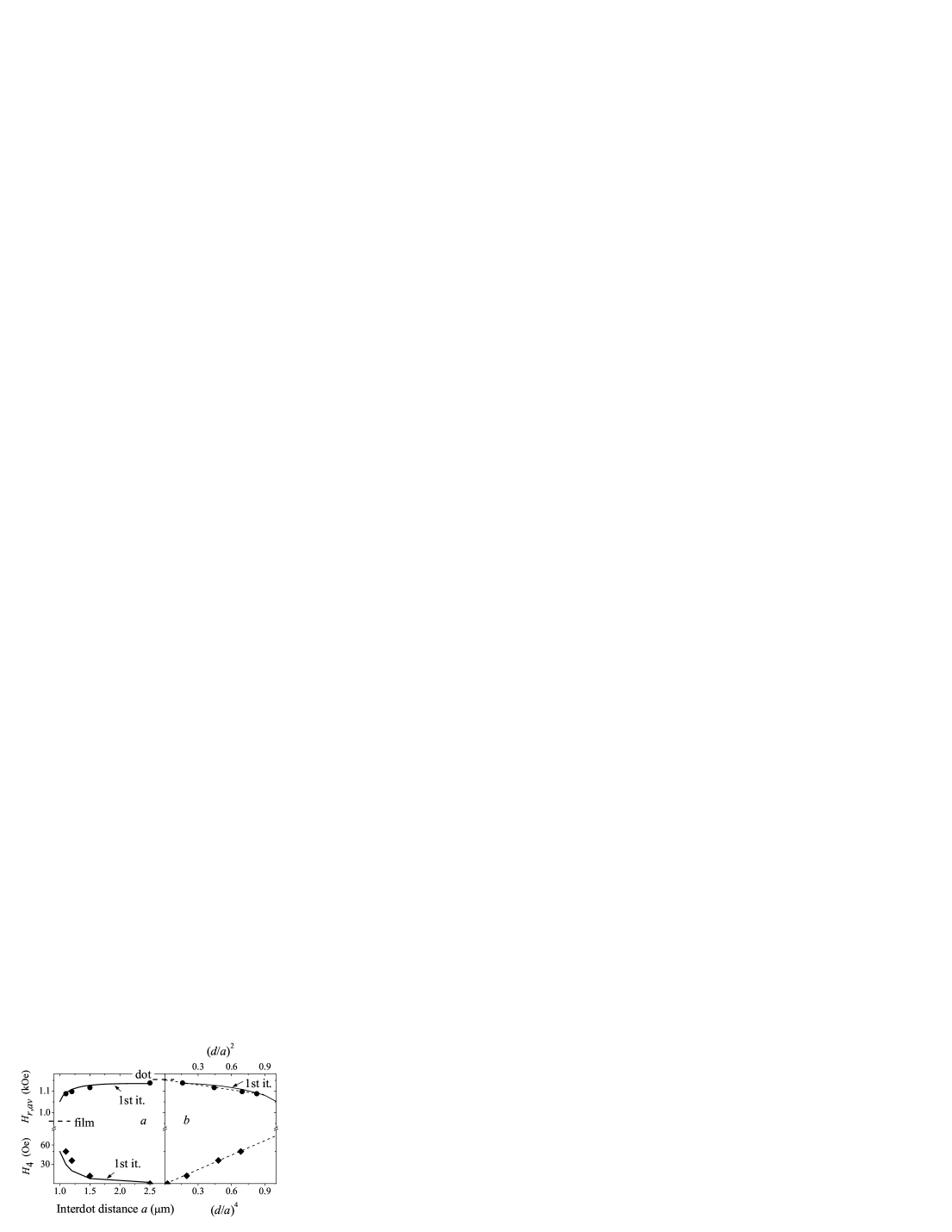
Figure 2: a) Average FMR field $H_{r,av}$ and FFA field $H_{4}$ as functions of interdot spacing $a$. The points are the experimental data and the solid lines present the 1st iteration theory (the limits mark $H_{r}$ of isolated dot and continuous film). b) The same data plotted against $(d/a)^{2}$ for $H_{r,av}$ and $(d/a)^{4}$ for $H_{4}$ give excellent linear fits (dashed lines).

The FFA effect, which could not arise in uniformly in-plane magnetized cylindrical dots, is evidently related to a non-uniform distribution of the magnetization ${\bf m}(r,\varphi,z)$ (in cylindric coordinates $0\leq r\leq R=d/2,0\leq\varphi<2\pi,0\leq z\leq t$). A similar effect was discovered using Brillouin light scattering mathieu and magnetization reversal natali ; zhu in such systems under weak enough external fields, which displace vortices in each dot. This can be modeled by displacements of two oppositely in-plane magnetized uniform domains guslienko01 . But in the presence of external fields strong enough to observe FMR, one has to assume a continuous (and mostly slight) deformation of $\mathbf{m}(r,\varphi)$. The simplest model for such deformation uses a variational procedure with respect to a single parameter metlov . However, as will be shown below, the non-uniform magnetic ground state of this coupled periodic system results from a rather complicate interplay between intra-dot and inter-dot dipolar forces, which requires a more general variational procedure.

Assuming fully planar and $z$-independent dot magnetization with the 2D Fourier amplitudes ${\bf m}_{\bf g}=\int\textrm{e}^{i{\bf g}\cdot{\bf r}}{\bf m}({\bf r})d{\bf r}$, the total (Zeeman plus dipolar) magnetic energy (per unit thickness of a dot) can be written as (see Appendix)

$$E=-\mathbf{H}\cdot{\bf m}_{0}+\frac{2\pi}{a^{2}}\sum_{{\bf g}\neq 0}\frac{f(gt)}{g^{2}}|{\bf m}_{\bf g}\cdot{\bf g}|^{2},$$ (1)

where $f(u)=1-\left(1-\textrm{e}^{-u}\right)/u$ guslienko and the vectors of the 2D reciprocal lattice are $\varphi_{H}$-dependent: ${\bf g}=(2\pi/a)(n_{1}\cos\varphi_{H}-n_{2}\sin\varphi_{H},n_{1}\sin\varphi_{H}+n_{2}\cos\varphi_{H})$ (for $\mathbf{H}\parallel x$ and integer $n_{1,2}$). The variation of exchange energy at deformations on the scale of whole sample is of the order of stiffness constant ($\sim 10^{-6}\textrm{ erg/cm}$ for Py) and it can be neglected beside the variation $\sim HM_{s}d^{2}\sim 10^{-2}\textrm{ erg/cm}$ of terms included in Eq. 1. If the dot magnetization has constant absolute value: ${\bf m}({\bf r})=M_{s}\left(\cos\varphi({\bf r}),\sin\varphi({\bf r})\right)$, its variation: $\delta{\bf m}({\bf r})=\hat{{\bf z}}\times{\bf m}({\bf r})\delta\varphi({\bf r})$ (where $\hat{{\bf z}}$ is unit vector normal to plane), is only due to the angle variation $\delta\varphi({\bf r})$. Using the Fourier transform $\delta{\bf m}_{\bf g}=\hat{\mathbf{z}}\times\sum_{{\bf g}^{\prime}}{\bf m}_{{\bf g}-{\bf g}^{\prime}}\delta\varphi_{{\bf g}^{\prime}}$ in the condition $\delta E=0$ leads to the equilibrium equation for the Fourier amplitudes:

$$m_{{\bf g},y} = \frac{4\pi}{Ha^{2}}\sum_{{\bf g}^{\prime}\neq 0}\frac{f(g^{\prime}t)}{{g^{\prime}}^{2}}({\bf m}_{{\bf g}^{\prime}}\cdot{\bf g}^{\prime})$$ (2)

$$\qquad\qquad\qquad({\bf m}_{{\bf g}-{\bf g}^{\prime}}\times{\bf g}^{\prime})\cdot\hat{{\bf z}}.$$

It can be suitably solved by iterations:

$$m^{(n)}_{{\bf g},y} = \frac{4\pi}{Ha^{2}}\sum_{\mathbf{g}^{\prime}\neq 0}\frac{f(g^{\prime}t)}{{g^{\prime}}^{2}}({\bf m}^{(n-1)}_{{\bf g}^{\prime}}\cdot{\bf g}^{\prime})$$ (3)

$$\,\qquad\qquad({\bf m}^{(n-1)}_{{\bf g}-{\bf g}^{\prime}}\times{\bf g}^{\prime})\cdot\hat{{\bf z}},$$

starting from uniformly magnetized dots as zeroth iteration: $m^{(0)}_{{\bf g},y}=0$, $m^{(0)}_{{\bf g},x}=2\pi RM_{s}J_{1}(gR)/g$ (with the Bessel function $J_{1}$). Already the 1st iteration (including the inverse Fourier transform):

$${m}^{(1)}_{y}({\bf r}) = -\theta(d-2r)\frac{8\pi^{2}R^{2}M^{2}_{s}}{Ha^{2}}\sum_{{\bf g}\neq 0}\frac{f(gt)g_{x}g_{y}}{g^{3}}\,$$ (4)

$$\qquad\qquad\qquad\qquad J_{1}(gR)\cos({\bf g}\cdot{\bf r}),$$

(with the Heavyside $\theta$ function) reveals the FFA behavior, due to the rotationally non-invariant product $g_{x}g_{y}$. The calculated maximum variation of $\varphi({\bf r})=\arcsin[m_{y}({\bf r})/M_{s}]$ in $\langle 10\rangle$ field geometry is $\sim 60\%$ bigger than in the $\langle 11\rangle$ geometry (Fig. 3, upper row). This expected behavior persists upon further iterations. Our analytic approach was checked, using the micromagnetic OOMMF code donahue on a 9$\times$9 array of considered disks (Fig. 3, lower row) at standard values of $M_{s}=0.83$ kOe and exchange stiffness $1.3\cdot 10^{-6}$ erg/cm kakazei04 for Py. The distributions obtained in this way for the central disk in the array are within $\sim 10\%$ to the analytic results of the 1st iteration.

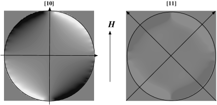
Figure 3: Density plots of the equilibrium magnetization angle $\varphi(\mathbf{r})$ for two field geometries, $\varphi_{H}=0$ ($\langle 10\rangle$) and $\varphi_{H}=\pi/4$ ($\langle 11\rangle$). Upper row: calculated from the sum, Eq. 4, over 100$\times$100 sites of reciprocal lattice at parameter values $a=1.1\,\mu$m, $H=$ 1.1 kOe, $M_{s}=$ 0.83 kOe. Lower row: micromagnetic calculation by OOMMF code for the central disc in the 9$\times$9 array.

The FMR precession of ${\bf m}({\bf r})$ is defined by the internal field $\mathbf{H}_{i}({\bf r})=\mathbf{H}+\mathbf{h}({\bf r})$ through the local dipolar field

$$h_{z}({\bf r}) = -\frac{4\pi}{a^{2}}\sum_{{\bf g}}\left[1-f(gt)\right]m_{{\bf g},z}\cos\left({\bf g}\cdot{\bf r}\right),$$

$$h_{\alpha}({\bf r}) = -\frac{4\pi}{a^{2}}\sum_{\beta,{\bf g}\neq 0}\frac{f(gt)g_{\alpha}g_{\beta}}{g^{2}}\tilde{m}_{{\bf g},\beta}\cos\left({\bf g}\cdot{\bf r}\right),$$ (5)

($\alpha,\beta=x,y$). The 1st iteration for $\mathbf{h}({\bf r})$ corresponds to the zeroth iteration for ${\bf m}({\bf r})=(M_{s},\mu_{y},\mu_{z})$, which now includes the uniform FMR amplitudes $\mu_{y},\,\mu_{z}$. Then the local demagnetizing factors $N_{x}({\bf r})=-h_{x}({\bf r})/M_{s},\,N_{y,z}({\bf r})=-h_{y,z}({\bf r})/\mu_{y,z}$ define the local FMR field $H_{r}({\bf r})$:

$$H_{r}({\bf r}) = \sqrt{H_{0}^{2}+M_{s}^{2}[N_{z}({\bf r})-N_{y}({\bf r})]^{2}/4}$$ (6)

$$- M_{s}[N_{z}({\bf r})+N_{y}({\bf r})-2N_{x}({\bf r})]/2$$

(here $H_{0}\approx 3.3$ kOe). The average FMR field is defined by the isotropic averaged demagnetizing factors

$$\overline{N}_{x,y} = \left(\pi R^{2}\right)^{-1}\int_{r<R}N_{x,y}\left({\bf r}\right)d{\bf r}$$ (7)

$$= (8\pi^{2}/a^{2})\sum_{{\bf g}\neq 0}f(gt)J_{1}^{2}(gR)/g^{2},$$

and $\overline{N}_{z}=4\pi-2\overline{N}_{x}$. At $a\to\infty$, they tend to the single dot values joseph which are for $t/R=0.1$: $N_{x,y}^{(d)}\approx 0.776$ and $N_{z}^{(d)}\approx 11.01$. Using $N_{i}^{(d)}$ instead of $N_{i}({\bf r})$ in Eq. 6 accurately reproduces the single dot FMR limit $H_{r}^{(d)}\approx 1.15$ kOe (estimated from Fig. 2b). Otherwise, for decreasing interdot distance, $a\to d$, the 1st iteration values, Eq. 7, used in Eq. 6 well describe the tendency of $H_{r,av}(a)$ towards the continuous film limit $H_{r}^{(f)}=\sqrt{H_{0}^{2}+4\pi^{2}M_{s}^{2}}-2\pi M_{s}\approx 0.96$ kOe (Fig. 2a).

Finally, by calculating the true local FMR fields $H_{r}({\bf r})$ from Eqs. 5 and 6, the field dependent absorption is obtained as $I(H)\propto\int_{r<R}\delta(H-H_{r}({\bf r}))d{\bf r}$. Then the FMR fields, $H_{r}$ defined from maximum of $I(H)$ in two geometries, display FFA in a good agreement with the experimental data (Fig. 2). This effect is due to the fact that stronger deformation of magnetization stronger suppresses the demagnetizing effect (the differences $N_{z}-N_{x,y}$) and thus enhances $H_{r}$. Also it produces a bigger spread of local resonance fields $H_{r}({\bf r})$ and thus broadens the FMR line, again in agreement with our observations.

In conclusion, it is shown that under in-plane magnetic fields, $\mathbf{H}$, even strong enough for FMR, the dipolar coupling in a dense lattice of circular magnetic dots is able to produce a continuous deformation of the dot magnetization, strongest for the field orientation along lattice axes.

Work at ANL was supported by the U.S. Department of Energy, BES Materials Sciences under Contract No. W-31-109-ENG-38; MDC was supported by FCT (Portugal) and the European Union, through POCTI (QCA III) grant No. SFRH/BD/7003/2001.

I Appendix

For fully planar and z-independent dot magnetization, the dipolar energy per unit thickness of a dot in the lattice is:

$$E_{d} = \frac{1}{2t}\int_{-t/2}^{t/2}dz\int_{-t/2}^{t/2}dz^{\prime}\int_{c}d{\bf r}\int d{\bf r}^{\prime}\sum_{\alpha,\beta}m_{\alpha}({\bf r})$$

$$\times \frac{\partial^{2}}{\partial r_{\alpha}\partial r_{\beta}}\frac{m_{\beta}({\bf r}^{\prime})}{\sqrt{\left|{\bf r}-{\bf r}^{\prime}\right|^{2}+\left(z-z^{\prime}\right)^{2}}},$$

where the 2D integrations $\int_{c}d{\bf r}$ and $\int d{\bf r}$ are respectively over the unit cell and over the entire plane. It can be also presented as

$$E_{d} = \frac{1}{2t}\int_{-t/2}^{t/2}dz\int_{c}d{\bf r}\sum_{\alpha}m_{\alpha}({\bf r})h_{\alpha}({\bf r},z)$$

$$= \frac{1}{4\pi ta^{2}}\int_{-t/2}^{t/2}dz\int_{-\infty}^{\infty}dq{\rm e}^{-iqz}\sum_{\alpha,{\bf g}}\tilde{m}_{\alpha,{\bf g}}\tilde{h}_{\alpha,{\bf g},q},$$

where the Fourier amplitudes of the dipolar field are:

$$h_{\alpha,{\bf g},q} = \int_{c}d{\bf r}\int_{-\infty}^{\infty}dz^{\prime}{\rm e}^{i({\bf g}\cdot{\bf r}+qz^{\prime})}h_{\alpha}({\bf r},z^{\prime})$$

$$= \int_{c}d{\bf r}\int_{-\infty}^{\infty}dz^{\prime}{\rm e}^{i({\bf g}\cdot{\bf r}+qz^{\prime})}\int d{\bf r}^{\prime}\int_{-t/2}^{t/2}dz^{\prime\prime}$$

$$\times \sum_{\beta}\frac{\partial^{2}}{\partial r_{\alpha}\partial r_{\beta}}\frac{m_{\beta}({\bf r}^{\prime})}{\sqrt{\left|{\bf r}-{\bf r}^{\prime}\right|^{2}+\left(z^{\prime}-z^{\prime\prime}\right)^{2}}}.$$

To calculate them, we express the lattice magnetization $m_{\beta}({\bf r}^{\prime})$ through its Fourier amplitudes:

$$m_{\beta}({\bf r}^{\prime})=\frac{1}{a^{2}}\sum_{{\bf g}^{\prime}}{\rm e}^{-i{\bf g}^{\prime}\cdot{\bf r}^{\prime}}m_{\beta,{\bf g}^{\prime}},$$

and then introduce the factor ${\rm e}^{i({\bf g}^{\prime}\cdot{\bf r}-qz^{\prime\prime})}$ into the integral in $d{\bf r}^{\prime}dz^{\prime}$, and the compensating factor ${\rm e}^{-i({\bf g}^{\prime}\cdot{\bf r}-qz^{\prime\prime})}$ into the integral in $d{\bf r}dz^{\prime\prime}$. Then the spatial integrations in $E_{d}$ are done accordingly to the formulas:

$$\int_{c}d{\bf r}{\rm e}^{i({\bf g}-{\bf g}^{\prime})\cdot{\bf r}}=a^{2}\delta_{{\bf g},{\bf g}^{\prime}},$$

$$\,\quad\int_{-t/2}^{t/2}dz\int_{-t/2}^{t/2}dz^{\prime\prime}{\rm e}^{iq(z^{\prime\prime}-z)}=\frac{4}{q^{2}}\sin^{2}\frac{qt}{2},$$

$$\qquad\quad\int_{-\infty}^{\infty}dz^{\prime}\int d{\bf r}^{\prime}{\rm e}^{i{\bf g}\cdot({\bf r}-{\bf r}^{\prime})+iq(z^{\prime}-z^{\prime\prime})}$$

$$\qquad\qquad\times\frac{\partial^{2}}{\partial r_{\alpha}\partial r_{\beta}}\frac{1}{{\sqrt{\left|{\bf r}-{\bf r}^{\prime}\right|^{2}+\left(z^{\prime}-z^{\prime\prime}\right)^{2}}}}$$

$$\qquad\qquad\qquad\qquad\qquad=\frac{4\pi g_{\alpha}g_{\beta}}{g^{2}+q^{2}}.$$

Finally, the momentum integration

$$\int_{-\infty}^{\infty}\frac{\sin^{2}(qt/2)}{q^{2}({g}^{2}+q^{2})}dq=\frac{\pi t}{2{g}^{2}}f(gt)$$

leads to the result included in Eq. 1.

References

(1)A. Moser, K. Takano, D.T. Margulies, M. Albrecht, Y. Sonobe,
Y. Ikeda, S. Sun, and E.E Fullerton, J. Phys. D: Applied Physics
35, R157 (2002); S. Sun, D. Weller, J. Magn. Soc. Jpn. 25,
1434 (2001).
(2)D.A. Allwood, Gang Xiong, M.D. Cooke, C.C. Faulkner,
D. Atkinson, N. Vernier, and R. P. Cowburn, Science 296,
2003 (2002).
(3)S.O. Demokritov, B. Hillebrands, and A.N. Slavin,
Phys. Rep. 348, 441 (2001).
(4)K.Yu. Guslienko and A.N. Slavin, J. Appl. Phys. 87, 6337 (2000);
J. Magn. Magn. Mat. 215, 576 (2000).
(5)C. Mathieu, C. Hartmann, M. Bauer, O. Büttner, S. Riedling,
B. Roos, S.O. Demokritov, and B. Hillebrands, Appl. Phys. Lett.
70, 2912 (1997).
(6) S. Jung, B. Watkins, L. DeLong, J.B. Ketterson, and
V. Chandrasekhar, Phys. Rev. B 66, 132401 (2002).
(7) M. Natali, A. Lebib, Y. Chen, I.L. Prejbeanu, and K. Ounadjela,
J. Appl. Phys. 91, 7041 (2002).
(8)X. Zhu, P. Grutter, V. Metlushko, and B. Ilic, Appl. Phys. Lett.
80, 4789 (2002).
(9)G.N. Kakazei, P.E. Wigen, K.Y. Guslienko, R.W. Chantrell,
N.A. Lesnik, V. Metlushko, H. Shima, K. Fukamichi, Y. Otani, and V.
Novosad, J. Appl. Phys. 93, 8418 (2003).
(10) V. Novosad, K. Yu. Guslienko, H. Shima, Y. Otani, S. G. Kim,
K. Fukamichi, N. Kikuchi, O. Kitakami, and Y. Shimada, Phys. Rev. B
65, 060402 (2002).
(13)M.J. Donahue and D.G. Porter, URL: http://math.nist.gov/oommf
(14)G.N. Kakazei, P.E. Wigen, K.Y. Guslienko, V. Novosad,
A.N. Slavin, V.O. Golub, N.A. Lesnik, and Y. Otani, Appl. Phys.
Lett. 85, 443 (2004).
(15)R.I. Joseph and E. Schlömann, J. Appl. Phys. 36, 1579 (1965).